Nonlocal asymmetric exclusion process on a ring and
conformal invariance

Abstract

We present a one-dimensional nonlocal hopping model with exclusion on a ring. The model is related to the Raise and Peel growth model. A nonnegative parameter $u$ controls the ratio of the local backwards and nonlocal forwards hopping rates. The phase diagram and consequently the values of the current, depend on $u$ and the density of particles. In the special case of half-filling and $u=1$ the system is conformal invariant and an exact value of the current for any size $L$ of the system is conjectured and checked for large lattice sizes in Monte Carlo simulations. For $u>1$ the current has a non-analytic dependence on the density when the latter approaches the half-filling value.

1 Introduction

One-dimensional lattice stochastic models have received a lot of attention during the last decades. Not only it is easier to reveal their properties through analytical and numerical methods but they also have interesting applications which include traffic [1] granular gases [2], the ribosomal motion of mRNA [3] bio-polymerization on nucleic acid templates [4] and statistics of DNA alignment [5].

The most researched model of this kind is the asymmetric exclusion process (ASEP) [6]. One takes a one-dimensional chain with $L$ sites covered with particles and vacancies and consider periodic or open boundary conditions where one has sources and sinks. Using sequential updating, one chooses one particle, if the neighboring sites are empty with a rate $u$ the particle hops to the left (anticlockwise) or with a rate 1 to the right (clockwise). The model is obviously local. The stationary state and more importantly, the dynamics of the model is mostly understood. The critical domain is in the KPZ [7] universality class with a dynamic critical exponent $z=3/2$. The mathematics of the model is very rich and is related to random matrix models (see [8] and references therein), and to the Bethe ansatz for quantum chains with non diagonal boundary conditions [10].

Among the extensions of ASEP, some consider nonlocal hopping. The model examined in [11] is an obvious generalization of ASEP, hoppings don’t take place only on empty neighboring sites but also on empty sites at a distance $k$ with a probability $P(k)\sim k^{-(1+a)}$. The dynamic critical exponent changes accordingly $z=\mbox{min}(a,3/2)$. Another generalization [12] consists in taking hoppings of two kinds: with a probability $p$ the particle hops all the way forward to the vacant site immediately behind the closest particle and with a probability $(1-p)$ on the next neighboring site, provide its empty. This model stays in the KPZ universality class. Another way to introduce nonlocality in the model is to consider hopping through avalanches. It was shown in [13] that depending on the density one can be in the KPZ universality class or in the diffusion ($z=2$) universality class.

A model much closer to the one we are going to present is the PushASEP model [14]. In this model, the particle hops locally to the left (anticlockwise) on the neighboring site, provide it is empty, with a rate $u$ and non locally to the right (clockwise) on the next vacant site. The beauty of the model is that one can do analytic calculations. When we are going to compare this model with ours, two exact results obtained for PushASEP are going to be relevant: the dynamic critical exponent is again $z=3/2$ and the current in a ring is a smooth function of $u$ and the density of particles $\rho$.

In the model we are going to describe and for which we use the acronym NASEP, like in PushASEP, a particle hops locally to the left with a rate $u$ and nonlocally to the right with a rate equal to 1. The crucial difference between the two models is the nonlocal hopping to the right. As we are going to explain, in NASEP the distance of the vacant site where the particle hops depends on the number of particles and vacancies encountered in the path. It turns out that this ”innocent” change will have dramatic consequences We are going to show that if we consider the ring geometry, one has a phase diagram depending on both $u$ and $\rho$ presenting gapless and gapped phases with different properties.

Before presenting our model, in Section 2, we would like to explain how we ”discovered” it (some not mathematical oriented readers might prefer to skip this part of the introduction and the Section 3 of the paper). It all started with the Raise and Peel model (RPM) [15, 16] of a fluctuating interface for an open system. This is a stochastic model where, in continuum time, the evolution rules are prescribed by a Hamiltonian which is a sum of generators of a Temperley-Lieb algebra (TL) where the parameter is fixed such that the generators form a semigroup. The vector space (configuration space) in which the Hamiltonian acts is given by RSOS (Dyck) paths. These paths represent the interface between a fluid deposited on a substrate and a rarefied gas. This model has two important features: firstly, the stationary state has wonderful combinatoric properties [17, 18] which make possible to make conjectures about the size dependence of several observables [19]; secondly, in the finite-size scaling limit, the spectrum of the Hamiltonian is known and is given by characters of the Virasoro algebra. This is possible since one has conformal invariance and the dynamical critical exponent $z=1$. Like in the previously discussed models, the model is local for left ”moves” and nonlocal for right ”moves”. This is the $u=1$ case discussed above. The model was also extended [15, 16] for $u\neq 1$. If $u>1$ the local hopping to the left is enhance whereas for $u<1$ the nonlocal hopping to the right is enhanced. New physics shows up at the price of losing integrability and mathematical beauty. As we will show in Section 2, this model can be mapped in a hopping model on a segment without sources or sinks and with an equal number of particles and vacancies (half-filling). In its new formulation, presented in this paper, one can naturally consider arbitrary densities.

We consider, for the first time, an extension of the RPM to the periodic boundary conditions case (see Section 2). This opens the possibility to study new physical phenomena (there are for example no currents in an open system without sources and sinks but they might exist in the periodic system). We start with the periodic Temperley-Lieb algebra (PTL) [20] at the semigroup point in which we use the link presentation. This gives us the model for $u=1$ and density of particles $\rho$ = 1/2. One obtains a stochastic model with again fascinating combinatorial properties of the probability distribution function describing the stationary state [17, 18]. The spectrum of the Hamiltonian can be obtained using the Bethe ansatz and, in the finite-size scaling limit, it can be written in terms of representations of the Virasoro algebra since the system, like the open case, is conformal invariant (see appendix B). The model generalizes naturally for any values of $u$ and for any densities of particles $\rho$. All the algebraic considerations can be found in Section 3.

In Appendix B, again for $u=1$, we give the connection between our model and the XXZ spin 1/2 quantum chain. This connection becomes relevant when we discuss the currents.

From now on, the text should be of interest to any reader. In Section 2 we explain the model for open and periodic boundary conditions for any backward-forward asymmetry $u$ and any density of particles $\rho$. The model is presented in two versions. The first one is in terms of particles and vacancies, this is the NASEP version of the model. The second version is in terms of charged particles (positive and negative), in this case in the sequential updating we don’t chose a particle like in NASEP but a bond. The last version is simpler and has a direct connection with the arguments presented in Section 3. If one makes the substitution positive particle $\rightarrow$ particle, negative particle $\rightarrow$ vacancy, the two versions of the model give identical results.

In Section 4 we discuss the half-filling case. For $u<1$ the system is gapped, for $u=1$ it is gapless and conformal invariant ($z=1$), for $u>1$ it is gapless but not conformal invariant ($z<1$ decreases continuously when $u$ increases). In the stationary state the current vanishes in the thermodynamical limit for any $u$ but its behavior, as a function of the size of the system $L$, reflects the phase diagram. For $u<1$, it vanishes exponentially. For $u=1$, we find for large values of $L$ ($L$ even) the expression

$$J(L)=v_{s}C/L,$$ (1.1)

where $v_{s}$ is the sound velocity and $C$ a universal constant which was determined. The current vanishes identically if $L$ is odd. The explanation of this phenomenon is given in Section 4 and Appendices A and B. We also present the $L$ dependence of the dispersion of the current in the stationary state and of the time dependence of the current. These results were obtained using Monte Carlo simulations. For $u>1$ the current vanishes like a power $J(L)\sim 1/L^{x}$ where the exponent $x$, like the exponent $z$, decreases when $u$ increases.

The currents for other densities are discussed in Section 5. For any values of $u$ the system is gapped and the currents finite in the thermodynamical limit. This implies that if we let the density approach the value 1/2, we have no phase transition if $u<1$, a usual phase transition if $u=1$ and possibly a new kind of phase transition if $u>1$. We find indeed that for $u<1$ and $u=1$ the current vanishes smoothly if the density approaches the value 1/2 but it has a non analytical dependence on the density if $u>1$. In order to understand the non-analytic behavior we had to use lattices up to 256000 sites in our Monte Carlo simulations.

Finally, in Section 6 we summarize the long list of unanswered questions.

2 A model for nonlocal asymmetric exclusion processes (NASEP)

We present two equivalent versions of the same model. One in terms of particles and vacancies (this is the NASEP formulation of the model), the other one in terms of charged particles. The first version has an obvious physical interpretation while the second is simpler and has a transparent connection with quantum chains. We give the rules when the hopping processes take place on a ring and in an open system.

One takes a lattice with sites $1\leq i\leq L$ and fill it with particles and vacancies (first version of the model) or with positive and negative particles (the second version of the model). We use sequential updating. The continuous time evolution of the system is given by the following rules:

a) The particles-vacancies version of the model.

1) On a given site one can have at most one particle (exclusion).

2) If on the site $i$ one has a particle and the preceding site $i-1$ is empty, with a rate $u$ the particle hops to the left, filling the site $i-1$, and with a rate 1 hops to the right to the empty site $i+k$. The site $k$ is chosen such that there are an equal number of particles and vacancies in the segment ($i,i+k$) AND the site $k+1$ is also empty. The number $k$ is the smallest number which satisfies these conditions (see Fig. 1a). If the site $k+1$ is full, the hopping to the right is forbidden and the particle hops only to the left with the rate $u$ (see Fig. 1b).

3) If on the site $i-1$ one has a particle, the particle on the site $i$ can hop only to the right to the site $k$ chosen as before. If the site $k+1$ is empty the hopping takes place with a rate equal to $2$ (Fig. 1c). If the site $k+1$ is full the rate is equal to 1 (see Fig. 1d)

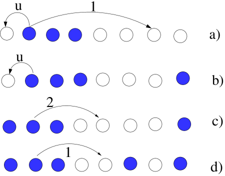
Figure 1: a,b) Hopping rules if the particle is preceded by a vacancy. c,d) Hopping rules if the particle is preceded by another particle.

The hopping to the right takes place by permuting a particle with a vacancy leaving an equal number of particles and vacancies unperturbed. The rules conserve the number of particles and can be used as such as a hopping model on a ring.

For an open system with $L$ sites, in order to apply the rules, one has to add a fictitious site $L+1$ and assume that the sites $i=1$ and $i=L+1$ are always occupied and the site $i=L$ is always empty.

Notice that in the present model, the movement to the left is local, like in ASEP, but the movement to the right is nonlocal unlike ASEP

b) The charged particles version of the model.

In this formulation of the model the sites are occupied by positive particles, which correspond to the particles in the previous formulation of the model, or by negative particles which correspond to the vacancies. The rules for the time evolution are now given considering bonds connecting two consecutive sites. A bond connecting two consecutive sites is indicated by $[c_{i-1},c^{\prime}_{i}]$, where $c$ and $c^{\prime}$ indicate the charges of the particles on the sites $i-1$, respectively $i$. The site $i$, occupied by a charge $c=\pm$, is indicated by $(c)_{i}$:

$$[(+)_{i-1},(-)_{i}]\rightarrow[(+)_{i-1},(-)_{i}]\quad{\mbox{ stays unchanged}}$$ (2.1)

$$[(-)_{i-1},(+)_{i}]\rightarrow[(+)_{i-1},(-)_{i}]\quad\mbox{rate}\quad u$$ (2.2)

$$[(+)_{i-1},(+)_{i}]+(-)_{i+k}\rightarrow[(+)_{i-1},(-)_{i}]+(+)_{i+k}\quad\mbox{rate}\quad 1$$ (2.3)

$$(+)_{i-k}+[(-)_{i-1},(-)_{i}]\rightarrow(-)_{i-k}+[(+)_{i-1},(-)_{i}]\quad\mbox{rate}\quad 1.$$ (2.4)

In (2.3) and (2.4) $k$ is chosen such that segment ($i,i+k$) and ($i-k,i-1$) contains an equal number of positive and negative particles, $k$ being the smallest number which satisfies this condition. These rules are illustrated in Fig. 2 and

Figure 2: Hopping rules for a bond connecting two charged particles.

apply to both periodic boundary conditions as well as for an open system. As one sees in Fig. 2 the hoppings take place by permuting the end particles of a neutral domain.

Let us stress that the main difference between the two versions of the model is the way the sequential updating is done in a Monte Carlo simulation. In the NASEP version one chooses randomly a particle whereas in the charged particle version, one chooses randomly a bond.

In the case of the ring geometry, by convention, if a particle (positive particle) hops from a site $i$ to a site $j$ with $j>i$, the particle moves clockwise.

In the next section we will show that if $u=1$, and one takes an equal number of particles and vacancies (equal number of positive and negative particles) and choose periodic boundary conditions the rules described above coincide with those obtained from a Hamiltonian which is a sum of generators of the periodic Temperley-Lieb algebra (TLP) [20]. In this special case, the system is conformal invariant. The present model is just an extension of the TLP case to different densities of particles and to a whole range of positive values of $u$.

For the open system, for $u=1$ and some special initial conditions, the rules can be derived from a Hamiltonian given by a sum of generators of the Temperley-Lieb (TL) algebra and the model coincides with the RPM [15, 16].

3 Representations of the Temperley-Lieb, and periodic Temperley-Lieb algebras and their connections to stochastic processes with conformal invariance

In the case of an open system, the rules described in the last section were suggested by a simple mapping of the rules of the RPM and extending them to more general cases. This model was extensively studied in the past [15, 16]. The RPM model is equivalent to the one presented in Section 2 if one has $u=1$, equal densities of particles and vacancies and certain initial conditions. In the RPM the time evolution of the system is given by a Hamiltonian which is a sum of generators of the Temperley-Lieb (TL) algebra for a special value of its parameter (see below). It is known that in this special case one can obtain exact results. The RPM was already studied away from the value $u=1$. Using a new presentation of the TL algebra described below and used in Section 2, we can study the evolution of the system for arbitrary initial conditions and densities of particles. Moreover one can give a new interpretation of the RPM using the NASEP picture instead of the interface growth interpretation used up to now. We will shortly review the open case below.

The ring geometry presented in this paper is entirely new and, as it is well known, stochastic processes on a ring have different properties than in an open system. This makes the model interesting. In order to define the model on a ring, we follow the same strategy as for the open system. This implies the following steps:

a) We consider the periodic Temperley-Lieb (TLP) algebra at the special point where it becomes a semigroup (the generators have the semigroup property, see below). The properly defined Hamiltonian written in terms of the generators of the TLP algebra defines a stochastic process in the vector space of monomials of the generators.

b) We use the spin representation of the algebra. In this representation the Hamiltonian is given by an XXZ quantum chain with an anisotropy parameter $\Delta=-1/2$ The chain has periodic boundary conditions if the number of sites $L$ is odd or has twisted boundary conditions (twist angle $\phi=-2\pi/3$) if $L$ is even [19]. These quantum chains are integrable and their spectra are known in the finite-size scaling limit, since one has conformal invariance (see appendix B).

c) We consider the link representation of the algebra which corresponds to the total spin $S^{z}=0$ ($L$ even) and $S^{z}=1/2$ or $-1/2$ ($L$ odd) sectors of the quantum chains.

d) We map the link representation to a charged particles presentation of the algebra (this is an essential step). The action of the generators in this presentation is precisely given by the rules (2.1-2.4) of Section 2 for $u=1$ and an equal number of positive and negative particles. The charged particles presentation can be mapped into a path one which is, as we are going to see, also useful.

e) We apply the same rules for arbitrary densities and introduce the parameter $u$ which favors the clockwise movements of the particles ($u<1$) or anticlockwise movements ($u>1$).

f) We map the action of the whole Hamiltonian (not of each generator) in the particles-vacancies presentation which gives the NASEP model.

We present now the whole construction of the model. The evolution operator of a system with $L$ sites is given by

$$H=\sum_{k=1}^{L-1}(1-e_{k}),$$ (3.1)

for the open system and

$$H=\sum_{k=1}^{L}(1-e_{k}),$$ (3.2)

for the periodic system. $e_{k}$ ($k=1,2,\ldots,L-1$) are the generators of the Temperley-Lieb algebra (TL), and $e_{k}$ ($k=1,2,\ldots,L$), $e_{k}=e_{k+L}$ are the generators of the periodic TL algebras at the semigroup point:

$$e_{k\pm 1}e_{k}e_{k\pm 1}=e_{k},\quad e_{k}^{2}=e_{k}\quad(k=1,2,\ldots,L-1)\quad[e_{k},e_{l}]=0\quad(|k-l|>1).$$ (3.3)

For $L$ even the periodic TL algebra has a supplementary condition which is going to be discussed below. The representation of the Hamiltonians (3.1) and (3.2) in terms of Pauli matrices are given in appendix B. We are looking for other representations of the TL algebras which give invariant subspaces (representations of ideals of the algebra). We consider first the open system.

a) The open system.

The configuration space of the TL representation we consider, has dimension $L!/(L/2+1)([L/2]!)^{2}$. Since this representation in terms of link patterns and Dyck paths, is well known we take the simple example $L=4$ to make the connection with NASEP described in Section 2. We fix the vector space (configuration space) in which the TL algebra acts. In the link representation of the TL algebra, the four sites are linked by non-intersecting arches (see Fig. 3a), the representation has dimension 2. The Dyck path representation is obtained considering the dual lattice ($\tilde{i}=0,1,\ldots,L$) and counting on each site how many times arches are crossed (Fig. 3b). It is useful to see the Dyck paths as being the border of an aggregate of tiles on top of a substrate. The right hand side of Fig. 3b is the substrate and in the left side of the picture there is one tile deposited on the substrate.

In the charged particles presentation one considers the slopes in the Dyck path. Each up (down) step corresponds to a positive (negative) particle. Notice that in both configurations one has an equal number of positive and negative particles but not all six configurations with two positive and negative particles are allowed. Only configurations in which on the left of each bond there are no more negative particles than positive ones play a role. Notice that in the model described in Section 2 all six configurations with two positive and two negative particles were considered. We will return to this point later.

In the particles-vacancies presentation, the positive particles are replaced by particles and the negative one by vacancies (Fig. 3d). The reason for using different notations for the last two vector spaces will become apparent when we will describe the action of the Hamiltonian in these vector spaces.

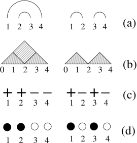
Figure 3: Different presentations of the vector space in which the generators of the Temperley-Lieb algebra acts for $L=4$ sites. a) The arch presentation, b) The Dyck path presentation, c) The charged particles presentation d) The particles-vacancies presentation.

Let us compute (see Fig. 4) the action of the generators $e_{1}$ and $e_{3}$ on the left configurations of Figs. 3a,b,c. For Fig. 4a we have used the standard action of the generators of the TL algebra on link patterns [15]. For Fig. 4b we have used the rules of the RPM [15, 16], for Fig. 4c we have used (2.3) and (2.4) with $u=1$. The same results are obtained using the mappings shown in Figs. 3a,b,c. This implies that in this configuration space, where we have desorption only (a tile is lost in the process), the dynamics of the system is given by the Hamiltonian (3.1) and the charged particles version of the model coincide.

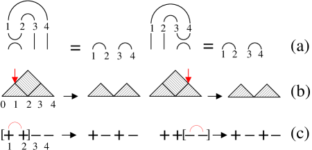
Figure 4: The action of the generators $e_{1}$ and $e_{3}$ on the configurations shown in the first column in Fig. 3. a) The arch presentation, b) The path presentation, c) the charged particle presentation. All actions take place with a rate equal to 1.

In the particle-vacancy picture (NASEP), only the particle moves, this implies that one has to consider the action of the sum of the generators $e_{1}$ and $e_{3}$ and one gets a factor of 2 (see Fig. 5 ) in agreement with the rule 3) of Section 2 (see also Fig. 1c).

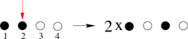
Figure 5: The hopping of the particle on the site 2 to the site 3 with a rate 2 corresponds to the action of the sum $e_{1}+e_{3}$ in Fig. 4.

What we have shown above is that for the 2 configurations in Fig. 3 the action of the Hamiltonian (3.1) which produces the desorption of a tile, coincides with the dynamics given by the rules of Section 2 (Fig. 3b).

A first generalization consists in changing the adsorption rules. This corresponds to the hopping to the left (Fig. 1a) which is equivalent to a permutation (2.2) in which a positive particle moves to the left and the negative particle to the right. This move corresponds to the action of the generator $e_{2}$ on the configuration shown in the right column of Fig .3a (see Fig. 6). The action of $e_{2}$ coincides with the rules of Section 2 (see Fig. 1a) and (2.2) only if $u=1$. If we follow the rules of Section 2 with $u\neq 1$, the evolution of the system is not anymore related to the TL algebra.

Figure 6: In the TL algebra $e_{2}$ acts with a rate $u=1$.

A second generalization of the model is obtained when we do not restrict ourselves to the two configurations of Fig. 3 by considering the 6 possible configurations with two particles and two vacancies (two positive and two negative particles respectively). Now the language of arches and Dyck paths is not useful anymore. The model describes the movement of particles in a larger vector space but one can show that the two configurations shown in Fig. 3 form an invariant subspace. This implies that if the initial conditions of the stochastic process contain only these two configurations, in the evolution of the system the remaining 4 configurations will not show up and therefore the stationary state coincides with the one obtained if one considers the two configurations only.

The discussion presented here for the 4 sites problem generalizes for any number of sites. Moreover the models discussed in Section 2 can be used for any densities of particles. We should mention that the inclusion of defects [21] in the representation of the TL algebra gives a different dynamics than the one considered in the present model since the number of particles is not conserved in this case. This closes the discussion of NASEP for an open system. In the present paper we will not discuss the properties of the open system with an enlarged space. We hope to return to this problem in the near future.

b) The periodic system.

We are going now to show that the same rules which have defined NASEP for the open system stay valid for a periodic system. For $u=1$ and half-filling they coincide with those obtained from the Hamiltonian (3.2) in which one uses the generators of the TLP algebra. The number of configurations is $L!/([L/2]!)^{2}$. We restrict ourselves again to the $L=4$ example.

Figure 7: The periodic system for $L=4$. The six configurations are shown in the arch, path, charged particles and particles-vacancies presentations.

The arch presentation of the algebra is given by oriented non intersecting arches on a puncture disc (Fig. 7) [20]. We have assigned charge particles to the sites using the following rule: if an arch starts on the site $i$ and ends on a site $j$ and does not contain the puncture, we assign a charge $(+)$ to the site $i$ and a charge $(-)$ to the site $j$. If the arch contains the puncture of the disc, we assign a charge $(-)$ to the site $i$ and a charge $(+)$ to the site $j$ (see Fig. 8). Notice that in the path picture one has the same paths as in the open case but they are now also translated because of the translational invariance on the ring. Taking into account the action of the generators on the arches (see Fig. 9b), one can check that the NASEP rules coincide with those obtained from the Hamiltonian (3.2). Notice that we have considered a quotient of the TLP algebra identifying the picture with one non contractible loop and without one. If $L$ is odd, there are no non-contractible loops since one site is attached to the puncture (see Fig. 10) and non-contractible loops are blocked by the attachment.

Figure 8: Assignment of charges to sites connected by an oriented arch which does not contain the puncture in the disc and an arch which does contain the puncture.

The charged particles presentation of the TLP algebra is as far as we know new. It is much simpler than the arch presentation. The particles-vacancies rules follow in a straightforward way. A more comprehensive discussion of the periodic Temperley-Lieb algebra is going to be presented elsewhere.

To sum up, if $u=1$ and half-filling, the NASEP model is conformal invariant since this is the case for the Hamiltonian (3.2) (see appendix B). For other values of $u$ and different densities, this is not necessarily the case. Moreover one loses integrability and all the informations about the model have to be obtained from Monte Carlo simulations.

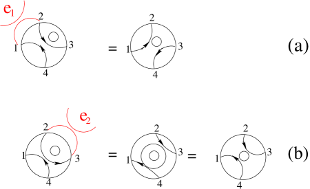
Figure 9: The action of the generators $e_{1}$ and $e_{2}$ of the periodic TLP algebra for $L=4$.

Figure 10: Loop diagram for $L$ odd, $L=5$ in this case. See the text.

We have shown that the NASEP model on a ring at $u=1$ and half-filling is conformal invariant. For $u\neq 1$ and half-filling one can assume that the phase diagram is the same as in the open system. We remind the reader what is known in this case. For $u<1$, the system is gapped, for $u=1$ it is gapless and conformal invariant (dynamic critical exponent $z=1$) and for $u>1$ it stays gapless with varying critical exponents ($z<1$ decreases if $u$ increases). A study of the correlation functions which is going to be published elsewhere [22] shows that our assumption is correct.

In the next sections we are going to study the behavior of the current in NASEP. Other features of NASEP are going to be presented in [22].

4 Currents in the NASEP model at half-filling in the stationary state

Like in ASEP, we are interested in the values of the current for various values of $u$ and densities. Unlike ASEP where the stationary state of the periodic system is trivial while the open system with sources and sinks has relevant physics, NASEP has an interesting phase diagram already for the ring geometry In this section we show that in the stationary state currents exist in NASEP at half-filling and periodic boundary conditions. We expect their behavior to be dependent on which phase of the model one is. From the study of the correlation functions [22], we have found that the phase diagram for the ring geometry coincides with the one of the open system which is the RPM. For $0<u<1$ one is in a gapped phase, for $u=1$ the system is gapless and conformal invariant and for $u>1$ it is gapless but not conformal invariant.

If the sites are denoted by $i$ ($i=1,2,\ldots,L$) with the rules of Section 2, the current is defined by the average number of particles (positive particles) which cross the bond $(i,i+1)$ moving from $i$ to $i+1$. By convention the current is positive when the particles move from $i$ towards $i+1$ and negative if they move in the other sense (anticlockwise). It is obviously independent on the bond we choose.

The existence of currents is a novel property of the model and it should be especially interesting at $u=1$. We consider this case first. We should expect on dimensional grounds and conformal invariance that, in the large $L$ limit, the current to be of the form (1.1), with the sound velocity $v_{s}=3\sqrt{3}/2$ [16] and $C$ an universal constant.

Based on numerical data on lattices up to 18, Pyatov [23] made the following conjecture for the current ($L$ even)

$$J(L)=-\frac{3L}{4(L^{2}-1)}.$$ (4.1)

From this conjecture we get the value $C$ in (1.1). The expression (4.1) was checked for large lattice sizes using Monte Carlo simulations (see Fig. 11). The existence of a current in the model was revealed because we have used the particle presentation of the model. It would have been harder to think of such a quantity in the link presentation of the TLP algebra. Of course the calculation using the NASEP version of the model gave the same result. Actually the data presented in Fig. 11 were obtained using the NASEP version of the model.

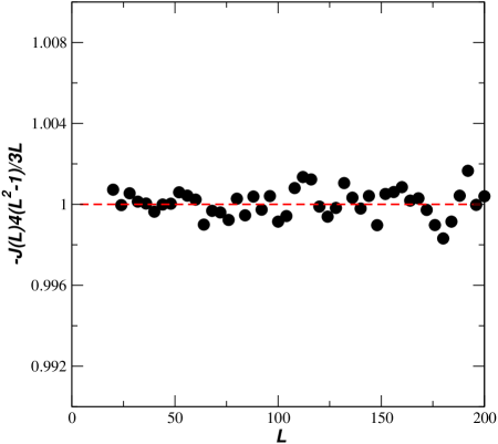
Figure 11: The current $J(L)$ divided by (4.1) for various values of $L$ at $u=1$ and half-filling. The data are obtained from Monte Carlo simulations of the NASEP model.

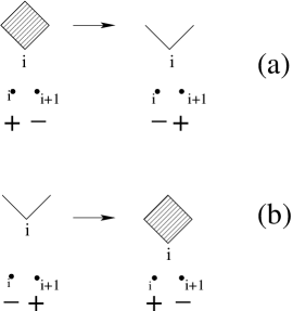
Figure 12: Contributions to the current. a) The desorption of one tile gives a +1 contribution. b) The adsorption of a tile gives a -1 contribution.

For $L$ odd one obtains $J=0$ for any size $L$. This result was obtained from small lattices and confirmed by Monte Carlo simulations.

One can understand the expression (4.1) in the following way. We start with the open system and consider the path and charged particles presentations. Notice that desorbing a tile on the site $i$ on the dual lattice gives a positive contribution to the current: a positive particle moves to the right (Fig. 12a). Similarly, adsorbing a tile on the site $i$ on the dual lattice gives a negative contribution to the current (Fig. 12b). Since in the stationary state the average number of desorbed and adsorbed tiles are the same, the average current is zero. This is what is expected for an open system.

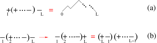
Figure 13: a) A configuration with a cluster having the size of the system. b) The effect of a tile hitting the end of the cluster (site $L$).

The situation is different if one takes periodic boundary conditions. The Dyck paths configurations are the same as in the open system but they are repeated through translations on the circle. The action of the Hamiltonian on these configurations is similar to the open case with one important exception. Let us consider a configuration with a single cluster (a Dyck path which doesn’t touch the horizontal axis except at $i=0$ and $i=L$) which has the size of the system, like in Fig. 13a. This is possible only if $L$ is even. We denote this configuration by $+(+,...,-)-$. Acting on the link $(L,1)$ (see Fig. 13b) the interchange of the two end particles produces the configuration $-(+,\ldots,-)+$ and gives one negative contribution to the current. The configuration $-(+,...,-)+$ has $L/2-1$ tiles less than the configuration $+(+,...,-)-$. These tiles didn’t give any positive contribution to the current. Since on the average the total numbers of the tiles desorbed and adsorbed are equal, one needs to have $L/2-1$ adsorbed tiles (each with a contribution -1) to compensate for the desorbed tiles. Therefore on the link $(L,1)$ one gets a total contribution to the current equal to $-1-(L/2-1)=-L/2$. On the other hand one can use a conjecture of [10] which gives the probability to have one cluster of size $L$:

$$P(L)=\frac{3L}{2(L^{2}-1)}.$$ (4.2)

Because of translational invariance there are $L$ clusters of size $L$ with a probability $3/2(L^{2}-1)$ each. Therefore the current is:

$$J(L)=\frac{3}{2(L^{2}-1)}\left(\frac{-L}{2}\right),$$ (4.3)

which coincides with (4.1). In Appendix A we discuss in detail the case $L=4$. We conclude that the appearance of the current for $L$ even comes from transitions taking place at the end of configurations having the size of the system. Such configurations, forming a single cluster, do not exist for $L$ odd (see Fig. 10), as a consequence the current should be zero. Using Monte Carlo simulations we have looked at the $L$ dependence of the current’s fluctuations in the stationary state:

$$D(L)=<J(L)^{2}>-<J(L)>^{2},$$ (4.4)

where $J(L)$ is given by (4.1) and $<J(L)^{2}>$ is the average of the square of the current for a system of size $L$. We have used lattices of size $L=$ 500, 1000, 2000, 4000, 8000, 16000, 32000 and 64000. A fit to the data gave

$$D(L)=a/L^{b}\quad{\mbox{ with }}\quad a=0.21\pm 0.04,\quad b=0.86\pm 0.03.$$ (4.5)

We are still missing an interpretation of the exponent $b$.

The time dependence of the current for different values of $L$ was also explored. We used the step initial condition (particles filling one half of the lattice and vacancies filling the other half). Using conformal invariance, we expect the following behavior of the current:

$$J(t,L)=\frac{1}{t}f(\frac{L}{t}),$$ (4.6)

where $f(L/t)\sim\frac{3}{4}t/L$ for $L/t\to 0$, and $J\sim\frac{3}{4}v_{c}1/t$ for $t/L\to 0$ ($v_{c}=3\sqrt{3}/2)$).

The data are shown in Fig. 14 in which we have plotted $t|J(t,L)|$ as a function of $L/t$. Lattices of size 300, 600 and 1200 were chosen and the time unit was chosen 100 times smaller than the usual one. One observes a nice data collapse at small values of $L/t$ and large finite-size effects for large values of $L/t$ probably due to the choice of the initial condition.

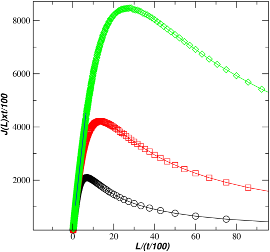
Figure 14: The current $J(t,L)$ multiplied by $t/100$ as a function of $100L/t$ for the sizes $L=300$ (in green), $L=600$ (in red) and $L=1200$ (in black).

Taking $u$ away from the value 1 is bound to change the picture. For $u<1$ one has a larger desorption (loss of tiles) and for a given lattice size $L$, one expects a decrease of the absolute value of the current, the opposite phenomenon should take place at $u>1$. At a given value of $u$, one expects the current to vanish exponentially for $u<1$ (one is in the gapped phase) and to vanish as a power of $L$ for $u>1$ (one is in a non-conformal invariant gapless phase). This is what is observed.

In Fig. 15 we show the current $J(L)$ as a function of $L$ for $u=0.75$ obtained in Monte Carlo simulations. A good fit to the data gives:

$$J(L)=-0.0036\exp(-0.0225L),$$ (4.7)

confirming the expected exponential decrease of the current with $L$ in the gapped phase.

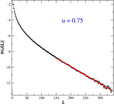
Figure 15: The current as a function of $L$ ($L$ even) for $u=0.75$. Lattices of size $4,6,8,\ldots,340$ were considered in the Monte Carlo simulations. The fitting curve is also shown.

The case $u>1$ is shown in Fig. 16 where the $u=5$ data are shown. A fit to the data gives:

$$J(L)=-0.917/L^{0.132}$$ (4.8)

In the whole phase $u>1$ the current behaves like $J\sim-1/L^{x}$. For example $x=0.182$ for $u=3$. The exponent $x$ decreases with $u$, this implies that the absolute value of the current increases with $u$. This is to be expected since large clusters have more chance to occur for large values of $u$, and hence more clusters having the size of the system.

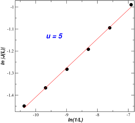
Figure 16: The current as a function of $L$ ($L$ even) for $u=5$ and half-filling, obtained from Monte Carlo simulations, for lattice sizes $L$=1000, 2000, 4000, 8000, 16000 and 32000. The fitting line is also shown.

Up to now we have considered the case of $L$ even only and mentioned that for $u=1$ the current vanishes for all values of $L$ odd, this is not the case for other values of $u$. We present now in more detail the data which show the $u$ dependence of the current for even and odd lattices. In Fig. 17 we compare the behavior of the currents for $L$ even and odd, for small lattice sizes, for which one can obtain numerically exact results.

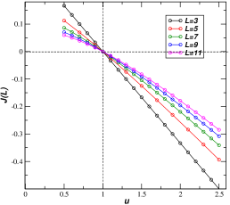
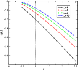
Figure 17: Exact values of the current for small lattice sizes at half-filling: a) even number of sites, b) odd number of sites.

For $L$ even, one notices that the current stays negative for all values of $u$, its absolute value increasing with $u$. For $L$ odd the situation is different. For $u<1$ the current is positive, vanishes for $u=1$ and changes in sign for $u>1$. For large lattices and $u>1$, the ratios of the currents even/odd are close to 1. For example for $u=5$ and $L=32000$ we obtain: $J(L)/J(L+1)=1.06$.

To sum up, for half-filling in the thermodynamical limit the current vanishes for all values of $u$. This picture is going to change dramatically away from half-filling.

5 Currents at other densities.

As we have seen at half-filling, in the thermodynamical limit, the currents vanish for any value of $u$. This picture changes if the density of particles (positive particles) $\rho$ is not equal to 1/2. It is convenient to look at the deficit of density of particles $\eta=1/2-\rho$.

We start by observing that for any $\eta\neq 0$ and any $u$ the system is gapped. This information comes from the study of correlation functions which have all an exponential decay [22].

At $u=1$, from an exact analysis of small lattice sizes and from Monte Carlo simulations on large lattices sizes, one can conclude that for any value of $\eta\neq 0$, the currents vanish for large lattice size $L$. For other values of $u$, the current stays finite. This property is illustrated in Fig. 18 where the currents are given for the three values $\eta=1/42$, 1/6 and 1/4 and different lattice sizes. One notices that for a given value of $\eta$ one has data collapse of several lattice sizes. The current is negative for $u>1$ and positive for $u<1$.

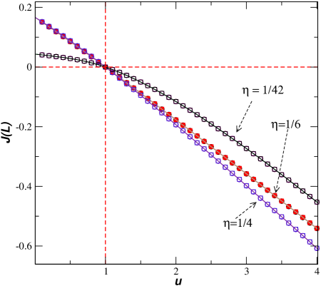
Figure 18: The currents $J(L)$ as a function of $u$ for $\eta=1/42,1/6$ and $1/4$, and $L=1000,2000,4000,8000,16000$ and 32000.

The currents approach their asymptotic values with a correction term $\sim 1/L$. This is illustrated in Fig. 19, where we have taken $\eta=1/4$ and $u=5$. A fit to the data gives $J(L)=-0.72-0.82/L$. The same occurs for $u<1$. For example taking $u=0.75$ and $\eta=1/4$ one gets $J(L)=0.04+0.05/L$.

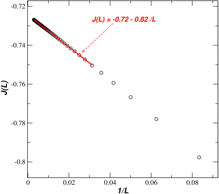
Figure 19: The current $J(L)$ as a function of $L$ for $u=5$ and $\eta=1/4$, $L=16,20,24,...,340$. The fitted curve is also shown.

The most interesting feature of the current behavior occurs if, for fixed $u$, one looks at its variation with $\eta$. A first impression about the $\eta$ dependence of the current can be obtained from the data for several values of $u$, shown in Fig. 20, where we considered the small lattice size $L=30$. We observe that, as expected, the currents are symmetric functions of $\eta$, and that they are positive for $u<1$ and negative for $u>1$. We also see for larger values of $u$, a kind of plateau around $\eta$ = 0. This observation is a precursor of a phenomenon seen for large lattices.

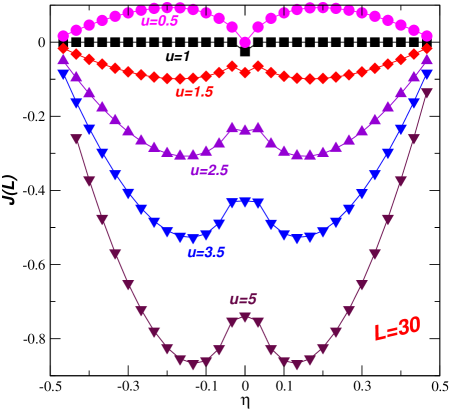
Figure 20: The current $J(30)$ as a function of $\eta$ for several values of $u$.

We start by looking the data for fixed $u=0.75$ ($u<1$). They are shown in Fig. 21.

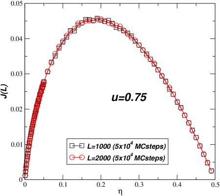
Figure 21: The current $J(L)$ for $u=0.75$ as a function of $\eta$ for lattice sizes $L=1000$ and 2000.

This is the expected behavior since the current has to vanish at $\eta=0$ and 0.5 (there are no particles to carry the current in this latter case). Similar results are obtained for other values of $u<1$.

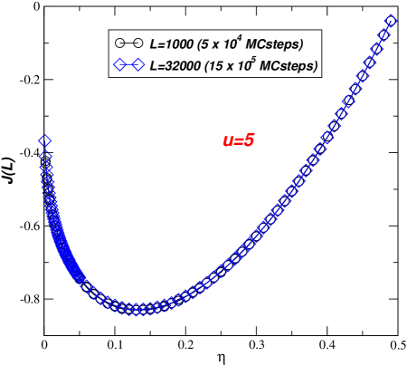
Figure 22: The current $J(L)$ for $u=5$ as a function of $\eta$. The data are from lattice sizes $L=1000$ and 32000.

The situation is dramatically different if $u>1$. In Fig. 22 we show the data for $u=5$. One notices that if $\eta$ approaches the zero value (almost half-filling) the current stays finite. It has the value -0.37 for $\eta=0.001$ for a lattice of size $L=32000$. As we have discussed, the current vanishes at $\eta=0$ and this implies a phase transition of a new kind since the current has a discontinuity. The discontinuity increases with $u$ (it vanishes at $u\leq 1$). This is illustrated in Fig. 23 where we show, as a function of $u$, the values of $J(L)$ for $\eta=0.001$ and three lattice sizes.

The appearance of this phase transition came as a surprise. We have tried to understand its origin by looking at another quantity which is relevant to the existence of the current: the density of vacancy-particle pairs $\rho_{v-p}$ (negative positive particles pairs or valleys in the language of Dyck paths) in the stationary states. In the case $\eta=0$, this quantity was already studied for various values of $u$ for the open system and we don’t expect big changes for the periodic system. This is at least the situation for $u=1$ for which this density is equal to $\rho_{v-p}=3/8=0.375$ for the open and periodic systems[19]. We expect this quantity to decrease for larger values of $u$ [16].

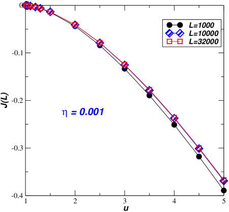
Figure 23: Illustration of the discontinuity of the current for $\eta\neq 0$. The current as a function of $u$ for $\eta=0.001$ for the lattice sizes $L$=1000, 10000 and 32000.

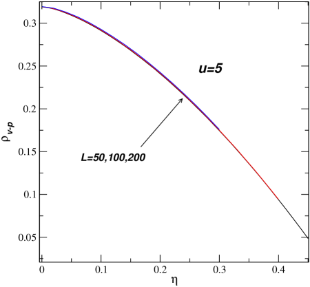
Figure 24: The density of vacancy-particle pairs as a function of $\eta$ for $u=5$ and lattice sizes $L=50,100$ and 200.

In Fig. 24 we show for $u=5$ the density of pairs $\rho_{v-p}$ as a function of $\eta$ for three lattice sizes. One clearly sees data collapse already for relatively small lattice sizes, and no discontinuity is observed. Moreover the value 0.31, at the density at $\eta$ = 0 is compatible with the known result [16] for the open system. This observation made us think that may be the phase transition is a red herring.

If we do have a novel phase transition we expect the current to have the following behavior at finite $L$:

$$J(L)=A\eta^{x},$$ (5.1)

with the exponent $x$ decreasing with $L$ such that in the thermodynamic limit, $x=0$. If on the other hand we don’t have the novel phase transition, one can explain the data by having just very small values of the exponent $x$ which fake the phase transition. If this is the case, $x$ could even slightly increase with $L$. Taking into account that in Figs. 21 and 22 we have used lattices up to 32000 sites and went to densities very closed to the half-filling value ($\eta=0.001$), in order to clarify the issue, we decided to consider lattices up to 256,000 sites and values of $\eta$ as small as $0.000005$. In order to interpret the data we have to keep in mind that we are in a gapped phase and, consequently, at a fixed value of $\eta$ the data should converge exponentially for large values of $L$.

In Fig. 25 for $u=3$, we show the current as a function of $\eta$ for several lattice sizes between 500 and 256,000. One notices that for very small fixed values of $\eta$ the absolute value of the current keeps slightly decreasing even for very large lattices. The existence of the novel phase transition, would have implied an $L$ independent constant value of the current.

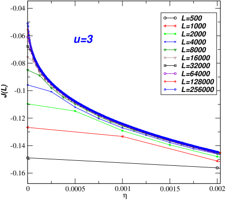
Figure 25: The current as a function of $\eta$ for $u=3$. Lattices with sizes increasing by a factor of 2 from 500 to 256.000 were considered.

The situation becomes even clearer if we examine the data shown in the next figure (Fig. 26) where the results for the largest lattices ($L=128,000$ and $L=256,000$) are presented only. The results of the fits using (5.1) are very interesting. One obtains:

$$A=0.333,\quad x=0.152,\quad L=128,000\quad(\mbox{region 1}),$$

$$A=0.338,\quad x=0.156,\quad L=256,000\quad(\mbox{region 1}),$$

$$A=0.293,\quad x=0.142,\quad L=256,000\quad(\mbox{region 2}).$$

The region 1 contains ”larger” values of $\eta$, Region 2 ”smaller” values. Within errors, the values of $x$ for the two regions coincide and are not equal to zero. The difference between the values of $x$ for the two Regions is minimal. A good fit for all the data gives $A=-0.30\pm 0.05$, $x=0.145\pm 0.005$. We conclude that there is no novel phase transition. The current vanishes smoothly albeit in a non-analytic way when $\eta$ vanishes. This could have been expected since we have a transition from a gapped phase to a gapless one but it was a long way to get to this conclusion.

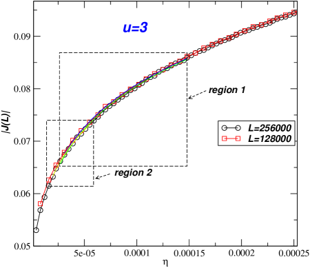
Figure 26: The very small $\eta$ domain. The absolute value of the current as a function of $\eta$ for $L=128,000$ and 256,000.

The existence of a non-analytic behavior of the current, but albeit no phase transition of a new kind, was seen for various values of $u$. The exponent $x$ and the factor $A$ are given for several values of $u$ in table 1. It looks like $x$ increases to the value one if $u$ approaches the value 1. This is a reasonable guess since $x=1$ for $u<1$ (we have no phase transition in this domain and we expect an analytic dependence on $\eta$). In order to confirm the value $x=1$ for $u<1$, we have included several values of $u<1$ in table 1. For all these values of $\eta$ one finds $x\approx 1$ indeed.

$u$ $A$ $x$ 0.0625 $1.90\pm 0.01$ 1 (*) 0.125 $1.85\pm 0.01$ 1 (*) 0.25 $1.70\pm 0.01$ 1 (*) 0.5 $1.40\pm 0.05$ $0.994\pm 0.005$ 0.75 $1.13\pm 0.05$ $0.99\pm 0.01$ 1 0.0 - 1.25 $-0.043\pm 0.001$ $0.343\pm 0.005$ 1.5 $-0.060\pm 0.001$ $0.245\pm 0.002$ 1.75 $-0.089\pm 0.001$ $0.205\pm 0.005$ 2 $-0.130\pm 0.005$ $0.180\pm 0.005$ 3 $-0.30\pm 0.05$ $0.145\pm 0.005$ 4 $-0.48\pm 0.02$ $0.12\pm 0.01$ 5 $-0.70\pm 0.05$ $0.110\pm 0.005$ 7 $-1.15\pm 0.05$ $0.085\pm 0.05$ 10 $-1.75\pm 0.05$ $0.065\pm 0.05$

Table 1: Values of the parameters $A$ and $x$ in the behaviour (5.1) of the density of current $J$ as a function of the density $\eta$, for several values of $u$. These estimates were obtained by considering values of $\eta<0.00025$ and lattice sizes $L=128K$ and $L=256K$ for the periodic RPM model. The lines with (*) are obtained by a linear fit, since in this case the fit is much better.

6 Conclusions

In this paper the Raise and Peel model is reformulated as a nonlocal asymmetric exclusion process (NASEP). We extend and study the model in the case of periodic boundary conditions and arbitrary densities of particles. NASEP depends on two parameters $u$ and the density of particles $\rho$. The parameter $u$ gives the forward-backward asymmetry of the model.

At half-filling and $u=1$, the system is conformal invariant (dynamic critical exponent $z=1$) and the spectrum is known in the finite-size scaling limit [9]. The system is integrable (see Appendix B) and the probability distribution function describing the stationary state has remakable combinatorial properties [17, 18]. Still at half-filling, if $u<1$, the system is gapped while for $u>1$, the system is gapless with the critical exponent $z$ varying continuously with $u$ ($z(u)<1$). The function $z(u)$ decreases with $u$. At any density $\rho\neq 1/2$ the system is gapped. This implies that getting $\rho$ closed to the value 1/2, we have no phase transition if $u<1$, a usual phase transition if $u=1$ and possibly a new kind of phase transition if $u>1$.

We have studied the current in NASEP. This was possible because of the extension of the model to periodic boundary conditions. In stationary (nonequilibrium) states the current can be seen as an order parameter and its properties should reflect the phase diagram. This is indeed the case. At half-filling and even lattice size $L$, the current vanishes exponentially for $u<1$, and as $L^{-x(u)}$ otherwise ($x(u)<1$). If $u=1$ it has the expression (1.1) with $C$ an universal constant. This implies that at half-filling the current vanishes in the thermodynamic limit for any $u$. For $L$ odd the current vanishes identically for any $L$ and $u$. If we are not at half-filling, the current stays finite in the thermodynamic limit for any density and asymmetry $u$.

It is interesting to see how the current vanishes as a function of $\eta=\rho-1/2$ when $\eta$ approaches the value zero. For $u<1$, the current vanishes linearly with $\eta$, for $u=1$ it vanishes for any number of sites. For $u>1$ it vanishes like $\eta^{x}$ where the exponent $x$ decreases with $u$, getting very small values for moderate values of $u$. Finding the exponent $x$ using Monte Carlo simulations (see table 1) was not an easy task. One had to use very large lattices (up to 256,000 sites).

This paper is going to be followed by a sequel [22] in which we present the fluctuations of the current and various correlation functions.

In Section 3 we derive the model for $u=1$ and half-filling using the periodic Temperley-Lieb algebra. In Appendix B we make the connection of the model with integrable quantum chains and derive the expression of the spin current. The fact that the spin current vanishes for any size $L$ ($L$ odd) is also shown. Notice that the spin current has a behavior similar to the NASEP current.

The reader might have noticed that the expression Bethe ansatz was not used in the text except in Appendix B. This is not an accident. Unlike in TASEP or PushASEP where a lot of work was done (see [24, 25, 26, 27] and references therein), up to now a whole class of questions were not asked yet in the case of NASEP. For example, we didn’t look at large time fluctuations of observables by starting with flat or step initial conditions [14, 28] and checked for the existence of an equivalent of so-called Airy processes. Since for $u=1$ and half-filling the system is integrable one might hope that some pretty properties might show up.

We have to mention that for an open system the description of NASEP can be found in Section 2. The formulation of the model in the presence of sources and sinks at the boundaries remains to be done. Finally, a very relevant question about out work stays still without an answer: we keep looking for physical applications.

7 Acknowledgments

VR would like to thank DFG (project RI 31716-1) and FCA to FAPESP and CNPq (brazilian agencies) for financial support. We also thank V. Priezzhev for very fruitful discussions.

Appendix A Appendix: The current for four and three particles on a ring for $u=1$

We present first the calculation of the current on a ring in the case of two $(+)$ and two $(-)$ ($L$ even) particles and next the case of two $(+)$ and one $(-)$ particles ($L$ odd). This calculation will make clear why one has a current in the first case and not in the second.

There are 6 configurations for $L=4$ shown in Fig. 7. We consider the configuration $++--$ on the sites 1,2,3 and 4. In this configuration one has a tile on top of the substrate. We apply the rules of Section 2 (see (2.1)-(2.4)) on each of the four bonds in order to find out which configurations one obtains. We keep track on the number of tiles lost or won and of the current on the bond. We repeat the same procedure also for the configuration $+-+-$ on the ordered 4 sites. No tiles are present in this case. The results are shown in table 2 where we denote by $[\ \ ,\ \ ]$ a bond.

$|{\mbox{in}}>\rightarrow|{\mbox{out}}>$ Tiles Current $[+_{1}+_{2}]-_{3}-_{4}\rightarrow+_{1}-_{2}+_{3}-_{4}$ -1 +1 $+_{1}+_{2}[-_{3}-_{4}]\rightarrow+_{1}-_{2}+_{3}-_{4}$ -1 +1 $+_{4}]+_{1}-_{2}[-_{3}\rightarrow+_{4}-_{1}+_{2}-_{3}$ -1 -1 !!! $+_{1}[+_{2}-_{3}]-_{4}\rightarrow+_{1}+_{2}-_{3}-_{4}$ 0 0 $[+_{1}-_{2}]+_{3}-_{4}\rightarrow+_{1}-_{2}+_{3}-_{4}$ 0 0 $+_{1}-_{2}[+_{3}-_{4}]\rightarrow+_{1}-_{2}+_{3}-_{4}$ 0 0 $+_{1}[-_{2}+_{3}]-_{4}\rightarrow+_{1}+_{2}-_{3}-_{4}$ +1 -1 $+_{1}]-_{2}+_{3}[-_{4}\rightarrow+_{1}+_{2}-_{3}-_{4}$ +1 -1

Table 2: The dynamics of 4 sites. The other processes not shown are obtained by cyclic permutation of the presented ones.

The results for other configurations are obtained by simple permutations. One can diagonalize the Hamiltonian obtained from table 2 and find that in the stationary state each of the four configurations with two adjacent (+) charges have the probability 1/10 and each of the two configurations with no tiles have a probability 3/10.

Let us first note that in the stationary state (see table 2), the average number of tiles desorbed equal to $3\times 4\times 1/10$ is equal to the number of tiles adsorbed $2\times 2\times 3/10$. With one exception, each desorbed tile contributes one positive unit to the current while each adsorbed tile gives a negative unit. If one wouldn’t have an exception, the current would have been zero like in the open system. The exception occurs when one considers the bond $[-\;+]$ on the sites $[4,1]$. Although one looses a tile one gets a negative contribution to the current. This phenomena is the origin of a negative current. A simple arithmetic gives a current equal to -1/5. There is another simpler derivation of the value of the current. If on the bond $[4,1]$ one would have had a (+1) contribution to the current, the total current would be equal to zero (like the balance of the number of tiles). One has therefore subtract and add this value to obtain a net contribution of -2 to the current. Since the probability of the configuration is 1/10, one recovers the value -1/5 in agreement with (4.2).

This simple way of reasoning does not apply for an odd number of sites. Let us consider the case $L=3$ on a ring as an example. One has 3 configurations with a probability 1/3 each: $++-$, $+-+$ and $-++$. For an open system one has 2 of them in the relevant subspace: $++-$ and $+-+$ and one can attribute a tile to the first configuration and none to the second. One can then show that the average number of tiles in the stationary state is 1/2. In the periodic system the 3 configurations can be seen as having all one tile or none. Applying the rules (2.1) one can show that the current vanishes.

Appendix B Appendix: The spin current in the spin presentation of the periodic Temperley-Lieb algebra

The time evolution in NASEP is given by a non-hermitian Hamiltonian. We are going to show that his Hamiltonian also acts taking a different basis, in a sector of a hermitian Hamiltonian that we are going to derive. The new Hamiltonian describes an integrable quantum spin chain about which a lot is known. We will compute the spin current in this chain and compare it with the current derived in Section 4. We have to stress that all results presented in this Appendix are related to the case $u=1$ and half-filling of NASEP.

The TLP algebra at the semigroup point is defined in Eq. (3.3). For $L$ odd, the generators have the following presentation in terms of Pauli matrices [19]:

$$e_{i}=\sigma_{i}^{+}\sigma_{i+1}^{-}+\sigma_{i}^{-}\sigma_{i+1}^{+}-\frac{1}{4}\sigma_{i}^{z}\sigma_{i+1}^{z}-i\frac{\sqrt{3}}{4}(\sigma_{i}^{z}-\sigma_{i+1}^{z})+\frac{1}{4},$$ (B.1)

where $i=1,2,...L$, and $e_{L+1}=e_{1}$. Using (3.2) one obtains the Hamiltonian in the spin representation:

$$H=-\sum_{i=1}^{L}\left[\sigma_{i}^{+}\sigma_{i+1}^{-}+\sigma_{i}^{-}\sigma_{i+1}^{+}-\frac{1}{4}\sigma_{i}^{z}\sigma_{i+1}^{z}-\frac{3}{4}\right],\quad\mbox{($L$ odd)}.$$ (B.2)

This is a hermitian periodic Hamiltonian. The picture is different if $L$ is even. The first $L-1$ generators have the expression (B.1) but $e_{L}$ is different:

$$e_{L}=\sigma_{L}^{+}\sigma_{1}^{-}e^{i\phi}+\sigma_{L}^{-}\sigma_{1}^{+}e^{-i\phi}-\frac{1}{4}\sigma_{L}^{z}\sigma_{1}^{z}-i\frac{\sqrt{3}}{4}(\sigma_{L}^{z}-\sigma_{1}^{z})+\frac{1}{4},$$ (B.3)

where $\phi=-2\pi/3$. Using (3.2) one obtains the Hamiltonian:

$$H = -\sum_{i=1}^{L-1}\left[\sigma_{i}^{+}\sigma_{i+1}^{-}+\sigma_{i}^{-}\sigma_{i+1}^{+}+\frac{1}{4}\sigma_{i}^{z}\sigma_{i+1}^{z}-\frac{3}{4}\right]$$ (B.4)

$$-\sigma_{L}^{+}\sigma_{1}^{-}e^{i\phi}-\sigma_{L}^{-}\sigma_{1}^{+}e^{-i\phi}+\frac{1}{4}\sigma_{L}^{z}\sigma_{1}^{z}+\frac{3}{4},\quad\mbox{($L$ even)}.$$

This is an hermitian Hamiltonian with twisted boundary condition: $\sigma_{L+1}^{\pm}=\exp(\mp i\phi)\sigma_{1}^{\pm}$, characterized by the twist angle $\phi$. It is known that the two Hamiltonians (B.2) and (B.4) are integrable and their finite-size scaling spectra are known [30]. The operator

$$S^{z}=\sum_{i=1}^{L}\sigma_{i}^{z}$$ (B.5)

commutes with the Hamiltonians and for half-filling ($L$ even) the spectrum of NASEP coincides with the spectrum of the Hamiltonian (B.4) in the sector $S^{z}=0$. For $L$ odd NASEP is in the $S^{z}=1/2$ (or equivalently $-1/2$) sector. The basis of positive and negative particles (particles and vacancies) is however different from the spin up $\leftrightarrow$ down spin basis of Pauli matrices. There is a similarity transformation which relates the two basis. Following [29] we are going to compute the spin currents for the $L$ odd and even and compare the obtained currents with those of NASEP. To do so, using a similarity transformation we bring the Hamiltonian (B.4) to the form:

$$H=-\sum_{i=1}^{L}\left[\sigma_{i}^{+}\sigma_{i+1}^{-}e^{i\frac{\phi}{L}}+\sigma_{i}^{-}\sigma_{i+1}^{+}e^{-i\frac{\phi}{L}}-\frac{1}{4}\sigma_{i}^{z}\sigma_{i+1}^{z}-\frac{3}{4}\right]\quad(L{\mbox{ even}}).$$ (B.6)

The spin current operator on the bond $[i,i+1]$ is

$$J_{i}^{z}=i(\sigma_{i}^{+}\sigma_{i+1}^{-}-\sigma_{i}^{-}\sigma_{i+1}^{+}).$$ (B.7)

If $E(\phi,L)$ is the ground-state energy for system of size $L$ and twist angle $\phi$. Using (B.6), (B.7) and translational invariance, one obtains in leading order in $L$ the following expression for the average value of the spin current:

$$J^{z}=\langle 0|J_{i}^{z}|0\rangle=-\frac{\partial E(\phi,L)}{\partial\phi}.$$ (B.8)

Since for $L$ odd there is no twist (one has periodic boundary conditions), it follows that the current vanishes, like in NASEP. For $L$ even one can use the results of Ref. [31] (Eq. (3.25)):

$$\frac{\partial E(\phi,L)}{\partial\phi}=\frac{3v_{s}\phi}{4\pi L},$$ (B.9)

where $v_{s}=3\sqrt{3}/2$ is the sound velocity. Taking into account that $\phi=-2\pi/3$ one obtains finally

$$J^{z}=-\frac{3\sqrt{3}}{4L},$$ (B.10)

which, up to a factor $\sqrt{3}$, coincides with NASEP current (4.4) for large values of $L$. Notice that we did a quantum mechanical calculation in an equilibrium state and did not consider the stationary state of a stochastic process.

References

- [1] Nagel K and Schreckenberg M, 1992 J. de Physique I 2 2221
- [2] Torok J, 2005 Physica A 355 374
- [3] Shaw L B, Zia R K P and Lee K H P, 2003 Phys. Rev. E 68 0219010
- [4] Parmeggiani A, Franosch T, and Frey E, 2003 Phys. Rev. Lett. 90 086601
- [5] Berg O G, Winter R B, and von Hippel P H, 1981 Biochemistry 20, 6929
- [6] Derrida B, Domany E and Mukamel D, 1992 J. Stat. Phys. 69 667; Derrida B, Evans M R, Hakim V and Pasquier V, 1993 J. Phys. A bf 26 1493
- [7] Kardar M, Parisi G, and Zhang Yi-C, 1986 Phys. Rev. Let. 56 889
- [8] Ferrari P L ,2010 J. Stat. Mech P10016
- [9] de Gier J and Essler F H L, 2006 J. Stat. Mech. P12011
- [10] de Gier J, 2005 Discr. Math. 298 365
- [11] Szavits-Nossan J and Uzelac K, 2008 Phys. Rev. E 77 051116
- [12] Ha M, Park H and den Nijs M, 2007 Phys. Rev. E 75 061131
- [13] Priezzhev V B, Ivashkevich E V, Povolotsky A M, and Hu C -K, 2001 Phys. Rev. Lett. 8 084301
- [14] Borodin A, Ferrari P L, 2008 J. Probab. 13 1380
- [15] de Gier J, Nienhuis B, Pearce P A, and Rittenberg V, 2004 J. Stat. Phys. 114 1
- [16] Alcaraz F C and Rittenberg V, 2007 J. Stat. Mech. P07009
- [17] Razumov A V and Stroganov Yu G, 2005 Theor. Math. Phys. 142 237; 2005 [Teor. Mat. Fiz. 142 284]
- [18] Cantini L and Sportiello A, 2011 Journ. of Comb. Theory A118 1549
- [19] Mitra S, Nienhuis B, de Gier J and Batchelor M T, 2004 J. Stat. Mech. P09010
- [20] Martin P and Saleur H, 1993 Comm. Math. Phys. 158 155
- [21] Pearce P A, Rasmussen J, and Villani S P, 2010 J. Stat. Mech. P02010
- [22] Alcaraz F C and Rittenberg V, to be published
- [23] Pyatov P, private communication
- [24] Ferrari P L, Frings R, 2011 J. Stat. Phys. 144 1123
- [25] Prolhac S and Spohn H, 2011 J. Stat. Mech. P01031
- [26] Corwin I, 2011 arXiv:1106.1596
- [27] Thomas Gueudre T, Pierre Le Doussal P, Alberto Rosso A, Adrien Henry A, Pasquale Calabrese P, 2012 Phys. Rev. E 86 041151
- [28] Borodin A, Ferrari P L and Sasamoto T, 2008 Comm. Math. Phys. 283 417
- [29] Shastry B S and Sutherland B, 1990 Phys. Rev.Lett. 65 243
- [30] Alcaraz F C, Baake M, Grimm U and Rittenberg V, 1988 J. Phys. A 21 L117
- [31] Alcaraz F C, Barber M N and Batchelor M T, 1988 Ann. Phys. 182 280