Quantum information-geometry of dissipative quantum phase transitions

Abstract

A general framework for analyzing the recently discovered phase transitions in the steady state of dissipation-driven open quantum systems is still missing. In order to fill this gap we extend the so-called fidelity approach to quantum phase transitions to open systems whose steady state is a Gaussian Fermionic state. We endow the manifold of correlations matrices of steady-states with a metric tensor $g$ measuring the distinguishability distance between solutions corresponding to different set of control parameters. The phase diagram can be then mapped out in terms of the scaling-behavior of $g$ and connections with the Liouvillean gap and the model correlation functions unveiled. We argue that the fidelity approach, thanks to its differential-geometric and information-theoretic nature, provides novel insights on dissipative quantum critical phenomena as well as a general and powerful strategy to explore them.

Introduction:–  The occurrence of typical equilibrium phenomena in out equilibrium driven condensed matter systems (e.g. long range order, topological order, quantum phase transitions) has been recently discovered Prosen and Pižorn (2008); Diehl et al. (2008, 2010); Dalla Torre et al. (2010). This poses new, fascinating and challenging problems both at the theoretical and at the experimental level. Indeed, it has been shown that dissipation processes can in principle be controlled and tailored in order to compete with systems free evolution and to realize fundamental protocols such as quantum state preparation Kastoryano et al. (2011), quantum simulation Barreiro et al. (2011), and computation Verstraete et al. (2009). The natural question that arises is whether and how the methods typically used in the equilibrium realm can be adapted to characterize non-equilibrium problems. In particular, the occurrence of quantum phase transitions (QPTs) in non-equilibrium steady states (NESS) which are the results of complex many-body dissipative evolutions is far from being understood and we still lack a comprehensive and systematic framework able to link equilibrium and non-equilibrium properties.
In this Letter we propose a new information-geometric strategy for describing NESS-QPT based on the study of a quantity borrowed from quantum information theory, i.e. the fidelity $\mathcal{F}$ between quantum states. This general approach has been so far successfully applied to a large variety of ground state QPTs (GS-QPTs) Zanardi and Paunković (2006); Zanardi et al. (2007a); Campos Venuti and Zanardi (2007); Zanardi et al. (2007b) and quantum chaos Giorda and Zanardi (2010). In the context of NESS-QPTs the set of (control) parameters $\lambda\in\mathcal{M}$ defines a Liouvillean superoperator $\mathcal{L}(\lambda)$ which drives the system, independently of the chosen initial state, to the corresponding (unique) NESS $\rho(\lambda)$. Depending on $\lambda$ the NESS can exhibit quite different properties and the system can exhibit NESS-QPTs. The main idea behind the fidelity approach is the following: when dramatic structural changes occur in $\rho(\lambda)$, e.g. approaching a critical point, the geometric-statistical distance $d[\rho(\lambda),\rho(\lambda+\delta\lambda)]$ between two infinitesimally close states grows as they become more and more statistically distinguishable. Although there are several metrics in information geometry Petz (2008); Amari and Nagaoka (2000); Bengtsson and Życzkowski (2006) for (mixed) density operators $\rho(\lambda)$ Braunstein and Caves (1994), here we concentrate on the Bures metric $ds^{2}_{B}=2[1-\mathcal{F}(\rho,\rho+d\rho)]$. The latter is written in terms of the Uhlmann fidelity Uhlmann (1976) $\mathcal{F}$, and, in turns, represents the natural measure of distinguishability. The infinitesimal distance $ds^{2}_{B}$, when expressed in terms of the parameters $\lambda$, provides a metric $g$ onto the parameters manifold $\mathcal{M}.$ The tensor $g$ is the fundamental tool of the fidelity approach: it has been shown that the study of its scaling behaviour (extensive vs. superextensive) allows a systematic study of GS-QPTs Campos Venuti and Zanardi (2007); Kolodrubetz et al. (2013).

Dissipative QPTs are of a different nature of the standard QPTs at zero temperature. Accordingly, in spite of some obvious yet somewhat superficial similarity, their understanding calls for a different set of conceptual as well as mathematical tools. In the first place, stationary states are the result of an equilibration process: NESS-QPTs needs a new equilibration time after the perturbation and, as such, they are not a result of an adiabatic reorganization of the (ground) state. From a mathematical point of view, a NESS is the zero eigenvalue density matrix of the non-hermitean Liouvillean superoperator ${\cal L}$, as opposed to pure eigenvectors of an Hermitian Hamiltonian operator $H$. This implies that, on the one hand, one has to employ the more sophisticated information-geometry of mixed states and, on the other hand, that the whole wealth of powerful results stemming out of Hermiticity, e.g. spectral theorem and perturbation theory, are in the dissipative case simply not available. The challenge is here to find out a suitable way to parametrize the manifold of stationary states and pull-back into the parameter manifold the state metric. This is in general a quite daunting task, but restricting to the physically relevant case of quadratic Liouvillean can be achieved. Specific models belonging to this class indeed display rich non-equilibrium features and NESS-QPTs, which have been characterized by studying long range magnetic correlations (LRMC) and the Liouvillean spectral gap $\Delta_{\mathcal{L}}$ Prosen and Pižorn (2008); Horstmann et al. (2013).

We derive a general formula for the Bures distance over the set of Gaussian Fermionic (GF) states and the metric tensor $g$ over the parameter manifold. Then we discuss how the scaling of the metric implies both the closing of $\Delta_{\mathcal{L}}$ and the divergences of some two-point correlations. Finally we apply our theoretical framework to exactly solvable models. Our analysis demonstrates that the NESS phase diagram can be accurately mapped by studying the (finite-size) scaling behaviour of the metric tensor $g;$ critical lines can be identified and the different phases distinguished.

Bures metric for Gaussian Fermionic states:–  The calculation of the Bures distance is a notoriously hard task for large Hilbert spaces: standard methods Braunstein and Caves (1994) are computationally not applicable for many-body systems and finding an efficient way to evaluate $ds_{B}^{2}$ is still a subject of active research Ercolessi and Schiavina (2013). Here we show a compact and efficient way to evaluate the Bures metric (for convenience we use a rescaled metric $ds^{2}=8\,ds^{2}_{B}$) when the state space is restricted to the physically important case of Gaussian Fermionic states. Consider a system of $n$ Fermion modes described by a set of $2n$ Majorana operators $w_{i}$. These operators are Hermitian, linearly depend on the Fermionic creation and annihilation operators via $w_{\ell}=f_{\ell}+f_{\ell}^{\dagger}$, $w_{n+\ell}=i(f_{\ell}-f_{\ell}^{\dagger})$, $\ell=1\dots n$, and satisfy the algebra $\{w_{i},w_{j}\}=2\delta_{ij}$. A GF-state $\rho$, i.e. a Gaussian state in terms of the operators $w_{j}$, is completely specified by the two-point correlation functions $C_{ij}=\frac{1}{2}\langle[w_{i},w_{j}]\rangle_{\rho}$, where the complex $2n\times 2n$ matrix $C$ is imaginary and anti-symmetric.

With this natural parametrization the metric can be pulled back from the many-body Liouville space to the manifold of the two point correlation functions. Indeed, in the Supplementary Material (SM) we have shown that the fidelity metric around the GF-state $\rho$ specified by the correlation function $C$ is given by

$$ds^{2}=\operatorname*{Tr}\left[dC(\openone-{\rm{Ad}_{C}})^{-1}dC\right]\ =:\|(\openone-{\rm{Ad}_{C}})^{-\frac{1}{2}}\,dC\|^{2}_{2}$$ (1)

where ${\rm{Ad}_{C}}X{:=}CXC^{\dagger}{=}CXC$ is the adjoint action and ^-1 refers to the pseudo-inverse. In particular, when $\rho$ is pure, $\operatorname*{Sp}(C)=\{\pm 1\}$ and the above equation reduces to $ds^{2}_{pure}{=}\|dC\|_{2}^{2}/2$.

This is per se an interesting novel result but it is just the first step of our analysis. In fact the crucial physical information is contained in the external parameters $\{\lambda_{\mu}\}\in\mathcal{M}$ of the model. As $dC=\sum_{\mu}d\lambda_{\mu}\partial_{\mu}C$ we obtain

$$ds^{2} =\sum_{\mu,\nu}g_{\mu\nu}d\lambda_{\mu}d\lambda_{\nu}~{}, g_{\mu\nu} =\sum^{\prime}_{rs}\frac{(\partial_{\mu}C)_{rs}(\partial_{\nu}C)_{sr}}{1-c_{r}c_{s}}~{},$$ (2)

where $C=\sum_{r}c_{r}|{r}\rangle\langle{r}|$, with $c_{r}\in\mathbf{R}$ and $(\partial C)_{rs}=\langle{r}|\partial C|{s}\rangle$, i.e. the sum in the above equation is performed in the basis in which $C$ is diagonal and it is restricted over the elements such that $c_{r}c_{s}\neq 1$. The infinitesimal distance $ds^{2}$ encodes the statistical distinguishability between two infinitesimally close Gaussian Fermionic states; this result is completely general and it can be used to study the geometrical properties of manifolds of GF-states. Eqs.(1) and (2) provide the basic tool for studying the phase transitions occurring when the NESS are GF-states. In this respect, a first qualitative indication that the scaling behaviour of the metric can spot QPTs is suggested by the following inequality (see SM): $ds^{2}\leq 2n\,P_{C}\,\|dC\|_{\infty}^{2}$, where $P_{C}=\|(\openone+C^{\otimes 2})^{-1}\|_{\infty}$ and $\|A\|_{\infty}$ refers to the maximum singular value of $A$. If $P_{C}{=}O(1)$ a superextensive behaviour of $ds^{2}$ implies some sort of singularity in the correlation functions that may reflect the occurrence of a phase transition.

Dissipative solvable model:–  We consider a Markovian dissipative open quantum system evolution Breuer and Petruccione (2002) governed by the Lindblad master equation

$$\frac{d\rho}{dt}=\mathcal{L}\rho:=-i[\mathcal{H},\rho]+\sum_{\mu}\left(2L_{\mu}\,\rho\,L_{\mu}^{\dagger}-\{L_{\mu}^{\dagger}\,L_{\mu},\rho\}\right)~{},$$ (3)

with a quadratic Hamiltonian $\mathcal{H}=\sum_{ij}H_{ij}\,w_{i}w_{j}$ and linear Lindblad operators $L_{\mu}=\sum_{i}\ell_{\mu i}\,w_{i}$, where the matrices $H$ and $\ell$ depend on the parameters $\boldsymbol{\mathbf{\lambda}}\in\mathcal{M}$ defining the specific model. In the following we obtain the steady state $\Omega$, namely the state for which $d\Omega/dt=\mathcal{L}\Omega=0$, and pull back the set of admissible NESS to the parameter manifold. The Liouvillean can be written as a quadratic form in terms of the following set of $2n$ creation and annihilation superoperators

$$a^{\dagger}_{j}\,\cdot=-\frac{i}{2}\,W\,\Big{\{}w_{j},\cdot\Big{\}}~{}, a_{j}\,\cdot=-\frac{i}{2}\,W\,\Big{[}w_{j},\cdot\Big{]}~{},$$ (4)

where $W=i^{n}\prod_{j=1}^{2n}w_{j}$ is a Hermitian idempotent operator which anti-commutes with all the $w_{j}$. A direct calculation proves that the operators defined in Eq. (4) satisfy the canonical anti-commutation relations (CAR), $\{a_{j}^{\dagger},a_{k}\}=\delta_{jk}$, and that $\mathcal{L}=-\sum_{ij}\left(X_{ij}\,a_{i}^{\dagger}a_{j}+Y_{ij}\,a_{i}^{\dagger}a_{j}^{\dagger}/2\right)$, where $X=4(iH+\Re M)\equiv X^{*}$, $Y=-8i\Im M\equiv-Y^{*}\equiv-Y^{T}$, with $M_{ij}=\sum_{\mu}\ell_{\mu i}\ell_{\mu j}^{*}\equiv M^{\dagger}$. This result was derived in Prosen (2008), but thanks to our definition (4), complex transformations Žunkovič and Prosen (2010) for unifying the different parity sectors are avoided. The two-point correlation functions in the steady state, $C_{ij}=\langle[w_{i},w_{j}]\rangle$, are obtained from the solution of the following Sylvester equation Žunkovič and Prosen (2010)

$$X\,C+C\,X^{T}=Y~{}.$$ (5)

As shown in the SM the matrix $C$ also plays a central role in the diagonalization of the Liouvillean. In order to simplify our analysis we assume the real matrix $X$ to be diagonalizable, i.e. $X=UxU^{-1}$ for $x=\operatorname{diag}(\{x_{i}\})$, $x_{i}\in{\bf C}$, as this condition is always satisfied in our numerical simulations; the general (non-diagonalizable) case is discussed in the SM. The transformation ${\boldsymbol{\mathbf{d}}}=U^{-1}\left({\boldsymbol{\mathbf{a}}}+C{\boldsymbol{\mathbf{a}}}^{\dagger}\right)$, ${\boldsymbol{\mathbf{d}}}^{\times}=U^{T}{\boldsymbol{\mathbf{a}}}^{\dagger}$, realizes a non-unitary Bogoliubov transformation and brings $\mathcal{L}$ to the diagonal form $\mathcal{L}=-\sum_{k}x_{k}\,d_{k}^{\times}d_{k}$. The (unnormalized) steady state $\Omega$ is then obtained as the ${\boldsymbol{\mathbf{d}}}$-vacuum, ($d_{i}\Omega=0$, $\forall j=1,\ldots 2n$), i.e.

$$\Omega=e^{-\frac{1}{2}{\boldsymbol{\mathbf{a}}}^{\dagger}\cdot C{\boldsymbol{\mathbf{a}}}^{\dagger}}\!({\openone})~{}.$$ (6)

where the identity operator is the $\boldsymbol{\mathbf{a}}$-vacuum. The physical conditions for the existence and uniqueness of the steady state are given in Prosen (2010): if $\Delta:=2\min_{i}\Re(x_{i})>0$ then the solution of (5) is unique and every initial state converges for $t{\to}\infty$ to the unique steady state (6). The gap $\Delta$ represents both the inverse of the time-scale for reaching the steady state and the gap of the Liouvillean: $\min\{|\sum_{j}x_{j}n_{j}|\colon n_{j}{\in}\{0,1\}~{}\}\equiv\Delta$.
If $\Delta>0$ the steady state ${\Omega(\boldsymbol{\mathbf{\lambda}})}$ is unique and, since $\mathcal{L}$ smoothly depends on the parameters $\boldsymbol{\mathbf{\lambda}}\in\mathcal{M}$, it is smooth function of $\boldsymbol{\mathbf{\lambda}}$ MAGNUS (1985). If the gap $\Delta(n){\to}0$ for $n{\to}\infty$ the steady state ${\Omega(\boldsymbol{\mathbf{\lambda}})}$ may become a non-differentiable function of $\boldsymbol{\mathbf{\lambda}}$. However, NESS-QPT are not defined by the closing of the Liouvillean gap. Nevertheless, the scaling properties of $\Delta(n)$ have been used as indicators of NESS-criticality Prosen and Žunkovič (2010); Žnidarič (2011); Horstmann et al. (2013); Cai and Barthel (2013). Motivated by this, we derived in SM the following upper bound which relates the behaviour of $\Delta(n)$ and $ds^{2}$:

$$\frac{ds^{2}}{n}\leq 2\frac{P_{C}}{\Delta^{2}}\,\left(\|dY\|_{\infty}+2\|dX\|_{\infty}\right)^{2}~{}.$$ (7)

The latter is the dissipative analogue of the GS-QPT one given in Campos Venuti and Zanardi (2007), where it was shown that superextensivity of $ds^{2}$ implies the closing of the Hamiltonian gap Campos Venuti and Zanardi (2007) and the occurrence of criticality. Here the bound intriguingly links the geometric quantity $ds^{2}$ to the dynamical property $\Delta$, and it provides the following information: if the numerator of the RHS in (7) is $O(1)$ then any superextensive behaviour of $ds^{2}=O(n^{\alpha+1}),\,\alpha>0$ implies that the Liouvillean gap $\Delta$ closes at least as $O(n^{-\alpha/2})$. Therefore the geometric properties of the NESS manifold set the minimal time scales for the reaching of the steady state. In the next sections we specialize our results to particular solvable instances of (3) and we perform numerical and analytical analyses aiming at validating the importance and usefulness of the fidelity approach to NESS-QPT and at comparing the scaling properties of $\Delta$ and $ds^{2}$.

Boundary driven XY spin chain:–  We now concentrate on a solvable spin-$\frac{1}{2}$ model exhibiting a NESS-QPT Prosen and Pižorn (2008). Coherent interactions are described by the XY Hamiltonian

$$H=\sum_{i=1}^{n-1}\left(\frac{1+\gamma}{2}\sigma_{i}^{x}\sigma_{i+1}^{x}+\frac{1-\gamma}{2}\sigma_{i}^{y}\sigma_{i+1}^{y}\right)+h\sum_{i=1}^{n}\sigma_{i}^{z}~{},$$ (8)

where $\sigma^{\alpha}_{j}$ are the Pauli operators acting on the $j$-th spin. The two boundary spins of the chain are coupled to two (thermal) reservoirs via the Lindblad operators $L^{\pm}_{L}=\sqrt{\Gamma_{L}^{\pm}}\sigma^{\pm}_{1}$, $L^{\pm}_{R}=\sqrt{\Gamma_{R}^{\pm}}\sigma^{\pm}_{n}$, where $\sigma^{\pm}_{j}=(\sigma^{x}_{j}+i\sigma_{j}^{y})/2$, and the strengths $\Gamma_{L,R}^{\pm}$ depends on the reservoirs parameters as well on their temperature Žunkovič and Prosen (2010). Owing to the Jordan-Wigner transformation, such a model can be exactly described by a quadratic Majorana master equation (3). The steady state of the resulting dissipative Markovian evolution is therefore Gaussian and different phases can be identified depending on the parameters $(h,\gamma)$ of the Hamiltonian (8). Along the lines $h=0$, $\gamma=0$, and for $h>h_{c}=|1-\gamma^{2}|$, magnetic correlations are short-ranged (SRMC), i.e. the correlation functions $C^{zz}_{ij}=\langle{\sigma_{i}^{z}\sigma^{z}_{j}}\rangle$ exhibits an exponential decay, $C^{zz}_{ij}\approx e^{-|i-j|/\xi}$ with a localization length $\xi\approx\sqrt{2h_{c}/(h-h_{c})}/8$. On the other hand, for $h<h_{c}$ a phase with long-range magnetic correlations (LRMC) emerges which is characterized by non-decaying structures in $C^{zz}_{ij}$ and a strong sensitivity to small changes of the parameters. Around the critical point $h_{c}$ one finds a power-law behaviour $C^{zz}_{ij}\approx|i-j|^{-4}$.

Phase	Parameters	$\mathbf{\quad\Delta\quad}$	$\quad\mathbf{|g|}\quad$	Quality of fit
Critical (*)	$h=0$	$n^{-3}$	$n^{6}$	good
Long-range	$0<|h|<h_{c}$	$n^{-3}$	$n^{3}$	average
Critical	$|h|\approx h_{c}$	$n^{-5}$	$n^{6}$	bad
Short-range	$|h|>h_{c}$	$n^{-3}$	$n$	good
Critical (*)	$~{}\gamma=0,|h|<h_{c}$	$n^{-3}~{}$	$n^{2}$	good

Table 1: Scaling analysis of the gap $\Delta$ and of the maximum eigenvalue of the fidelity metric $g_{\mu\nu}$. These laws does not depend on the particularly chosen rate $\Gamma_{L,R}^{\pm}$. (*) The lines $h=0$ and $\gamma=0$ consists of a SRMC region embedded in the LRMC phase; one finds (see discussion in the text) $|g|\approx g_{hh}$ for $h=0$ and $|g|\approx g_{\gamma\gamma}$ for $\gamma=0$.

In Table 1 we summarize the scaling analysis performed. Our results show that the Liouvillean gap and the metric encode different information. Indeed, unlike the Hamiltonian gap ruling ground state QPT, the Liouvillean gap $\Delta$ closes for $n\to\infty$ both at the critical point and for $h\neq h_{c}$, both in the LRMC and SRMC phase . As the reservoirs acts only at the boundaries of the spin chain the eigenvalues $x_{k}$ of the matrix $X$ for $n\gg 1$ are a small perturbation of the $n{\to}\infty$ case where $x_{k}=\pm 4i\omega_{k}$, being $\omega_{k}=\sqrt{(\cos k-h)^{2}+\gamma^{2}\sin^{2}k}$ the quasi-particle dispersion relation of the Hamiltonian (8). In particular $x_{k}$ gains a small real part and one finds a gap $\Delta=O(n^{-3})$ for $h\neq h_{c}$ and $\Delta=O(n^{-5})$ for $h=h_{c}$. Therefore the scaling of the Liouvillean gap allows one to identify the transition form the SRMC phase to the LRMC phase only along the critical line $h=h_{c}$, while the transition occurring at the $h=0$ (or $\gamma=0$) line can only be appreciated by evaluating the long-rangeness of the magnetic correlations. The question that naturally arises is how the different phases and transitions can be precisely characterized in a way similar to what happens for GS-QPTs. This question becomes more compelling if one compares the above results with the scaling of the geometric tensor $g_{\mu\nu}$, and in particular of its largest eigenvalue $|g|$, see Table 1, and Fig. 1 for specific values of the parameters.
A first important result is that the tensor $g$ is able to identify the transitions between SRMC and LRMC phases. On the ”transition lines” $h=0$ and $h=h_{c}$ one has that $|g|=O(n^{6})$, while in the rest of the phase diagram $|g|<O(n^{6})$. Furthermore, a closer inspection of the elements of $g$ shows that while $g_{hh}(h=0,\gamma)=O(n^{6})$, one has that $g_{\gamma\gamma}(h=0,\gamma)=O(n)$: the scaling is superextensive only if one moves away from the line $h=0$ ($g_{hh}$) and enters in the LRMC phase, while if one moves along the $h=0$ line ($g_{\gamma\gamma}$) i.e., if one remains in the SRMC phase, the scaling is simply extensive and it matches the scaling displayed in the other SRMC phase $h>h_{c}$. On the other hand, the transition occurring at $\gamma=0$ has a different scaling: $g_{\gamma\gamma}=O(n^{2})$ while $g_{hh}\approx 0$. These findings can be further confirmed by a detailed study Banchi et al. based on the analytical results available for $\gamma\ll 1$ Žunkovič and Prosen (2010). It turns out that the introduction of the magnetic field or the anisotropy drives different transitions whose specificity is accounted for by the different superextensive scalings.
Another important result shown in Table 1 is that the metric tensor is able to signal the presence of long-range correlations: within the LRMC phase $ds^{2}$ scales superextensivity as $|g|=O(n^{3})$, and this superextensive behaviour is different from that displayed at the transition lines. One is therefore led to conjecture that whole LRMC phase have a critical character, due to the presence of long range correlations.

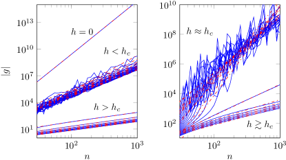
Figure 1: Scaling of $|g|$ for $\gamma=0.6$ and $h\in[0,0.8]$ (left) and for $\gamma=0.5$ and $h\in[0.735,0.755]$ (right). In both cases $\Gamma_{L}^{+}=0.3$, $\Gamma_{L}^{-}=0.5$, $\Gamma_{R}^{+}=0.1$, $\Gamma_{R}^{-}=0.5$. Blue curves represent the numerical data, while red lines are linear fits, whose results are summarized in Table 1. $|g|$ slightly fluctuates as a function of $n$ in the LRMC phase and the relative amplitude of the fluctuations increases close to the critical field $h_{c}$. Due to finite size effects and to the differential nature of the geometric tensor, the value where $|g|$ takes its maximum is slightly smaller than $h_{c}$, and this difference depends on $n$.

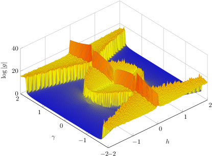
Figure 2: Maximum eigenvalue $|g|$ of the fidelity metric (2) for $n=250$. The Lindblad parameters are the same of Fig. 1. The larger value of $|g|$ close to the phase transition line $h=h_{c}(\gamma)$ is not evident in Fig. 2 because of the numerical mesh and because, the actual values of $|g|$ for $h\approx h_{c}$ can be comparable to those of the LRMC phase, depending on $n$ (e.g. see Fig. 1). The qualitative form of Fig. 2 is not affected by different values of the Lindblad parameters $\Gamma_{L,R}^{\pm}$ and by the dimension $n$.

The findings discussed in the above demonstrate that the metric tensor $g$, being directly linked to the correlations properties of the Gaussian NESS, encodes all the relevant information about the dissipative phase transition featured by the model (8); in particular, the specificity of the different phases (SRMC vs LRMC), and the information about the physical relevant parameters, being them the magnetic field or the anisotropy, that drive the different transitions are properly accounted for. As shown in Fig. (2), the complete phase diagram can indeed be reconstructed with the study of the single function $g$. While these results are specific to the model examined, the connection established in (2) roots the behaviour of $g$ in the correlations properties of the general class of GF-states. Accordingly, one expects the fidelity approach to have a broader scope of application. We would like to stress that there are compelling questions that are still unanswered. In the first place the relation between $g$ and other relevant quantities that have been used so far to characterize NESS-QPT; For the model (8), these are the range of correlations, and the finite-size scaling of Liouvillean gap $\Delta.$ The latter does not entirely capture the criticality phenomenon, and further investigation of the relation between criticality in NESS-QPT and geometrical and dynamical aspects is in order Poulin (2010). Notice also, that, in the XY model, different type of symmetries (discrete vs. continuous) are broken moving away from the $h=0$ or $\gamma=0$ line. It would be interesting to understand whether the scaling exponents of $ds^{2}$ at different lines can be related to different non-equilibrium universality classes. Extending the present results to non-Gaussian states de Melo et al. (2013) and transitions Prosen and Žnidarič (2010) is also an important future direction.

Translationally invariant case:–  In order to support the generality of the geometric approach in understanding dissipative phase transitions we apply our theoretical framework to a different dissipative model, first introduced in Horstmann et al. (2013). We consider an XY spin chain on a ring where each site is coupled to the environment via $L_{i}^{+}{=}\sqrt{\Gamma^{+}}f_{i}^{\dagger}$, $L_{i}^{-}{=}\sqrt{\Gamma^{-}}f_{i}$. The closed boundary conditions and the uniform interaction with the environment make the phase diagram very different from the previous one. Indeed, in this particular translationally invariant case, the critical points match the known values for GS-QPT: for $\gamma\neq 0$ there is a critical field $h=1$, while in the XX case the whole segment $|h|<1$ is critical. In the SM we have proved that the $|g|=O(n^{2})$ for the critical values and $|g|=O(n)$ elsewhere. The information-geometric content of this dissipative phase transition is not as rich as the one in Table. 1, and again the scaling of the metric tensor allows one a precise mapping of the phase-diagram.

Conclusions:–  In this Letter we developed an information-geometric framework for studying dissipative critical phenomena exhibit by the non-equilibrium steady states of Markovian evolutions described by quadratic Fermionic Liouvillean. We first derived a general formula for the infinitesimal Bures distance between Gaussian Fermionic (mixed) states. This in turn allows one to define a metric tensor $g$ on the manifold of steady states corresponding to different sets of control parameters. The intuitive idea underlying is that a transition between two structurally different phases should be reflected by the statistical distinguishability of pairs of infinitesimally close steady states. The method does not require the knowledge or the existence of any order parameters, as the tensor $g$ is directly connected to the two-point correlation functions which define the Gaussian Fermionic steady states. We have shown that a superextensive behaviour of the tensor $g$, implies some singularity for $n{\to}\infty$ in the derivative of the correlation functions. We have applied the method to specific (XY) models and shown that the scaling of the geometric tensor enables one to identify both the critical lines and to distinguish between different phases characterized by short or long ranged correlations. The metric tensor encodes also for the direction of maximal distinguishability in the parameter manifold, thus allowing a detailed study of the sensitivity of the steady state to small variations of some control parameters. This is a crucial point for experimental applications of dissipative evolution. The scope of the information-geometric approach extends well beyond the important quadratic case analzyed in this paper and may pave the way to the systematic study of general non-equilibrium critical phenomena. This in turn would allow the investigation of a broad class of systems and processes which are natural candidates for the preparation of desired quantum states and realization of quantum protocols.

Acknowledgements:–  P.Z. was supported by the ARO MURI grant W911NF-11-1-0268 and by NSF grant numbers PHY- 969969 and PHY-803304.

Supplementary Material

I Proof of Eq. (1)

We consider a Gaussian Fermionic state written in the following form

$$\rho=e^{-\frac{i}{4}\sum_{ij}G_{ij}\,w_{i}w_{j}}/Z~{},$$ (9)

where the matrix $G$ has to be real and antisymmetric. Accordingly $G$ can be cast in the canonical form by an orthogonal matrix $Q$, i.e.

$$G =Q^{T}\,\bigoplus_{k=1}^{n}\begin{pmatrix}0&g_{k}\\ -g_{k}&0\end{pmatrix}\,Q Q^{T}=Q^{-1}~{},$$ (10)

and has eigenvalues $\pm ig_{k}$. Moreover let $z_{i}=\sum_{j}Q_{ij}w_{j}$ be the new Majorana operators. Hence

$$\rho =\frac{1}{Z}\prod_{k}\left[\cosh\left(\frac{g_{k}}{2}\right)-i\sinh\left(\frac{g_{k}}{2}\right)\,z_{2k-1}z_{2k}\right]~{},$$ (11)

$$Z =\prod_{k}2\cosh\left(\frac{g_{k}}{2}\right)=\sqrt{\det\left[2\cosh\left(i\frac{G}{2}\right)\right]}~{},$$ (12)

where we used the fact that the eigenvalues of $iG$ are $\pm g_{k}$. As $C_{ij}=\frac{1}{2}\langle{[w_{i},w_{j}]}\rangle=\frac{2i}{Z}\frac{\partial Z}{\partial G_{ij}}$ one can show that

$$C=\tanh\left(i\frac{G}{2}\right)~{}.$$ (13)

The correlation matrix $C=C^{\dagger}=-C^{T}$ is diagonal in the same basis of $G$ and its eigenvalues read $c_{k}=\tanh(g_{k}/2)$. Hence

$$\rho =\prod_{k}\frac{1-ic_{k}\,z_{2k-1}z_{2k}}{2}~{},$$ (14)

where $|c_{k}|\leq 1$. Note that for $c_{k}=\pm 1$, one has $g_{k}=\pm\infty$, making the ansatz (9) not well defined, unlike Eq. (14). The latter possibility occurs for instance for pure states, as it is clear from the following explicit expression for the purity of the states (9) and the states (9) and (14):

$$\operatorname*{Tr}[\rho^{2}]=\frac{\det\left[2\cosh\left(i\,G\right)\right]^{\frac{1}{2}}}{\det\left[2\cosh\left(i\frac{G}{2}\right)\right]}=\sqrt{\det\left(\frac{1+C^{2}}{2}\right)}~{}.$$ (15)

We now derive the proof of Eqs. (1) and (2), dividing the different steps into three lemmas. At first we assume $c_{k}\neq\pm 1$ and then we extend the result for including pure states.

Lemma 1.

Let $\rho,\rho^{\prime}$ two GF-states (9) parametrized by $G,G^{\prime}$ respectively. Then

$$\mathcal{F}(\rho,\rho^{\prime}) =\operatorname*{Tr}\sqrt{\sqrt{\rho}\rho^{\prime}\sqrt{\rho}}$$ (16)

$$=\frac{\det\left[\openone+\sqrt{e^{iG/2}e^{iG^{\prime}}e^{iG/2}}\right]^{\frac{1}{2}}}{\det\left[\openone+e^{iG}\right]^{\frac{1}{4}}\,\det\left[\openone+e^{iG^{\prime}}\right]^{\frac{1}{4}}}~{}.$$ (17)

Proof.

This lemma is a direct consequence of the fact the quadratic Majorana operators form a Lie algebra:

$$\left[\frac{\boldsymbol{\mathbf{w}}\cdot A\boldsymbol{\mathbf{w}}}{4},\frac{\boldsymbol{\mathbf{w}}\cdot B\boldsymbol{\mathbf{w}}}{4}\right]=\frac{\boldsymbol{\mathbf{w}}\cdot\left[A,B\right]\boldsymbol{\mathbf{w}}}{4}~{},$$ (18)

and accordingly

$$e^{\frac{i}{4}\boldsymbol{\mathbf{w}}\cdot A\boldsymbol{\mathbf{w}}}e^{\frac{i}{4}\boldsymbol{\mathbf{w}}\cdot B\boldsymbol{\mathbf{w}}} =e^{\frac{i}{4}\boldsymbol{\mathbf{w}}\cdot D\boldsymbol{\mathbf{w}}}~{}, e^{A}\,e^{B}=e^{D}~{}.$$ (19)

Thanks to the above identity

$$\sqrt{\sqrt{\rho}\rho^{\prime}\sqrt{\rho}}\propto\exp\left(\frac{1}{4}\sum_{ij}\left(\frac{\log\left[e^{-iG/2}e^{-iG^{\prime}}e^{-iG/2}\right]}{2}\right)_{ij}\,w_{i}w_{j}\right)~{},$$ (20)

and using (12) we find

$$\mathcal{F}(\rho,\rho^{\prime})=\frac{\det\left[\cosh\left(\frac{1}{4}\log e^{-iG/2}e^{-iG^{\prime}}e^{-iG/2}\right)\right]^{\frac{1}{2}}}{\sqrt{\det\left[\cosh\left(i\frac{G}{2}\right)\right]^{\frac{1}{2}}\,\det\left[\cosh\left(i\frac{G^{\prime}}{2}\right)\right]^{\frac{1}{2}}}}~{},$$ (21)

which is equivalent to (17). ∎

A convenient parametrization of Eq. (17) is obtained in terms of the correlation function by defining the new matrix $T=e^{iG}$. Then

$${C=\frac{T-\openone}{T+\openone}}~{}, T^{T}=T^{-1}~{},T^{\dagger}=T~{},$$ (22)

$$\mathcal{F}(\rho,\rho^{\prime})=:\mathcal{F}(T,T^{\prime})=\frac{\det\left[\openone+\sqrt{\sqrt{T}\,T^{\prime}\sqrt{T}}\right]^{\frac{1}{2}}}{\det\left[\openone+T\right]^{\frac{1}{4}}\,\det\left[\openone+T^{\prime}\right]^{\frac{1}{4}}}~{}.$$ (23)

The following lemma conveys the metric pull back with in the manifold of states parametrized by $T$:

Lemma 2.

Let $ds^{2}=8\,ds^{2}_{B}=16[1-\mathcal{F}(T,T+dT)]$ the fidelity metric around the state (9) pulled back in the space of the matrices $T$ and let $dT=\partial_{\mu}T\,d\lambda_{\mu}$ where $\lambda_{\mu}\in\mathcal{M}$ are the parameters of the model. Then the fidelity metric can be cast into the form $ds^{2}=\sum_{\mu\nu}g_{\mu\nu}\,d\lambda_{\mu}\,d\lambda_{\nu}$ where the geometric tensor is

$$g_{\mu\nu}=2\sum_{ij}\frac{(\partial_{\mu}T)_{ij}\,(\partial_{\nu}T)_{ji}}{(1+t_{i})(1+t_{j})(t_{i}+t_{j})}~{}.$$ (24)

In (24) the sum is performed in the basis in which $T$ is diagonal, i.e. we set $T=\sum_{i}t_{i}|{i}\rangle\langle{i}|$ and $(\partial_{\mu}T)_{ij}=\langle{i}|\partial_{\mu}T|{j}\rangle$.

Proof.

Proceeding along the same lines of Section 3 of Sommers and Zyczkowski (2003) we obtain for $T^{\prime}=T+dT$

$$\sqrt{\sqrt{T}T^{\prime}\!\sqrt{T}}=T+\sum_{ij}|{i}\rangle\langle{j}|\,\frac{\sqrt{t_{i}t_{j}}}{t_{i}+t_{j}}\,dT_{ij}-$$ (25)

$$-\sum_{ijk}|{i}\rangle\langle{k}|\,dT_{ij}dT_{jk}\,\frac{\sqrt{t_{i}t^{2}_{j}t_{k}}}{(t_{i}+t_{j})(t_{j}+t_{k})(t_{i}+t_{k})}+\mathcal{O}\left(dT\right)^{3}$$

Owing to the above expression and to Eq.(23) the fidelity $\mathcal{F}(T,T+dT)$ can be written in terms of some infinitesimal operators $\delta,\partial$

$$\mathcal{F}(T,T+dT) \simeq\frac{\det\left[(\openone+T)(\openone+\partial)\right]^{\frac{1}{2}}}{\det\left[\openone+T\right]^{\frac{1}{4}}\,\det\left[(\openone+T)(\openone+\delta)\right]^{\frac{1}{4}}}$$

$$=\frac{\det\left[\openone+\partial\right]^{\frac{1}{2}}}{\det\left[\openone+\delta\right]^{\frac{1}{4}}}=e^{\frac{1}{2}\operatorname*{Tr}\log(1+\partial)-\frac{1}{4}\operatorname*{Tr}\log(1+\delta)}$$

$$\simeq e^{\frac{1}{2}\operatorname*{Tr}\left(\partial-\delta/2\right)-\frac{1}{4}\operatorname*{Tr}\left(\partial^{2}-\delta^{2}/2\right)}~{},$$ (26)

where

$$\delta =(1+T)^{-1}\,dT=\sum_{ij}|{i}\rangle\langle{j}|\,\frac{1}{1+t_{i}}\,dT_{ij}~{},$$ (27)

$$\partial =(1+T)^{-1}\,\left(\sqrt{\sqrt{T}T^{\prime}\!\sqrt{T}}-T\right)$$ (28)

$$=\sum_{ij}|{i}\rangle\langle{j}|\,\frac{\sqrt{t_{i}t_{j}}}{t_{i}+t_{j}}\,\frac{1}{1+t_{i}}\,dT_{ij}-$$

$$-\sum_{ijk}|{i}\rangle\langle{k}|\,dT_{ij}dT_{jk}\,\frac{\sqrt{t_{i}t^{2}_{j}t_{k}}}{(t_{i}+t_{j})(t_{j}+t_{k})(t_{i}+t_{k})}\,\frac{1}{1+t_{i}}~{}.$$

The elements of Eq. (26) become

$$\operatorname*{Tr}(\partial-\delta/2) =-\frac{1}{4}\sum_{ij}\left|dT_{ij}\right|^{2}\,\frac{1}{(t_{i}+t_{j})^{2}}\,\left(\frac{t_{j}}{1+t_{i}}+\frac{t_{i}}{1+t_{j}}\right)~{},$$ (29)

$$\operatorname*{Tr}\delta^{2} =\sum_{ij}\left|dT_{ij}\right|^{2}\,\frac{1}{(1+t_{i})(1+t_{j})}~{},$$ (30)

$$\operatorname*{Tr}\partial^{2} \simeq\sum_{ij}\left|dT_{ij}\right|^{2}\,\frac{t_{i}t_{j}}{(t_{i}+t_{j})^{2}}\,\frac{1}{(1+t_{i})(1+t_{j})}~{},$$ (31)

so that

$$\mathcal{F}(T,T+dT)\simeq 1-\frac{1}{8}\sum_{ij}\frac{\left|dT_{ij}\right|^{2}}{(1+t_{i})(1+t_{j})(t_{i}+t_{j})}~{},$$ (32)

which completes the proof. ∎

Before proving Eq. (1) we introduce the following lemma which will be used for analytical continuations to the pure state manifold:

Lemma 3.

Let $f(x,y):=(x-y)^{2}(1-xy)^{-1}$ be a function defined in $[-1,\,1]^{2}-\{z^{+},\,z^{-}\},\,z^{\pm}:=(\pm 1,\,\pm 1).$ Then $f(x,\,y)\leq 4$ and $\lim_{(x,y)\to z^{\pm}}f(x,\,y)=0$.

Proof.

The upper bound is found thanks to $1-xy=1-[(x+y)^{2}-(x-y)^{2}]/4\geq(x-y)^{2}/4$. In order to show that $\lim_{(x,y)\to z^{\pm}}f(x,\,y)=0$ let us restrict $f$ to the $x\geq 0,\,y\geq 0$ part of the domain to analyse the limit to $z^{+}$. The limit $z^{-}$ follows because of the $(x,\,y)\to(-x,\,-y)$ symmetry of $f.$ One can write $y=1+m\,(x-1)$ or $x=1+m\,(y-1)$ with with $m\in[0,\,1].$ Because of the $(x,\,y)\to(y,\,x)$ symmetry of $f$ we can consider just the first case. One obtains $f(x,y)=(1-x)\frac{(1-m)^{2}}{1+mx}\leq 1-x$ this quantity in a disk of radius $\delta$ centered on $z^{+}$ is upper bounded by $\delta$. This shows that $\forall\epsilon>0,\,\exists\delta=\delta(\epsilon)$ s.t $\|(x,\,y)-z^{+}\|\leq\delta\Rightarrow f(x,\,y)\leq\epsilon$ (with $\delta(\epsilon)=\epsilon$), i.e., the claim. ∎

Proof of Eq. (1).

Eq. (2) is obtained directly from lemma 2. Indeed, from Eq. (22)

$$dC=dT\frac{1}{1+T}-\frac{T-1}{T+1}\,dT\,\frac{1}{T+1}=2\frac{1}{T+1}dT\frac{1}{T+1}~{}.$$ (33)

Inserting the above equation in (24), and noting that $C$ and $T$ are diagonal in the same basis, $c_{i}=\frac{t_{i}-1}{t_{i}+1}$, one obtains

$$g_{\mu\nu}=\sum_{ij}\frac{(\partial_{\mu}C)_{ij}\,(\partial_{\nu}C)_{ji}}{1-c_{i}c_{j}}~{}.$$ (34)

The singular behaviour of (34) for $c_{i}=\pm 1$ is just apparent. Indeed, let $iG|j\rangle=g_{j}|j\rangle\,(j=1,\ldots,2n),\,{\rm{Sp}}(iG)=\{g_{j}\}\subset{\mathbf{R}}$ then $C=\sum_{j}c_{j}|j\rangle\langle j|,\,c_{j}:=\tanh(g_{j}/2).$ By differentiation $dC=\sum_{j}\left((1-c_{j}^{2})\frac{dg_{j}}{2}|j\rangle\langle j|+c_{j}(|dj\rangle\langle j|+|j\rangle\langle dj|)\right).$ One has therefore the following matrix elements $(dC)_{jj}=(1-c_{j}^{2})dg_{j}$ and $(dC)_{ij}=(c_{i}-c_{j})\langle di|j\rangle,\,(i\neq j).$ Plugging these in (34)

$$ds^{2}=\frac{1}{4}\sum_{j}(1-c_{j}^{2})\,dg_{j}^{2}+\sum_{i\neq j}f(c_{i},c_{j})\,|\langle di|j\rangle|^{2}~{}.$$ (35)

Now one sees easily that for $c_{j}\to\pm 1$ the first (diagonal) contribution in (35) vanishes while the second, thanks to lemma 3, is upper bounded by $4\,\sum_{i\neq j}|\langle di|j\rangle|^{2}$ for all $c_{i},c_{j}\in(-1,\,1)$ and vanishes for $(c_{i},c_{j})\to z^{\pm}$: even if (34) has been derived for $C$ such that $c_{i}\neq\pm 1$, we can perform the limit $|c_{i}|\to 1,(\forall i)$ and, in this way, extend the metric to the pure state manifold just by setting $c_{i}c_{j}$ to $-1$ (as for the case $c_{i}c_{j}=1$ gives vanishing contribution).

The basis independent expression Eq. (1) follows from (34)

$$ds^{2}=\sum_{\mu\nu}g_{\mu\nu}d\lambda_{\mu}d\lambda_{\nu}=\langle({\mathbf{1}}-{\rm{Ad}}C)^{-1}(dC),\,dC\rangle$$ (36)

where $dC=\sum_{\mu}d\lambda_{\mu}\partial_{\mu}C,$ and ${\rm{Ad}}C(X):=CXC^{\dagger}=CXC=(L_{C}\circ R_{C})(X)$ is the adjoint action. To see this let us first write $dC=\sum_{ij}(dC)_{ij}|i\rangle\langle j|$ where $C|i\rangle=c_{i}|i\rangle.$ Then $(1-{\rm{Ad}}C)^{-1}(dC)=\sum_{ij}(dC)_{ij}(1-c_{i}c_{j})^{-1}\,|i\rangle\langle j|$ and $\langle(1-{\rm{Ad}}C)^{-1}(dC),\,dC\rangle=\sum_{ij}{(dC)_{ij}}^{*}(1-c_{i}c_{j})^{-1}\langle|i\rangle\langle j|,\,dC\rangle=\sum_{ij}{(dC)_{ij}}^{*}(dC)_{ij}(1-c_{i}c_{j})^{-1}.$ The zero contribution to the sum (34) for $c_{i}c_{j}=1$ is considered thanks to the pseudo-inverse. ∎

One can show that Eq. (1) reduces to the known expressions when $\rho$ is a thermal state Zanardi et al. (2007b) and when $\rho$ is a pure state Cozzini et al. (2007), provided that the appropriate matrices $T$ or $C$ are used. In the next section, this theorem is applied to NESS-QPT where $C$ is given by the solution of the Sylvester equation (5).

II Liouvillean steady state

We call $\mathcal{R}$ the $4^{n}$-dimensional operator spaces generated by $\prod_{j}w_{j}^{s_{j}}$, ($s_{j}\in\{0,1\}$), and we use the notation $|{\boldsymbol{\mathbf{s}}})$ for referring to the elements of $\mathcal{R}$, normalized with respect to the Hilbert-Schmidt inner product, i.e. $({\boldsymbol{\mathbf{s}}}|{\boldsymbol{\mathbf{s}}})\equiv\operatorname*{Tr}[s^{\dagger}s]=1$ for $|{\boldsymbol{\mathbf{s}}})\in\mathcal{R}$.

Following the notation introduced in the Letter, the Liouvillean $\mathcal{L}\colon\mathcal{R}\rightarrow\mathcal{R}$ introduced in (3) can be written as

$$\mathcal{L}=-\frac{1}{2}\begin{pmatrix}{\boldsymbol{\mathbf{a}}}^{\dagger}&\boldsymbol{\mathbf{a}}\end{pmatrix}\,\begin{pmatrix}X&Y\\ 0&-X^{T}\end{pmatrix}\,\begin{pmatrix}\boldsymbol{\mathbf{a}}\\ {\boldsymbol{\mathbf{a}}}^{\dagger}\end{pmatrix}-\frac{1}{2}\operatorname*{Tr}X~{}.$$ (37)

The superoperator $a_{j}^{\dagger}$ is the Hermitian conjugate of $a_{j}$ in $\mathcal{R}$.

If $C$ is the matrix solution of (5) then

$$\begin{pmatrix}X&Y\\ 0&-X^{T}\end{pmatrix}=\begin{pmatrix}U&-C\,U^{-T}\\ 0&U^{-T}\end{pmatrix}\,\begin{pmatrix}x&0\\ 0&-x\end{pmatrix}\,\begin{pmatrix}U^{-1}&U^{-1}\,C\\ 0&U^{T}\end{pmatrix}~{}.$$ (38)

We show now that the latter transformation is non-unitary Bogoliubov transformation Blaizot and Ripka (1986) and that everything is consistent. It is known that non-unitary Bogoliubov transformations are isomorphic to the group of orthogonal complex matrices $O(4n,\mathbb{C})$. This condition can be expressed in a simple way thanks to Eq.(2.6) of Blaizot and Ripka (1986), i.e.

$$\hat{V}\,\Sigma^{x}\,\hat{V}^{T} =\Sigma^{x}~{}, \Sigma^{x} =\sigma^{x}\otimes\openone_{2n}~{}.$$ (39)

It is simple to show that the transformation $\hat{V}$

$$\hat{V} =\begin{pmatrix}U^{-1}&U^{-1}\,C\\ 0&U^{T}~{},\end{pmatrix}$$ (40)

satisfies that condition. We define new diagonal creation and annihilation operators as

$$\begin{pmatrix}\boldsymbol{\mathbf{d}}\\ {\boldsymbol{\mathbf{d}}}^{\times}\end{pmatrix} =\hat{V}\,\begin{pmatrix}\boldsymbol{\mathbf{a}}\\ {\boldsymbol{\mathbf{a}}}^{\dagger}\end{pmatrix}~{}.$$ (41)

Since $\mathcal{V}$ is a non-unitary Bogoliubov transformation the operators $d_{i}$ and $d_{j}^{\times}$ satisfy the CAR-algebra, but $d_{j}^{\times}\neq d_{j}^{\dagger}$. Moreover, using $\begin{pmatrix}{\boldsymbol{\mathbf{a}}}^{\dagger}&\boldsymbol{\mathbf{a}}\end{pmatrix}=\begin{pmatrix}\boldsymbol{\mathbf{a}}\\ {\boldsymbol{\mathbf{a}}}^{\dagger}\end{pmatrix}^{T}\,\Sigma^{x}$ then it is simple to show that

$$\mathcal{L}=-\frac{1}{2}\begin{pmatrix}{\boldsymbol{\mathbf{d}}}^{\times}&\boldsymbol{\mathbf{d}}\end{pmatrix}\,\begin{pmatrix}x&0\\ 0&-x\end{pmatrix}\,\begin{pmatrix}\boldsymbol{\mathbf{d}}\\ {\boldsymbol{\mathbf{d}}}^{\times}\end{pmatrix}-\frac{1}{2}\operatorname*{Tr}X~{},$$ (42)

i.e.,

$${\mathcal{L}=-\sum_{j}x_{j}\,d^{\times}_{j}\,d_{j}}~{}.$$ (43)

Note also that the transformation (41) can be written thanks to Eq (2.16) of Blaizot and Ripka (1986) into the form

$$d_{j} =\mathcal{V}\,a_{j}\,\mathcal{V}^{-1}~{}, d_{j}^{\times} =\mathcal{V}\,a_{j}^{\dagger}\,\mathcal{V}^{-1}~{},$$ (44)

where

$$\mathcal{V}=:\exp\left(-\frac{1}{2}{\boldsymbol{\mathbf{a}}}^{\dagger}\,C\,{\boldsymbol{\mathbf{a}}}^{\dagger}+{\boldsymbol{\mathbf{a}}}^{\dagger}\,(U-1)\,{\boldsymbol{\mathbf{a}}}\right):~{},$$ (45)

and $:\exp(\cdot):$ refers to the normal ordering of the exponential.

It is now possible to express the stationary state of the Liouvillean, i.e. the state $\Omega$ such that $\mathcal{L}\Omega=0$, as the ${\boldsymbol{\mathbf{d}}}$-vacuum, i.e. $d_{j}|{\Omega})=0$. The identity operator, i.e. the element $|{\boldsymbol{\mathbf{0}}})\in\mathcal{R}$ is the $\boldsymbol{\mathbf{a}}$-vacuum, i.e. $a_{i}|{\boldsymbol{\mathbf{0}}})=0$, $\forall j=1,\ldots 2n$, and in particular $({\boldsymbol{\mathbf{0}}}|\mathcal{L}=0$. The $\boldsymbol{\mathbf{d}}$-vacuum can be readily obtained from the Bogoliubov transformation: $|{\Omega})=\mathcal{V}|{\boldsymbol{\mathbf{0}}})$. Indeed, as $a_{j}|{\boldsymbol{\mathbf{0}}})=0$, one has $d_{j}|{\Omega})=\mathcal{V}a_{j}\mathcal{V}^{-1}\mathcal{V}|{\boldsymbol{\mathbf{0}}})=0$. Hence,

$$|{\Omega})=\mathcal{V}|{\boldsymbol{\mathbf{0}}})=e^{-\frac{1}{2}{\boldsymbol{\mathbf{a}}}^{\dagger}\,C\,{\boldsymbol{\mathbf{a}}}^{\dagger}}|{\boldsymbol{\mathbf{0}}})~{}.$$ (46)

We now show that the state (46) is exactly (14). Thanks to the transformation $Q$ defined in (10) and the direct relation (13) one can write the imaginary antisymmetric matrix $C=Q^{T}\,\bigoplus_{k}\begin{pmatrix}0&ic_{k}\\ -ic_{k}&0\end{pmatrix}\,Q$. Then, using the definition (46)

$$\frac{1}{2}{\boldsymbol{\mathbf{a}}}^{\dagger}\,C\,{\boldsymbol{\mathbf{a}}}^{\dagger}\rho =\frac{1}{8}\left(\boldsymbol{\mathbf{w}}\cdot C\boldsymbol{\mathbf{w}}\rho+2\boldsymbol{\mathbf{w}}\cdot C\rho\boldsymbol{\mathbf{w}}+\rho\boldsymbol{\mathbf{w}}\cdot C\boldsymbol{\mathbf{w}}\right)$$

$$=\frac{i}{4}\sum_{k}c_{k}\big{[}z_{2k-1}z_{2k}\rho+z_{2k-1}\rho z_{2k}-$$

$$\quad\quad\quad\quad-z_{2k}\rho z_{2k-1}+\rho z_{2k-1}z_{2k}\big{]}$$

$$=:\sum_{k}\mathcal{G}_{k}(\rho)~{}.$$ (47)

As

$$\mathcal{G}_{k}(\openone) =i\,c_{k}\,z_{2k-1}z_{2k}~{}, \mathcal{G}_{k}(z_{2k-1}z_{2k})=0~{},$$ (48)

it is clear that

$$\Omega\propto e^{-\frac{1}{2}c^{\dagger}Cc^{\dagger}}|{0})\propto\prod_{k}e^{-\mathcal{G}_{k}}\openone=\prod_{k}\left(1-i\,c_{k}\,z_{2k-1}z_{2k}\right)~{},$$ (49)

thus recovering Eq.(9).

The conditions for the existence and uniqueness of (49) are given in Prosen (2010). We now study those conditions and express them in terms of the spectral gap. The correlation matrix matrix $C\in M_{2n}(\mathbf{C})$ is the matrix solution of Eq. (5). To study the solution of that equation it is useful to consider the (non-canonical) “vectorising” isomorphism $\phi\colon M_{2n}({\mathbf{C}})\rightarrow({\mathbf{C}}^{2n})^{\otimes\,2}\,/\,|i\rangle\langle j|\rightarrow|i\rangle\otimes|j\rangle.$ This is also a Hilbert-space isomorphism, namely $\langle\phi(A),\phi(B)\rangle=\langle A,\,B\rangle={\rm{Tr}}\,(A^{\dagger}B).$ One can directly check that if $R_{X}(C):=CX$ and $L_{X}(C):=XC$ then $\phi(R_{X}(C))=(\phi\circ R_{X}\circ\phi^{-1}\circ\phi)(C)=({\mathbf{1}}\otimes X^{T})\phi(C),$ and $\phi(L_{X}(C))=(\phi\circ L_{X}\circ\phi^{-1}\circ\phi)(C)=(X\otimes{\mathbf{1}})\phi(C).$ Applying $\phi$ to both sides of (5) one then obtains ($\tilde{C}:=\phi(C),\,\tilde{Y}:=\phi(Y)$)

$$(X\otimes{\mathbf{1}}+{\mathbf{1}}\otimes X)\tilde{C}=:\hat{X}\tilde{C}=\tilde{Y},$$ (50)

where $\tilde{C},\tilde{Y}\in({\mathbf{C}}^{2n})^{\otimes\,2},\,\hat{X}\in{\rm{End}}({\mathbf{C}}^{2n})^{\otimes\,2}\cong M_{4n^{2}}({\mathbf{C}}).$ There are three different key operators in the formalism for obtaining the steady state:

1. The Liouvillean ${\cal L}\colon{\rm{End}}(({\mathbf{C}}^{2})^{\otimes n})\rightarrow{\rm{End}}(({\mathbf{C}}^{2})^{\otimes n}),$ a $2^{2n}\times 2^{2n}$ matrix. Its complex spectrum, from (43), is given by

   $${\rm{Sp}}({\cal L})=-\{x_{\mathbf{n}}:=\sum_{j=1}^{2n}x_{j}n_{j}\,/\,n_{j}=0,1,\,x_{j}\in{\rm{Sp}}(X)\}.$$ (51)

   Notice that $0\in{\rm{Sp}}({\cal L})$ i.e., $\cal L$ is always non-invertible and that the steady state(e.g., our Gaussian one ${\mathbf{n}}={\mathbf{0}}$) are in the kernel of $\cal L$. If this latter is one-dimensional (unique steady state) the gap of $\cal L$ can be defined as ${\Delta}_{\cal L}:=\min_{{\mathbf{n}}\neq{\mathbf{0}}}\,|x_{\mathbf{n}}|.$

2. The map $X\colon{\mathbf{C}}^{2n}\rightarrow{\mathbf{C}}^{2n},$ a $2n\times 2n$ real diagonalizable matrix. Its spectrum is $\{x_{j}\}_{j=1}^{2n}\subset{\mathbf{C}}$ and (because of reality) is invariant under complex conjugation. On physical grounds (stability) we must have $\Re\,x_{j}\geq 0,\forall j.$ Indeed, the time-scale for convergence $\rho(t)\to\rho(\infty)$ is dictated by $\tilde{\Delta}^{-1}$ where $\tilde{\Delta}=\min_{{\mathbf{n}}\neq{\mathbf{0}}}\Re\,x_{{\mathbf{n}}}.$

3. The map $\hat{X}=X\otimes{\mathbf{1}}+{\mathbf{1}}\otimes X\colon{\mathbf{C}}^{2n}\otimes{\mathbf{C}}^{2n}\rightarrow{\mathbf{C}}^{2n}\otimes{\mathbf{C}}^{2n},$ a $4n^{2}\times 4n^{2}$ matrix. It spectrum is $\{x_{i}+x_{j}\}_{i,j=1}^{2n}\subset{\mathbf{C}}$ and the minimum (in modulus) is given by $\Delta_{\hat{X}}:=\min_{i,j}|x_{i}+x_{j}|.$ Note also that

   $$\Delta_{\hat{X}}^{-1}=\|\hat{X}^{-1}\|_{\infty}~{}.$$ (52)

   For the uniqueness of the steady state we must have $\hat{X}$ invertible i.e., $\Delta_{\hat{X}}>0.$

Proposition 1.

If $\Delta=\min_{j}2\Re(x_{j})>0$ then

$$\Delta={\Delta}_{\cal L}=\Delta_{\hat{X}}~{}.$$ (53)

Proof.

$|x_{\mathbf{n}}|=|\sum_{j=1}^{2n}x_{j}n_{j}|\geq|\Re(\sum_{j=1}^{2n}n_{j}x_{j})|.$ The first bound can be saturated by choosing the $n_{j}$’s in such a way that only a set $P$ of complex conjugated pairs $x^{\pm}_{p}$ of eigenvalues are present. In this case $|\Re(\sum_{j=1}^{2n}n_{j}x_{j}|=2\sum_{p\in P}\Re\,x_{p}.$ Where we used the assumption $(\forall p)\,\Re\,x_{p}\geq 0.$ Using again positivity of all the terms, this sum can be made as small as possible by choosing $|P|=1$ and minimizing over $p=1,\ldots,n.$ This shows that ${\Delta}_{\cal L}=\min_{\mathbf{n}}|x_{\mathbf{n}}|=2\min\{\Re\,x_{p}\}_{p=1}^{n}.$ It is clear now that a similar argument shows that $\Delta_{\hat{X}}=\min\{|x_{i}+x_{j}|\}_{i,j=1}^{2n}$ is given by the same expression i.e. ${\Delta}_{\cal L}=\Delta_{\hat{X}}$. Finally $\Delta=2\min_{\mathbf{n}}\Re\,x_{\mathbf{n}}\equiv 2\tilde{\Delta}=2\min_{p}\Re\,x_{p}=\Delta_{\cal L}$. ∎

III Non-diagonalizable case

The non-diagonalizable case has been extensively handled in Prosen (2010). In the previous section we have assumed $X$ to be diagonalizable for simplicity, and because the matrices $X$ encountered in our numerical simulations were diagonalizable. Here we briefely discuss the general case. The matrix $X$ can always be put in the Jordan canonical form, i.e. $X=U\,x^{J}\,U^{-1}$ with $x^{J}=\oplus_{b}J_{\ell_{b}}(x_{b})$,

$$J_{\ell_{b}}(x_{b})=\begin{pmatrix}x_{b}&1&\\ &x_{b}&1&\\ &&x_{b}&1&\\ &&&\ddots&\ddots&\end{pmatrix}~{}:$$ (54)

$x_{b}$ are (possibly equal) eigenvalues of $X$ and $\ell_{b}$ is the dimension of the Jordan block: each block is composed of $\ell_{b}$ degenerate eigenvalues of $X$. The form of the transformation (40) remains the same (although with a new matrix $U$) while (43) becomes

$$\mathcal{L}=-\sum_{j=1}^{2n}x_{j}\,d_{j}^{\times}d_{j}-\sum_{b}\sum_{k=1}^{\ell_{b}-1}d^{\times}_{b_{k}+1}d_{b_{k}}~{},$$ (55)

where $b_{k}$ refers to the index of the $k$th element in the $b$th Jordan block. It is clear that the state (46) is still a stationary state. Moreover, in Prosen (2010) it has been shown that the spectrum of the Liuvillean is

$${\rm{Sp}}({\cal L})=-\{x_{\mathbf{n}}:=\sum_{b}x_{b}n_{b}\,/\,n_{b}=0,\cdots,\ell_{b}\}.$$ (56)

Accordingly, $\Delta_{\mathcal{L}}=\Delta\equiv 2\min_{b}\Re[x_{b}]$. If $\Delta>0$ the steady state (46) is unique Prosen (2010).

In the non-diagonalizable case the last equation in Eq. (53) is not satisfied. On the other hand one can obtain the following

Proposition 2.

$$\|\hat{X}^{-1}\|_{\infty}<\frac{1+p(\Delta^{-1})}{\Delta}~{},$$ (57)

for a certain polynomial $p()$.

Proof.

We start by writing

$$\hat{X} =\bigoplus_{b}J_{\ell_{b}}(x_{b})\otimes\openone+\bigoplus_{b}\openone\otimes J_{\ell_{b}}(x_{b})$$

$$=\bigoplus_{b,d}\left[J_{\ell_{b}}(x_{b})\otimes\openone_{\ell_{d}}+\openone_{\ell_{b}}\otimes J_{\ell_{d}}(x_{d})\right]$$

$$=\hat{x}+\bigoplus_{b,d}\left[J_{\ell_{b}}(0)\otimes\openone_{\ell_{d}}+\openone_{\ell_{b}}\otimes J_{\ell_{d}}(0)\right]~{},$$ (58)

where $\hat{x}$ is the diagonal matrix with entries $x_{i}+x_{j}$ and where we used the decomposition $\openone=\oplus_{b}1_{\ell_{b}}$. Moreover, thanks to Lemma 3.1 of Ref. Prosen (2010),

$$\hat{X} =\hat{x}+\bigoplus_{b,d}\bigoplus_{r=1}^{\min\{\ell_{b},\ell_{d}\}}J_{\ell_{b}+\ell_{d}-2r+1}(0)$$

$$=\hat{x}\left[\openone+\bigoplus_{b,d}\bigoplus_{r=1}^{\min\{\ell_{b},\ell_{d}\}}\frac{J_{\ell_{b}+\ell_{d}-2r+1}(0)}{x_{b}+x_{d}}\right]~{}.$$ (59)

As $J$ is nilpotent,

$$\hat{X}^{-1} =\hat{x}^{-1}\left[\openone+\bigoplus_{b,d}\bigoplus_{r=1}^{\min\{\ell_{b},\ell_{d}\}}\sum_{m=1}^{\ell_{b}+\ell_{d}-2r}\left(-\frac{J_{\ell_{b}+\ell_{d}-2r+1}(0)}{x_{b}+x_{d}}\right)^{m}\right]~{},$$

and

$$\|\hat{X}^{-1}\|_{\infty} \leq\|\hat{x}^{-1}\|_{\infty}\left[1+\max_{b,d}\max_{r}\sum_{m=1}^{\ell_{b}+\ell_{d}-2r}\frac{1}{|x_{b}+x_{d}|^{m}}\right]$$

$$=\|\hat{x}^{-1}\|_{\infty}\left[1+\max_{b,d}\sum_{m=1}^{\ell_{b}+\ell_{d}-2}\frac{1}{|x_{b}+x_{d}|^{m}}\right]$$

$$\leq\frac{1}{\Delta}\left[1+\max_{b,d}\sum_{m=1}^{\ell_{b}+\ell_{d}-2}\frac{1}{\Delta^{m}}\right]~{}.$$ (60)

∎

IV Upper bounds

In order to derive some bounds to the fidelity metric $ds^{2}$ let us express Eq. (1) in a convenient form thanks to the vectorization isomorphism. As ${\rm{Ad}}_{C}(X)=(L_{C}\circ R_{C})(X)$ one has $\phi\circ(L_{C}\circ R_{C})\circ\phi^{-1}=C\otimes C^{T}=-C^{\otimes\,2}$ and Eq. (1) becomes

$$ds^{2}=\langle({\mathbf{1}}+C^{\otimes\,2})^{-1}(d\tilde{C}),\,d\tilde{C}\rangle=\|({\mathbf{1}}+C^{\otimes\,2})^{-1/2}(d\tilde{C})\|^{2}~{},$$ (61)

where $d\tilde{C}=\phi(dC).$ Using the Cauchy-Schwarz inequality and the definition of operator norm one obtains

$$ds^{2} \leq\|({\mathbf{1}}+C^{\otimes\,2})^{-1}(d\tilde{C})\|\|d\tilde{C}\|\leq P_{C}\,\|d\tilde{C}\|^{2}$$

$$\leq 2nP_{C}\,\|d{C}\|^{2}_{\infty}~{},$$ (62)

where we have exploited the fact that, by construction, $\|\tilde{A}\|:=\|\phi(A)\|=\|A\|_{2}$ and $\|A\|_{2}\leq\sqrt{2n}\|A\|_{\infty}.$ Now ${\rm{Sp}}(C^{\otimes\,2})=\{c_{i}c_{j}\,/\,c_{i},c_{j}\in{\rm{Sp}}(C)\}$ and, from $C=-C^{T},$ the spectrum of $C$ is invariant under $c_{i}\rightarrow-c_{j},$ it follows that $\|({\mathbf{1}}+C^{\otimes\,2})^{-1}\|_{\infty}=(1+\min_{i,j}c_{i}c_{j})^{-1}=(1-\max_{i}c_{i}^{2})^{-1}=(1-\|C\|^{2}_{\infty})^{-1}$. The bound (62) is not specific to dissipative quadratic Liouvillean. In order to connect Eq.(62) with the properties of the Liouvillean (43) we differentiate Eq. (50)

$$d\tilde{C}=\hat{X}^{-1}d\tilde{Y}-\hat{X}^{-1}d\hat{X}\tilde{C}~{}.$$ (63)

As $d\equiv\sum_{\mu}d\lambda_{\mu}\partial_{\mu}$ the above equation can be conveniently calculated via

$$X\,\left(\partial_{\mu}C\right)+\left(\partial_{\mu}C\right)\,X^{T}=\partial_{\mu}Y-\left(\partial_{\mu}X\right)\,C-C\,\left(\partial_{\mu}X^{T}\right)~{},$$ (64)

i.e. the matrices $\partial_{\mu}C$ entering in (34) can be obtained by solving a new Sylvester equation where the matrices $X,Y,\partial_{\mu}X,\partial_{\mu}Y$ are given by the model. Taking norms in $({\mathbf{C}}^{2n})^{\otimes\,2}$

$$\|d\tilde{C}\| \leq\|\hat{X}^{-1}\|_{\infty}(\|d\tilde{Y}\|+\|d\hat{X}\|_{\infty}\|\tilde{C}\|)$$

$$=\|\hat{X}^{-1}\|_{\infty}(\|d{Y}\|_{2}+\|d\hat{X}\|_{\infty}\|{C}\|_{2})$$

$$\leq\sqrt{2n}\|\hat{X}^{-1}\|_{\infty}(\|d{Y}\|_{\infty}+\|d\hat{X}\|_{\infty}\|{C}\|_{\infty})$$

$$\leq\sqrt{2n}\|\hat{X}^{-1}\|_{\infty}(\|d{Y}\|_{\infty}+\|d\hat{X}\|_{\infty})~{},$$ (65)

where, among other things, we used the inequality $\|C\|_{\infty}\leq 1$ which follows from the anstaz (13). In summary we have the following upper bound on the squared Hibert-Schmidt norm of $dC$ in terms of the control parameters and their differentials i.e., $X,\,dX$ and $Y,\,dY$

$$\|d\tilde{C}\|^{2}\leq 2n\|\hat{X}^{-1}\|_{\infty}^{2}(\|d{Y}\|_{\infty}+2\|d{X}\|_{\infty})^{2}$$ (66)

where we also used $\|d\hat{X}\|_{\infty}=\|dX\otimes{\mathbf{1}}+{\mathbf{1}}\otimes dX\|_{\infty}\leq 2\|dX\|_{\infty}$. Pluggin the above equation in (62) and using Proposition 1 one then obtains the bound (7).

Note that in the non-diagonalizable case there is a correction to Eq. (7) due to the polynomial $p$ in (57). However, this correction does not alter the main conclusion of bound (7): a superextensive behaviour of $ds^{2}$ implies the closing of the Liuvillean gap.

V Application II: translationally invariant case

In this section we study a simpler model where all the informations about the phase transition can be obtained analytically. The model consists of a fermionic chain on a ring described the Hamiltonian

$$H=\sum_{i=i}^{n}\left(f_{i}^{\dagger}f_{i+1}+\gamma f_{i}^{\dagger}f_{i+1}^{\dagger}+hf_{i}^{\dagger}f_{i}\right)+\text{h.c.}~{}.$$ (67)

Owing to the Jordan-Wigner transformation, the above model can be mapped into the XY spin model (8), though with closed boundary conditions. The interaction with the environment is described by the following Lindblad operators $L_{i}^{-}=\epsilon\mu f_{i}$, $L_{i}^{+}=\epsilon\nu f_{i}^{\dagger}$: they describe the competition between particle-loss and particle-gain processes. The quadratic Liouvillean is translationally invariant and can be diagonalized with a Fourier transformation together with a Bogoliubov transformation. In the Fourier basis, the two point correlation function matrix takes the following form Horstmann et al. (2013) in the weak coupling limit $\epsilon\to 0$

$$C =i\frac{\Lambda}{2}\bigoplus_{k}\begin{pmatrix}0&1+e^{iq_{k}}\\ -1-e^{-iq_{k}}&0\end{pmatrix}~{},$$ (68)

where

$$q_{k}=-2\arctan\left(\frac{\gamma\sin\phi_{k}}{h-\cos\phi_{k}}\right)~{},$$ (69)

being $\phi_{k}=2\pi k/n$, $n$ the length of the chain, and $\Lambda=\frac{\nu^{2}-\mu^{2}}{\nu^{2}+\mu^{2}}$.

The above matrix can be diagonalized via the following transformation

$$C=\Lambda\bigoplus_{k} \frac{1}{\sqrt{2}}\begin{pmatrix}ie^{iq_{k}/2}&ie^{iq_{k}/2}\\ 1&-1\end{pmatrix}\begin{pmatrix}\cos\frac{q_{k}}{2}&0\\ 0&-\cos\frac{q_{k}}{2}\end{pmatrix}\times$$

$$\times\frac{1}{\sqrt{2}}\begin{pmatrix}-ie^{-iq_{k}/2}&1\\ -ie^{-iq_{k}/2}&-1\end{pmatrix}~{}.$$ (70)

Hence $\|C\|_{\infty}\simeq|\Lambda|$ and therefore, for consistency, one has to assume $|\Lambda|\leq 1$. Similarly, in the basis in which $C$ is diagonal,

$$dC =\frac{\Lambda}{2}\bigoplus_{k}\begin{pmatrix}\sin\frac{q_{k}}{2}&i\cos\frac{q_{k}}{2}\\ -i\cos\frac{q_{k}}{2}&-\sin\frac{q_{k}}{2}\end{pmatrix}dq_{k}$$ (71)

so that

$$ds^{2}=\frac{\Lambda^{2}}{2}\sum_{k}\frac{1-\Lambda^{2}\cos^{2}\frac{q_{k}}{2}\cos q_{k}}{1-\Lambda^{4}\cos^{4}\frac{q_{k}}{2}}(dq_{k})^{2}~{}.$$ (72)

Moreover,

$$dq_{k}=2\gamma\frac{\sin\phi_{k}}{\omega_{k}^{2}}~{}dh-2\frac{(h-\cos\phi_{k})\sin\phi_{k}}{\omega_{k}^{2}}~{}d\gamma~{},$$ (73)

where $\omega_{k}=\sqrt{(\cos\phi_{k}-h)^{2}+\gamma^{2}\sin^{2}\phi_{k}}$ is the dispersion relation of the XY model. An extensive behaviour of (72) is given by the continuous limit $\sum_{k}\to\frac{n}{2\pi}\int_{0}^{2\pi}d\phi$: if the resulting integral is convergent, no superextensive behaviour can occur. However, from (73) it is clear that a possible (the only?) source of a divergent behaviour of $dq_{k}^{2}$ is the vanishing of the gap $\min_{k}\omega_{k}$. It is known that in the XY model this condition occurs only for $h=1$, where one finds for $\phi\simeq O(n^{-1})$ that $\min_{k}\omega\approx O(n^{-1})$. Hence

$$\max_{k}dq_{k}\approx O(n)\;dh+O(n^{-1})\;d\gamma~{},$$ (74)

from which

$$|g|\approx g_{hh} =O(n^{2})~{}, h=1~{}.$$ for (75)

On the other hand for $\gamma\to 0$, $\omega\simeq|h-\cos\phi|$, so if $h=\cos\phi+O(n^{-1})$ we obtain

$$dq_{k}\Big{|}_{\gamma\to 0}=-2\frac{\phi_{k}}{(h-\cos\phi_{k})}~{}d\gamma\simeq O(n)d\gamma~{},$$ (76)

again recovering the scaling $|g|=O(n^{2})$.

References

Prosen and Pižorn (2008)T. Prosen and I. Pižorn, Physical review letters 101, 105701 (2008).
Diehl et al. (2008)S. Diehl, A. Micheli,
A. Kantian, B. Kraus, H. Büchler, and P. Zoller, Nature Physics 4, 878 (2008).
Diehl et al. (2010)S. Diehl, A. Tomadin,
A. Micheli, R. Fazio, and P. Zoller, Physical review letters 105, 015702 (2010).
Dalla Torre et al. (2010)E. G. Dalla Torre, E. Demler,
T. Giamarchi, and E. Altman, Nature Physics 6, 806 (2010).
Kastoryano et al. (2011)M. J. Kastoryano, F. Reiter,
and A. S. Sørensen, Physical review letters 106, 090502 (2011).
Barreiro et al. (2011)J. T. Barreiro, M. Müller, P. Schindler, D. Nigg,
T. Monz, M. Chwalla, M. Hennrich, C. F. Roos, P. Zoller, and R. Blatt, Nature 470, 486
(2011).
Verstraete et al. (2009)F. Verstraete, M. M. Wolf, and J. I. Cirac, Nature
Physics 5, 633 (2009).
Zanardi and Paunković (2006)P. Zanardi and N. Paunković, Physical Review E 74, 031123 (2006).
Zanardi et al. (2007a)P. Zanardi, P. Giorda, and M. Cozzini, Physical review
letters 99, 100603
(2007a).
Campos Venuti and Zanardi (2007)L. Campos Venuti and P. Zanardi, Physical review letters 99, 095701 (2007).
Zanardi et al. (2007b)P. Zanardi, L. C. Venuti,
and P. Giorda, Physical Review
A 76, 062318 (2007b).
Giorda and Zanardi (2010)P. Giorda and P. Zanardi, Physical Review E 81, 017203 (2010).
Petz (2008)D. Petz, Quantum information theory
and quantum statistics (Springer, 2008).
Amari and Nagaoka (2000)S. Amari and H. Nagaoka, Methods of information
geometry, Vol. 191 (AMS
Bookstore, 2000).
Bengtsson and Życzkowski (2006)I. Bengtsson and K. Życzkowski, Geometry of
quantum states: an introduction to quantum entanglement (Cambridge University Press, 2006).
Braunstein and Caves (1994)S. L. Braunstein and C. M. Caves, Physical Review Letters 72, 3439 (1994).
Uhlmann (1976)A. Uhlmann, Reports on Mathematical Physics 9, 273 (1976).
Kolodrubetz et al. (2013)M. Kolodrubetz, V. Gritsev, and A. Polkovnikov, arXiv preprint arXiv:1305.0568 (2013).
Horstmann et al. (2013)B. Horstmann, J. I. Cirac, and G. Giedke, Physical Review A 87, 012108 (2013).
Ercolessi and Schiavina (2013)E. Ercolessi and M. Schiavina, Physics Letters A (2013).
Breuer and Petruccione (2002)H. P. Breuer and F. Petruccione, The theory of open
quantum systems (Oxford University Press on
Demand, 2002).
Prosen (2008)T. Prosen, New
Journal of Physics 10, 043026 (2008).
Žunkovič and Prosen (2010)B. Žunkovič and T. Prosen, Journal of Statistical Mechanics: Theory and Experiment 2010, P08016 (2010).
Prosen (2010)T. Prosen, Journal of Statistical Mechanics: Theory and Experiment 2010, P07020 (2010).
MAGNUS (1985)J. MAGNUS, Econometric Theory 1, 179 (1985).
Prosen and Žunkovič (2010)T. Prosen and B. Žunkovič, New Journal of Physics 12, 025016 (2010).
Žnidarič (2011)M. Žnidarič, Physical Review E 83, 011108 (2011).
Cai and Barthel (2013)Z. Cai and T. Barthel, arXiv preprint
arXiv:1304.6890 (2013).
(29)L. Banchi, P. Giorda, and P. Zanardi, to be published .
Poulin (2010) D. Poulin, Physical review letters 104, 190401 (2010).
de Melo et al. (2013)F. de Melo, P. Ćwikliński, and B. M. Terhal, New Journal of Physics 15, 013015 (2013).
Prosen and Žnidarič (2010)T. Prosen and M. Žnidarič, Physical review letters 105, 060603 (2010).
Sommers and Zyczkowski (2003)H.-J. Sommers and K. Zyczkowski, Journal of Physics A: Mathematical and General 36, 10083 (2003).
Cozzini et al. (2007)M. Cozzini, P. Giorda, and P. Zanardi, Physical Review
B 75, 014439 (2007).
Blaizot and Ripka (1986)J. Blaizot and G. Ripka, Quantum theory and finite
systems (Cambridge, MA, 1986).