A new method based on noise counting to monitor the frontend electronics of the LHCb muon detector

Abstract

A new method has been developed to check the correct behaviour of the frontend electronics of the LHCb muon detector. This method is based on the measurement of the electronic noise rate at different thresholds of the front-end discriminator. The method was used to choose the optimal discriminator thresholds. A procedure based on this method was implemented in the detector control system and allowed the detection of a small percentage of front-end channels which had deteriorated. A Monte Carlo simulation has been performed to check the validity of the method.

1 Introduction

The muon detector of the LHCb experiment [1, 2] is composed of 5 stations (M1$-$M5) placed along the beam axis and with a total area of 435 m². It identifies muons with an efficiency higher than $99~{}\%$ per station [2], provides fast information for the high-$p_{\mathrm{T}}$ muon trigger at the earliest level (Level-0) and muon identification for the high-level trigger and offline analysis. Each station is divided in 4 regions (R1$-$R4), with increasing distance from the beam pipe. The linear dimensions of the regions R1, R2, R3, R4, and their segmentations scale in the ratio 1:2:4:8. With this geometry, the particle flux and channel occupancy are expected to be roughly the same over the four regions of a given station. Multi-wire proportional chambers (MWPC) are used everywhere, except in the inner region of station M1 (M1R1) where the expected particle rate exceeds safety limits for MWPC ageing. In this region triple-GEM detectors [1] are used. The detector comprises 1380 chambers with 122112 readout channels. The front-end electronics of each channel are equipped with the CARIOCA chip [3] which performs the signal amplification, shaping and discrimination. The detector is designed to work for many years in a high radiation environment. Therefore to minimize the ageing effects, the chambers should operate at the lowest possible gain [4] compatible with the high efficiency required [5], and the discriminator thresholds should be as low as possible compatible with an acceptable noise rate.

During the many years forseen for the data taking of the experiment, the stability of the readout channels must be monitored and any possible ageing effect or breakdown of the front-end electronics should be quickly and effectually detected. In this paper we describe a new method [6, 7] used to keep all the readout channels of the MWPCs of the LHCb muon detector under control. This method consists [8] in counting the electronic noise rate as a function of the threshold of the discriminator for each channel. It allows to check the correct behaviour of the frontend electronics and to choose the optimal values of the discriminator thresholds.

The threshold scan procedure was implemented in the LHCb detector control system and is systematically applied during the operation of the experiment.

2 The front-end electronics

To meet the required condition on rate capability and resolution, the MWPCs of the muon detector were partitioned in pads of different size and capacitance. The readout was performed on the cathodes or/and on the anodes of the chambers. Each channel of the front-end electronics comprises an amplifier, a shaper and a discriminator. Each CARIOCA chip comprises 8 readout channels and two CARIOCAs were mounted on a front-end board which therefore performs the readout of 16 chamber pads.

2.1 The amplifier

The amplifier of the CARIOCA chip can be wired to handle either negative polarity for anode channels or positive polarity for cathode pads. The sensitivity of the amplifier, defined as the output pulse amplitude per unit $\delta$-like charge, was measured as a function of the capacitance ($C_{det}$) of the detector. In figure 1a the dependence of the sensitivity on the pad capacitance is shown.

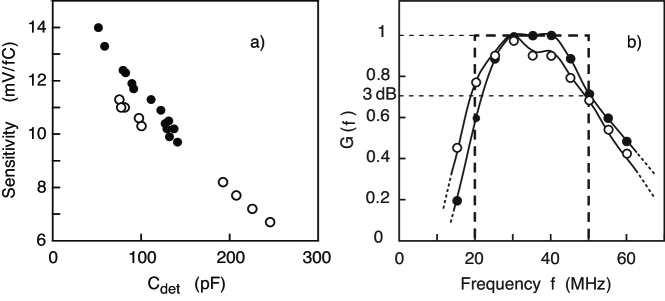
Figure 1: a): Measured sensitivity of the amplifier. b): Measured gain $G$ of the amplifer for a sinusoidal signal as function of frequency $f$. The curves are normalized to their maximum value. The rectangular approximation to the frequency spectrum of the amplifier gain, as used in the MC simulation, is indicated with the 3dB limits at 20 and 50 MHz. The lines are to guide the eye. In both figures the open (full) points refer to negative (positive) input polarity.

The gain of the amplifier (figure 1b) was measured as function of frequency at $C_{det}\simeq 0$. The 3dB limits were found to lie near 20 and 50MHz, for positive and negative input polarity. The output of each amplifier, which has the same sign for cathode and anode readout, is sent to a discriminator.

2.2 The discriminator

A 8-bit digital-to-analog converter (DAC) with 256 steps allows to change the threshold of each discriminator in steps of 2.35 mV which corresponds to a single DAC register unit ($r.u.$). The threshold can vary from positive to negative values, with the exception of a “bias” interval $V_{b}\simeq\pm 26$ mV (figure 2) around zero. In this region the transition between positive and negative threshold occurs within one DAC register. The amplitude of the signal at the input of the amplifier depends on the capacitance of the pad read by the front-end.

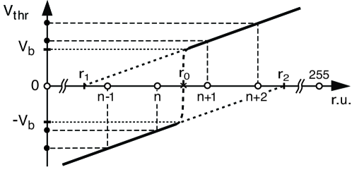
Figure 2: Dependence of the threshold ($V_{thr}$) of the CARIOCA discriminator around zero on the DAC register units ($r.u.$).

For an ideal discriminator with no bias interval, the dependence of the noise counting rate on the threshold is a bell-shaped distribution (figure 3a). Two parameters of this distribution will be considered in the following: the counting rate at zero threshold ($R_{0}$) and the r.m.s. ($\sigma_{R}$) of the distribution.

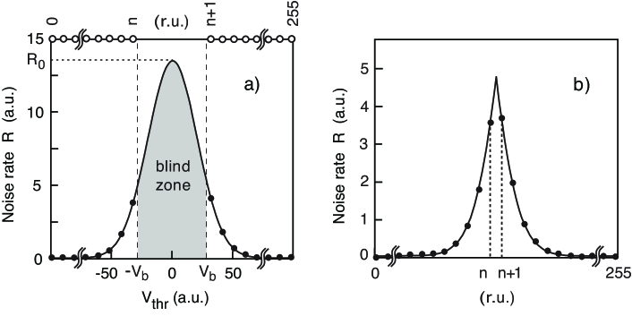
Figure 3: a): Noise counting rate of an ideal discriminator as a function of its threshold (continuous curve). With the CARIOCA discriminator the threshold values comprised in the shaded area cannot be set and the rate at zero threshold ($R_{0}$) cannot be measured. In the upper scale the DAC registers which set the thresholds are schematically reported. b): Typical experimental curve representing the noise counting rate of a CARIOCA discriminator as a function of the DAC registers.

For the CARIOCA discriminator, because of its bias interval, only the tails of the bell-shaped distribution can be measured. A threshold scan will therefore result in a double-arm curve with a cusp (figure 3b), the right (left) arm corresponding to the positive (negative) tails.

To monitor the MWPC readout channels a check of the stability of the $\sigma_{R}$ values of all the 122k channels is periodically performed. For each channel, $\sigma_{R}$ must be inferred from the corresponding threshold scan distribution. This evaluation would be more precise if the shape of the distribution were known. To find out this distribution in the present experimental situation, a Monte Carlo (MC) simulation was performed.

3 The Monte Carlo simulation

The MC simulation comprises the generation of the noise signal sent to the discriminator by the amplifier and the calculation of the output rate of the discriminator as a function of its threshold. The effect of the dead time of the CARIOCA was evaluated. The bias interval was not considered in the MC but will be taken into account later.

3.1 The noise signal

The noise at the input of the front-end electronics is assumed to have a flat frequency spectrum (white noise), resulting from the superposition of a great number of contributions which occur randomly. This noise is then filtered by the amplifier and sent to the discriminator. Therefore the passband of the amplifier determines the frequency spectrum of the noise at the discriminator input. In the MC this passband was approximated to a rectangular one, extending from 20 MHz to 50 MHz, which corresponds to the 3 dB bandwith of the amplifier (figure 1b). This approximation will allow to compare easily the MC results with Rice’s theory [9], and is expected to give a satisfactory representation of the experimental situation.

The time dependence of the noise signal $V(t)$ at the input of the discriminator was generated as a superposition of $N=60000$ sinusoids according to the formula:

$$V(t)=A\sum\limits_{k=1}^{N}sin(2\pi f_{k}t+\phi_{k})$$ (1)

The frequency $f_{k}$ and the phase $\phi_{k}$ were randomly extracted in the intervals $20-50$ MHz and $0-2\pi$ respectively. The noise signal was calculated every 3 ns, assuming $A=1$ in equation 1. With an upper frequency of $\sim 50$ MHz this sampling of the noise is sufficiently dense to give a correct description of the signal.

 

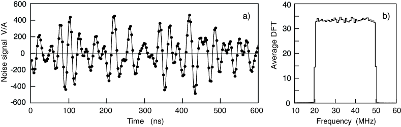
Figure 4: a): A typical simulated noise signal. The points are the values calculated every 3 ns. b): Discrete Fourier transform of 10⁶ consecutive noise values, corresponding to a time interval of 3 ms. The DFT values have been averaged on 0.7 MHz bins.

The MC generates $2\times 10^{8}$ consecutive values of the noise signal, corresponding to a time interval of 600 ms. As shown in the next section, this time interval gives a number of threshold crossings sufficiently high to simulate with good statistics the tails of the threshold scan distribution. In figure 4a we report a small part of the simulated noise signal.

To check the accuracy of the noise simulation a discrete Fourier transform (DFT) of $10^{6}$ consecutive noise values (corresponding to a 3 ms time interval) was performed. The results, shown in figure 4b, reproduce quite well the bandwidth assumed in the MC, giving confidence in the signal generation procedure.

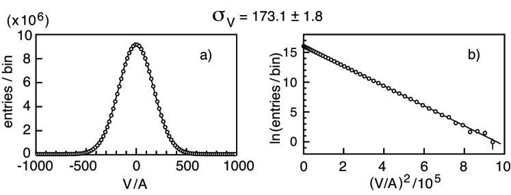
Figure 5: a): Distribution of the $2\times 10^{8}$ values of the noise amplitude $V/A$ (equation 1). In figure b) the same distribution is reported with logarithmic-quadratic scales.

The distribution of the noise amplitudes, calculated with equation 1 every 3 ns, is reported in figure 5a. The r.m.s. of this distribution, deduced from a Gaussian fit, is $\sigma_{V}=173.1\pm 1.8$. The same points, reported in figure 5b with logarithmic-quadratic scales, appear to be perfectly aligned up to $(V/A)^{2}\simeq 9\times 10^{5}$. This confirms that the distribution of the noise amplitudes is, with an excellent approximation, a Gaussian up to $\sim 6\sigma$. As a further check $\sigma_{V}$ was also calculated from the series of generated values of $V(t)$, according to the formula:

$$\sigma_{V}=\left\{\overline{(V(t)/A)^{2}}\right\}^{1/2}=\left\{\overline{\left[\sum\limits_{k=1}^{N}sin(2\pi f_{k}t+\phi_{k})\right]^{2}}\right\}^{1/2}=\sqrt{N/2}=173.2\vspace*{7truemm}$$ (2)

a value in quite good agreement with the one obtained with the Gaussian fit.

The quantity $\sigma_{V}$ is related to the equivalent noise charge (ENC) which is defined as the $\delta$-like charge sent to the front-end which delivers an output signal equal to $\sigma_{V}$.

3.2 The discriminator counting rate

To identify the threshold crossings, a continuous noise signal was necessary. This was obtained by a linear interpolation between consecutive pairs of MC generated points. The discriminator was considered to fire when this signal crosses the threshold with positive (negative) slope for positive (negative) thresholds. The counting rate ($R$) of the discriminator was then determined as a function of its threshold. The result is reported in figure 6a. The same points, reported in figure 6b with logarithmic-quadratic scales, are perfectly aligned up to $(V_{thr}/A)^{2}\simeq 9\times 10^{5}$. This confirms [9, 10, 11] that the distribution of the noise counting rate (figure 6a) is, with an excellent approximation, a Gaussian up to $\sim 6\sigma$. A Gaussian fit to this distribution gives an r.m.s. value $\sigma_{R}=170.3\pm 1.5$.

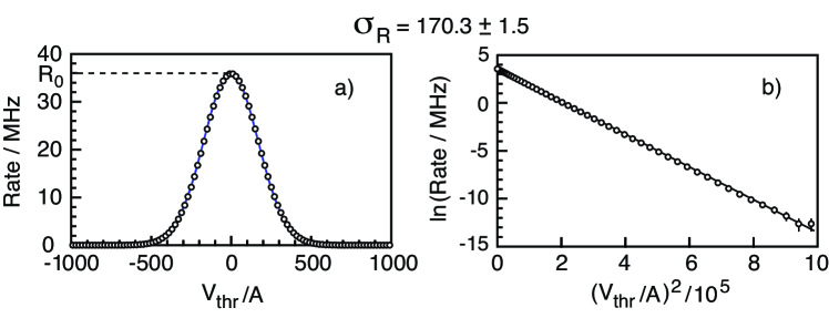
Figure 6: a) Counting rate of the discriminator as a function of its threshold. b) Same as in a) but presented with logarithmic-quadratic scales.

Within the errors, the MC results shown in figure 5 and figure 6 confirm the relation predicted by Rice [9]:

$$\sigma_{V}=\sigma_{R}\equiv\sigma$$ (3)

which links the r.m.s. of two a priori different distributions, and allows to evaluate $\sigma_{V}$ and therefore the ENC of a channel, by measuring its noise rate as a function of the discriminator threshold.

With an ideal discriminator without any bias interval, the counting rate would depend on $V_{thr}$ (figure 6a) according to the formula:

$$R=R_{0}\;\mathrm{exp}\;[-V_{thr}^{2}/(2\sigma^{2})]$$ (4)

The counting rate ($R_{0}$) at zero threshold, calculated from a fit to the MC results (figure 6), is $35.7\pm 1.7$ MHz, in quite good agreement with the value calculated with the Rice formula for a flat bandwidth:

$$R_{0}=\left[\frac{f_{b}^{3}-f_{a}^{3}}{3(f_{b}-f_{a})}\right]^{1/2}=36.1\;\mathrm{MHz}$$ (5)

where $f_{a}=20$ MHz and $f_{b}=50$ MHz are the lower and upper cut-off frequencies of the bandwidth.

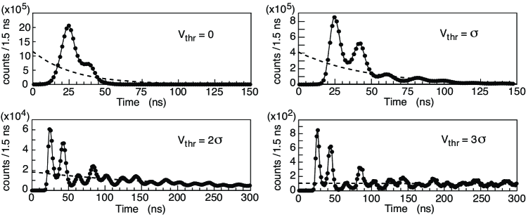
Figure 7: Monte Carlo predictions for the distribution of the time intervals between two consecutive threshold crossing, for four different threshold values. The dashed curves represent the same distributions if the crossing times were completely uncorrelated.

If the exact passband $G(f)$ (figure 1b) of the front-end amplifier is considered, the rate at zero threshold may be calculated numerically from the general Rice formula [9]:

$$R_{0}=\left[\frac{\int\limits_{0}^{\infty}\;f^{2}\>W(f)\;\mathrm{d}f}{\int\limits_{0}^{\infty}\;W(f)\;\mathrm{d}f}\right]^{1/2}=\left[\frac{\int\limits_{0}^{\infty}\;f^{2}\>G^{2}(f)\;\mathrm{d}f}{\int\limits_{0}^{\infty}\;G^{2}(f)\;\mathrm{d}f}\right]^{1/2}$$ (6)

where $W(f)$ is the power spectrum of the noise at the input of the discriminator and $W(f)\propto G^{2}(f)$ for white noise. From equation 6 it turns out to be $R_{0}\simeq 38\pm 3$ MHz for negative polarity and of $R_{0}\simeq 40\pm 3$ MHz for positive polarity, the error being due to non-perfect knowledge of $G(f)$.

At low threshold, and therefore at high counting rate, the effect of the dead time of the CARIOCA ($\sim 55$ ns for noise signal) must be considered. To evaluate this effect, the distribution of the time intervals between two consecutive threshold crossings was calculated with the MC. In figure 7 this distribution is reported for four threshold values. At the lowest thresholds reached in the threshold scans (about 2$-$2.5$\sigma$, see section 4.1) the loss in couting rate due to the dead time is about 15$-$20 %. This effect corresponds to a variation < 2 % on $\sigma$ and was therefore neglected.

4 Experimental results

4.1 Threshold determination

The threshold scan of all the readout channels is performed regularly between two data taking periods. For each channel and for each threshold the noise is counted during 200 ms.

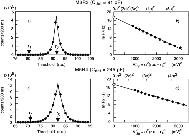
Figure 8: a): Experimental threshold scan of a readout channel of region M3R3. In b) the right-arm of this distribution is represented with logarithmac-quadratics scales. The open point at zero threshold is the counting rate predicted by Rice theory and by the MC. The straight line is the best fit to the points (see text). c) and d): same as a) and b) for a readout channel belonging to region M5R4. The larger detector capacitance ($C_{det}$) results in a larger $\sigma$.

As an example, two threshold scans are shown in figure 8a and 8c, one for a readout channel belonging to region M3R3 (with a cathode readout and a pad capacitance of $\sim 91$ pF) and the other to M5R4 (with an anode readout and a capacitance of $\sim 245$ pF). The two arms of the experimental distributions being almost symmetrical, only the right-arms are considered in the following.

Taking into account the characteristics of the CARIOCA discriminator, the bias interval ($V_{b}$) and the threshold ($V_{thr}$) depend on the DAC register (figure 2) according to the relations:

$$V_{b}= \alpha\>(r_{0}-r_{1})$$ (7)

$$V_{thr}= \alpha\>(r.u.-r_{1})\qquad(r.u.>r_{0})$$ (8)

where $\alpha=2.35$ mV/$r.u.$, $r_{0}$ is the interpolated DAC register corresponding to the threshold jump from positive to negative values and $r_{1}$ is the interpolated register corresponding to the zero threshold for the right arm of the threshold scan (figure 2). The experimental data, were represented on the plane ($\;(r.u.-r_{1})^{2}\;,\;\mathrm{ln}\;R\;$) and fitted to a straight line given by the equation:

$$\mathrm{ln}\;R=\mathrm{ln}\;R\,^{\prime}_{0}-\alpha^{2}(r.u.-r_{1})^{2}/(2\,\sigma^{2})\vspace*{7truemm}$$ (9)

where ln$\;R\,^{\prime}_{0}$ and $\sigma^{2}$ are the parameters of the fit. The value of $r_{1}$ being a priori not known, the fit was repeated for different values of $r_{1}$ until the value of $\;\mathrm{ln}\;R\,^{\prime}_{0}$ obtained from the fit is as close as possible to the expected value of ln$\;R_{0}$, where $R_{0}$ is given by equation 6.

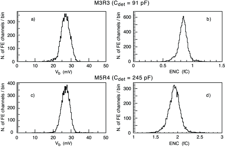
Figure 9: Distribution of: a) the bias voltage; b) the ENC measured for of all the reaudout channels of the region M3R3. c) and d): same as a) and b) for the readout channels belonging to region M5R4.

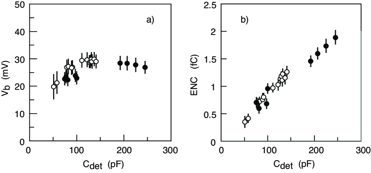
Figure 10: Dependence: a) of the bias voltage ($V_{b}$) and b) of the ENC, on the detector capacitance. Open (full) points refer to cathode (anode) readout. The error bars represent the r.m.s. of the distributions.

It is worthwhile to note that in equation 9, $\sigma$ is related to $R\,^{\prime}_{0}$ through its logarithm. Therefore the effect of the detector capacitance on the noise spectrum and therefore on $R\,^{\prime}_{0}$ has no significant consequence on the value of $\sigma$.

In figure 8b and 8d the experimental points belonging to the right-arms of the threshold scans are reported with logarithmic-quadratic scales together with the results of the fitting procedure. The agreement is quite good up to $\sim 5\,\sigma$.

From equation 9 it turns out that the slope of the fitting line is inversely proportional to $\sigma^{2}\;$ i.e. to $\mathrm{ENC}^{2}$, For the two readout channels considered in figure 8 the results of the fits were for M3R3: $\sigma=4.36$ $r.u.$ $=10.2$ mV; $r_{0}=91.4$ $r.u.$; $r_{1}=80.3$ $r.u.$ and for M5R4: $\sigma=5.56$ $r.u.$ $=13.1$ mV; $r_{0}=82.0$ $r.u.$; $r_{1}=70.8$ $r.u.$ Taking into account the detector capacitance and the corresponding sensitivity (figure 1a and Table 1), the values of $\sigma$ correspond to an ENC = 0.80 fC for M3R3 and 1.89 fC for M5R4. In figure 9 the distribution of the bias voltage $V_{b}$ and of the ENC are reported for all the channels of the regions M3R3 and M5R4.

In figure 10 the mean value of the bias ($V_{b}$) and of the ENC is reported as a function of the pad capacitance of all the different chamber types of the muon detector. As expected, $V_{b}$ is characteristic of the discriminator and is roughly independent of $C_{det}$, while the increase of ENC with $C_{det}$ is approximately linear [13].

A summary of the measured characteristics of the readout channels of different regions is reported in Table 1. The measured ENC values allow to set the working condition of each type of muon chamber for the LHCb data taking. In fact the thresholds should be sufficiently high to limit the counting rate due to electronic noise and sufficiently low to ensure the best time resolution and the maximum detection efficiency of the chambers. Taking into account all these conditions the thresholds were adjusted around 5$-$6 ENC for all chambers.

Table 1: Characteristics of the readout channels of the different regions. The average and the r.m.s. of the ENC and of the bias experimental distributions are reported in the last 4 columns.

		$C_{det}$	Sensitivity	$\overline{\mathrm{ENC}}$	r.m.s. ENC	$\overline{\mathrm{Bias}}$	r.m.s. Bias
Region	Readout	(pF)	(mV/fC)	(fC)	(fC)	(mV)	(mV)
M1R2	cathode	58	13.3	0.41	0.08	21.1	3.9
M1R3	cathode	51	14.0	0.35	0.09	19.7	4.3
M1R4	anode	100	10.3	0.96	0.25	23.0	2.2
M2R1	cathode	131	10.5	1.13	0.11	29.6	2.4
M2R1	anode	75	11.3	0.71	0.12	22.6	3.1
M2R2	cathode	111	11.3	0.97	0.09	29.3	2.5
M2R2	anode	77	11.0	0.70	0.10	23.3	2.7
M2R3	cathode	89	11.9	0.76	0.09	26.6	2.5
M2R4	anode	192	8.2	1.46	0.12	28.4	2.5
M3R1	cathode	137	10.2	1.16	0.13	29.7	2.5
M3R1	anode	81	11.0	0.60	0.07	22.3	2.9
M3R2	cathode	122	10.9	1.03	0.11	29.5	2.6
M3R2	anode	97	10.6	0.68	0.08	23.8	2.6
M3R3	cathode	91	11.7	0.80	0.09	26.8	2.4
M3R4	anode	207	7.7	1.60	0.12	28.3	2.5
M4R1	cathode	79	12.4	0.69	0.09	26.9	2.6
M4R2	cathode	127	10.4	1.12	0.10	28.5	2.4
M4R3	cathode	129	10.2	1.17	0.09	28.9	2.4
M4R4	anode	225	7.2	1.74	0.13	27.7	2.5
M5R1	cathode	82	12.3	0.72	0.09	27.1	2.7
M5R2	cathode	132	9.9	1.22	0.10	28.8	2.4
M5R3	cathode	141	9.7	1.27	0.11	28.9	2.3
M5R4	anode	245	6.7	1.89	0.13	26.9	2.2

4.2 Malfunctionning channels and ageing effects

The method described allows to detect breakdown of some front-end or any possible ageing effects, by checking the stability of the ENC for all the readout channels. In figure 11a the ENC measured in the year 2012 is compared with that measured in 2009. Most of the channels are stable, and only few tens, out of 122k, show a significant change of their ENC value and need to be individually checked, repaired or replaced. In particular a series of channels (indicated by an arrow in figure 11a) appear to be aligned out of the scatter plot bisector which suggests a possible failure in the correct threshold setting by the DACs. Most of these channels belonged to the same boards, which were replaced. The distribution of the difference between the ENC measured in the years 2009 and 2012 is reported in figure 11b. The large peak around zero shows that most of the frontends are quite stable over many years and no ageing effects were observed up to 2 fb^-1, which corresponds to about one tenth of the total integrated luminosity expected in 10 years operation.

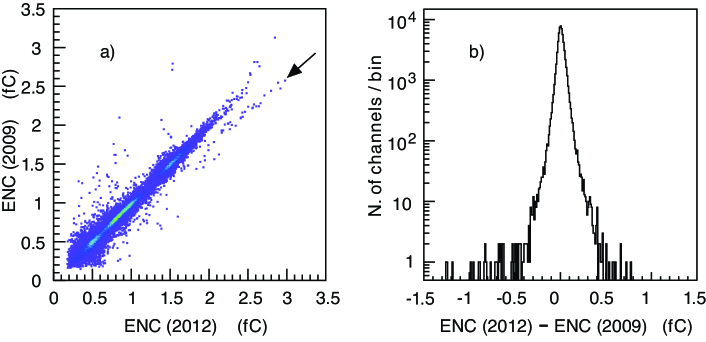
Figure 11: a): Scatter plot of the ENC values measured on all the muon detector in the years 2009 and 2012. The channels which are far from the plot bisector were checked and repaired or replaced. Most of the points in the series indicated by an arrow correspond to CARIOCAs mounted on the same boards which were replaced. b): Distribution of the difference between the ENC measured in 2012 and 2009.

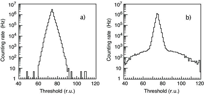
Figure 12: Experimental threshold scanning for: a) a properly behaving front-end channel; b) a malfunctioning channel with an abnormal noise.

Another signal of malfunctioning of a channel readout is an abnormal shape of the threshold scan. A typical example in shown in figure 12.

5 Conclusions

A new method has been introduced which allows to monitor the correct operation of the front-end channels of the LHCb muon detector and to set the optimal discriminator thresholds. The method consists in measuring the noise rate as a function of the discriminator thresholds. The resulting threshold scan distribution is fitted to a tail of a Gaussian as suggested by Rice theory and confirmed by a Monte Carlo simulation. The fitting procedure is greatly facilitated by the knowledge of the counting rate at zero threshold, which cannot be measured but can be calculated from the amplifier bandwidth using the Rice’s formulas. For each threshold scan of a readout channel, the r.m.s. of the fitted Gaussian tail turns out to be equal to the equivalent noise charge (ENC) of that channel. The measurement of the ENC of all the channels allows to check for a possible malfunction or breakdown and to set the working values of the thresholds which satisfy the requirements of a low counting rate due to electronic noise and a high detection efficiency and time resolution of the chambers.

References

- [1] A. Augusto Alves Jr. et al., The LHCb Detector at the LHC, \jinst32008S08005.
- [2] A. Augusto Alves Jr. et al., Performance of the LHCb muon system, arXiv:1211.1346, submitted to JINST.
- [3] W.Bonivento et al., Development of the CARIOCA front-end chip for the LHCb muon detector, Nucl. Instrum. Meth. A 491 (2002) 233.
- [4] E. Dané, et al., Detailed study of the gain of the MWPCs for the LHCb muon system, Nucl. Instrum. Meth. A 572 (2007) 682.
- [5] L. Gruber, W.Riegler and B.Schmidt, Time resolution limits of the MWPCs for the LHCb muon system, Nucl. Instrum. Meth. A 632 (2011) 69.
- [6] A. P. Kashchuk and O. V. Levitskaya, From noise to signal- a new approach to LHCb muon optimization, LHCb note, LHCb-PUB-2009-018 (2009), (http://cdsweb.cern.ch/record/1209624/files/LHCb-PUB-2009-018.pdf) and references therein quoted.
- [7] A. P. Kashchuk, Application of the Rice theory for reconstructing the noise distributions in nuclear electronics, Instruments and Experimental Techniques 55 (2012) 440, engl. transl. of Pribory i Tekhnika Eksperimenta 4 (2012) 26.
- [8] L. Gruber, Optimization of the operating parameters of the LHCb muon system, CERN-THESIS-2010-037 (2010).
- [9] S. O. Rice, Mathematical analysis of random noise, Bell System Technical Journal 23 (1944) 282 and 24 (1945) 46.
- [10] M. Kac, On the Distribution of Values of Trigonometric Sums with Linearly Independent Frequencies, Amer. Jour. Math. 65 (1943) 609.
- [11] V. A. Ivanov, On the Average Number of Crosssings of a Level by Sample Functions of a Stochastic Process, Theory of Probability and Its Applications, engl. transl. of Teor. Veroyatnost. i Primen. 5 (1960) 319.
- [12] M. S. Longuet-Higgins, The Distribution of Intervals between Zeros of a Stationary Random Function, Phil. Trans. Royal Society of London; Series A, Math. and Phys. Sciences 254 (1962) 557 (http://www.jstor.org/stable/73149), and references therein quoted.
- [13] F. Anghinolfi, Front-end Electronics, Course on Detectors and Electronics for High Energy Physics, Astrophysics and Space Applications, INFN Laboratori Nazionali di Legnaro, 26-30 March 2007.