Improving predictive power of physically based rainfall-induced shallow landslide models: a probabilistic approach

Zusammenfassung

Distributed models to forecast the spatial and temporal occurrence of rainfall-induced shallow landslides are based on deterministic laws. These models extend spatially the static stability models adopted in geotechnical engineering, and adopt an infinite-slope geometry to balance the resisting and the driving forces acting on the sliding mass. An infiltration model is used to determine how rainfall changes pore-water conditions, modulating the local stability/instability conditions. A problem with the operation of the existing models lays in the difficulty in obtaining accurate values for the several variables that describe the material properties of the slopes. The problem is particularly severe when the models are applied over large areas, for which sufficient information on the geotechnical and hydrological conditions of the slopes is not generally available. To help solve the problem, we propose a probabilistic Monte Carlo approach to the distributed modeling of rainfall-induced shallow landslides. For the purpose, we have modified the Transient Rainfall Infiltration and Grid-Based Regional Slope-Stability Analysis (TRIGRS) code. The new code (TRIGRS-P) adopts a probabilistic approach to compute, on a cell-by-cell basis, transient pore-pressure changes and related changes in the factor of safety due to rainfall infiltration. Infiltration is modeled using analytical solutions of partial differential equations describing one-dimensional vertical flow in isotropic, homogeneous materials. Both saturated and unsaturated soil conditions can be considered. TRIGRS-P copes with the natural variability inherent to the mechanical and hydrological properties of the slope materials by allowing values of the TRIGRS model input parameters to be sampled randomly from a given probability distribution. The range of variation and the mean value of the parameters can be determined by the usual methods used for preparing the TRIGRS input parameters. The outputs of several model runs obtained varying the input parameters are analyzed statistically, and compared to the original (deterministic) model output. The comparison suggests an improvement of the predictive power of the model of about 10 % and 16 % in two small test areas i.e., i.e., the Frontignano (Italy) and the Mukilteo (USA) areas. We discuss the computational requirements of TRIGRS-P to determine the potential use of the numerical model to forecast the spatial and temporal occurrence of rainfall-induced shallow landslides in very large areas, extending for several hundreds or thousands of square kilometers. Parallel execution of the code using a simple process distribution and the Message Passing Interface (MPI) on multi-processor machines was successful, opening the possibly of testing the use of TRIGRS-P for the operational forecasting of rainfall-induced shallow landslides over large regions.

Rainfall is a primary trigger of landslides, and rainfall-induced landslides are common in many physiographical environments, e.g. Brabb and Harrod (1989). Prediction of the location and time of occurrence of shallow rainfall-induced landslides remains a difficult task, which can be accomplished adopting empirical (Crosta, 1998; Sirangelo et al., 2003; Aleotti, 2004; Guzzetti et al., 2007, 2008), statistical (Soeters and Van Westen, 1996; Guzzetti et al., 1999, 2005, 2006a; Committee on the Review of the National Landslide Hazards Mitigation Strategy, 2004), or process based (Montgomery and Dietrich, 1994; Terlien, 1998; Baum et al., 2002, 2008, 2010; Crosta and Frattini, 2003; Simoni et al., 2008; Godt et al., 2008; Vieira et al., 2010) approaches, or a combination of them (Gorsevski et al., 2006; Frattini et al., 2009). Inspection of the literature, reveals that process based (deterministic, physically based) models are preferred to forecast the spatial and the temporal occurrence of shallow landslides triggered by individual rainfall events in a given area. Process based models rely upon the understanding of the physical laws controlling slope instability. Due to lack of information and the poor understanding of the physical laws controlling landslide initiation, only simplified, conceptual models are possible, currently. These models extend spatially the simplified stability models widely adopted in geotechnical engineering e.g., Taylor (1948); Wu and Sidle (1995); Wyllie and Mah (2004), and calculate the stability / instability of a slope using parameters such as normal stress, angle of internal friction, cohesion, pore-water pressure, root strength, seismic acceleration, external weights. Computation results in the factor of safety, an index expressing the ratio between the local resisting ($R$) and driving ($S$) forces, $F_{\mathrm{S}}=R/S$. Values of the index smaller than 1, corresponding to $R<S$, denotes instability, on a cell-by-cell basis, according to the adopted model. To calculate the resisting and the driving forces, the geometry of the sliding mass must be defined, including the geometry of the topographic surface and the location of the slip surface. Most commonly, an infinite-slope approximation is adopted (Taylor, 1948; Wu and Sidle, 1995). This is also the approach adopted by the US Geological Survey (USGS) Transient Rainfall Induced and Grid-Based Regional Slope-Stability Model (TRIGRS) model (Baum et al., 2002, 2008), within each user-defined cell. Within the infinite-slope approximation, in each cell the slip surface is assumed to be of infinite extent, planar, at a fixed depth, and parallel to the topographic surface. Forces acting on the sides of the sliding mass are neglected.

Abbildung 1: (A) Example of a rainfall-induced shallow landslide of the soil slide type in the Collazzone area, Umbria, Italy (Figure 7). (B) Schematic representation of the slope-infinite model showing the coordinate system and variables used in the deterministic and probabilistic models. See Table 9 for the symbols description.

Modeling of shallow landslides (Figure 1a) triggered by rainfall adopting the infinite-slope approach requires time-invariant and time-dependent information. Time-invariant information includes the mechanical and hydrological properties of the slope material (e.g. unit weight $\gamma$, cohesion $c$, angle of internal friction $\phi$, water content $\theta$, saturated hydraulic conductivity $K_{\mathrm{s}}$), and the geometrical characteristics of the sliding mass (e.g., gradient of the slope and the sliding plane $\delta$, depth to the sliding plane $d_{\text{fp}}$). The fact that these parameters are constant in time is an assumption of the model. Time-dependent information consists of the pressure head $\psi$, i.e. the pressure exerted by water on the sliding mass, a function of the depth, $d_{\mathrm{w}}$ of water in the terrain (Freeze and Cherry, 1979). Determining the pressure head, and its spatial and temporal variations, requires understanding how rainfall infiltrates and water moves into the ground. This is described by the Richards equation (Richards, 1931). This non-linear partial differential equation does not have a closed-form analytical solution, and approximate solutions are used for saturated (e.g., Iverson, 2000) and unsaturated (e.g,. Srivastava and Yeh, 1991; Savage et al., 2003, 2004) conditions.

The numerical implementation of one such model has been accomplished by Baum et al. (2002) in TRIGRS. The program calculates the stability conditions of individual grid cells in a given area, and models infiltration adopting the approach proposed by Iverson (2000), for one-dimensional vertical flow in isotropic, homogeneous materials, and for saturated conditions. In the code, the forces acting on each individual grid cell are balanced in the centre of mass of each cell, and all interactions with the neighboring grid cells are neglected.

In a second release of TRIGRS, Baum et al. (2008) have extended the code to include unsaturated soil conditions, including the presence of a capillary fringe above the water table. TRIGRS can be used for modeling and forecasting the timing and spatial distribution of shallow, rainfall-induced landslides in a given area (Baum et al., 2002, 2008, 2010). A problem when using TRIGRS, and similar computer codes (e.g. Shalstab, Montgomery and Dietrich, 1994; GEOtop-SF, Simoni et al., 2008), for the modeling of shallow rainfall-induced landslides over large areas resides in the difficulty (or operational impossibility) of obtaining sufficient, spatially distributed information on the mechanical and hydrological properties of the

Abbildung 2: The location of the Mukilteo study area, near Seattle, WA, USA.

terrain. Adoption of a particular value to describe the mechanical (unit weight $\gamma_{\mathrm{s}}$, cohesion $c$, angle of internal friction $\phi$) and the hydrological (water content $\theta$, saturated hydraulic conductivity $K_{\mathrm{s}}$) properties of the terrain may result in unrealistic or inappropriate representations of the stability conditions of individual or multiple grid cells.

In this work, we propose a probabilistic, Monte Carlo approach in an attempt to overcome the problem of poor knowledge of terrain characteristics over large study areas. We obtain the input values for the parameters for the individual runs of TRIGRS using probability distributions. Multiple simulations are performed with different sets of randomly chosen input parameters, and we obtain multiple sets of model outputs.We denote the newly developed code TRIGRS-Probabilistic, or TRIGRS-P. The different outputs are then analysed jointly to infer local stability or instability conditions as a function of the random variability of the input parameters, and the statistical significance of the multiple outputs is determined. Examples of similar probabilistic approaches to model the stability/instability conditions of slopes exists in the literature (e.g., Hammond et al. (1992); Pack et al. (1998); Haneberg (2004)). The various models adopt different physically-based models, which are not equivalent. We maintain that the probabilistic approach of the modified version of TRIGRS is relevant, because it considers most of the aspects relevant to slope stability analysis, and it is capable of reproducing empirical properties of rainfall-induced shallow landslides, including the rainfall intensity-duration conditions that generate the slope instabilities, and the statistics of the size of the unstable areas, as recently shown by Alvioli et al. (2014).

The paper is organized as follows. First, we summarize the model adopted in the software code TRIGRS, version 2.0 (Baum et al., 2008), and we introduce our probabilistic extension (Sect. 1) implemented in the new code TRIGRS-P. Next, we present a comparison of the performance of the original and the probabilistic simulations for two study areas: Mukilteo, USA, and Frontignano, Italy (Sect. 2). Results are discussed in Sect. 3, which focuses on the analysis of the performance of the geographical prediction of the shallow landslides, and on the potential application of the new probabilistic code for modeling shallow rainfall-induced landslides over large areas ($>$ 100 km^2).

1 Overview of the model

Both TRIGRS and TRIGRS-P frameworks are pixel-based and adopt the same geometrical scheme, the same subdivision of the geographical domain and accept the same inputs. An additional set of parameters is used in TRIGRS-P to specify the variability of the characteristics of the terrain. Within each pixel, slopes are modeled as a two-layer system consisting of a lower saturated zone with a capillary fringe above the water table, overlain by an unsaturated zone that extends to the ground surface. The water table and the (hypothetical) sliding surface are planar and parallel to the topographic surface. The geographical domain represented by an array of grid cells, coincides with the elements of a digital elevation model (DEM) used to describe the topography of the study area (Figure 1b).

1.1 Deterministic approach: the TRIGRS code

In the original approach coded in TRIGRS (Baum et al., 2008), the stability of an individual grid cell is determined adopting the one-dimensional infinite-slope model Taylor (1948). The model assumes that failure of a grid cell occurs when the resisting forces $R$ acting on the sliding surface are less than the driving forces $S$ (Wu and Sidle, 1995; Wyllie and Mah, 2004). The ratio of the resisting $R$ and the driving $S$ forces gives by the factor of safety $F_{\mathrm{S}}$,

$$F_{\mathrm{S}}=\frac{R}{S}=\frac{\tan\phi}{\tan\delta}+\frac{c-\psi\,\gamma_{\mathrm{w}}\tan\phi}{\gamma_{\mathrm{s}}z\sin\delta\cos\delta}\,,$$ (1)

where the internal friction angle $\phi$, the cohesion $c$, and the soil unit weight ${\gamma}_{\mathrm{s}}$ describe the material properties, $\gamma_{\mathrm{w}}$ is the groundwater unit weight, $\delta$ is the angle of the planar slope, and $\psi$ is the pressure head (Figure 1b, see Table 9). Failure occurs when $F_{\mathrm{S}}<1$. Solution of Equation (1) requires the

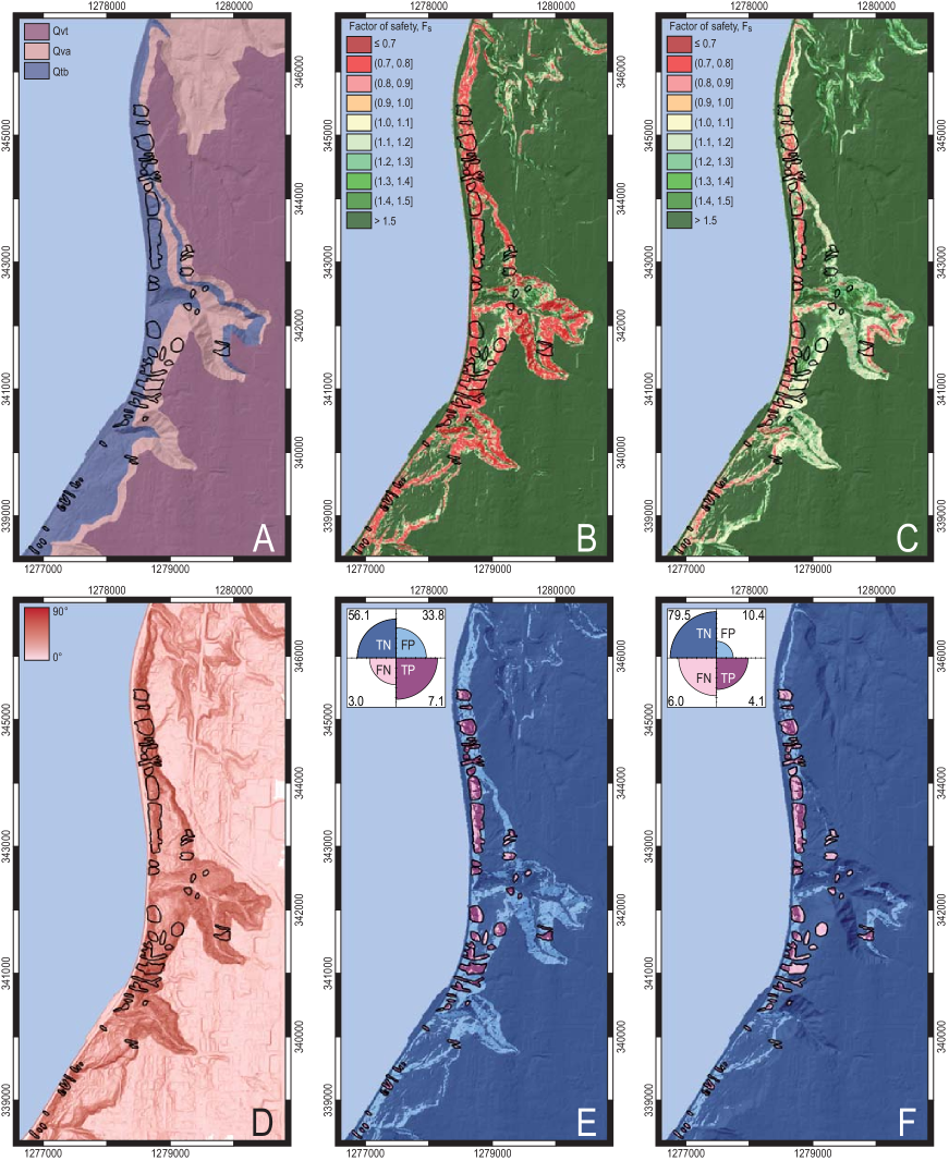
Abbildung 3: Mukilteo study area; results obtained using the original TRIGRS code and input parameters of Table 1. (A) Lithology map: Qtb, transition sediments, including the Lawton Clay ($1$ in Table 1); Qva, Advance outwash sand ($2$ in Table 1); Qvt, Glacial till ($3$ in Table 1). (B) Factor of safety $F_{\mathrm{S}}$ obtained with saturated soil conditions; (C) $F_{\mathrm{S}}$ obtained with unsaturated soil conditions; (D) slope map; (E) map of correct assignments and model errors, within the saturated model; TP, True Positive; TN, True Negative; FP, False Positive; FN, False Negative; (F) as in (E), for the unsaturated model. Black polygons show rainfall-induced landslides.

Abbildung 4: Mukilteo study area. Maps showing factor of safety $F_{\mathrm{S}}$ obtained with the code presented in this work, TRIGRS-P, initialized with the same input parameters used for the same area and TRIGRS code, in Figure 3, and with the following parameters for the random number generation: (A) $\lambda=0.01$, $\nu=1.0$; (B) $\lambda=0.5$, $\nu=1.0$; (C) $\lambda=1.0$, $\nu=1.0$. (D) $\lambda=0.5$, $\nu=0.8$; (E) $\lambda=0.5$, $\nu=0.9$; (F) $\lambda=0.5$, $\nu=1.1$. We performed 16 runs for each set of parameters. Black polygons show rainfall-induced landslides; the insets show the spatial variability of the factor of safety.

Abbildung 5: Maps of correct assignments and model errors in the Mukilteo study area, obtained with the TRIGRS-P code with different sets of random input parameters. (A) $\lambda=0.01$, $\nu=1.0$; (B) $\lambda=0.5$, $\nu=1.0$; (C) $\lambda=1.0$, $\nu=1.0$. (D) $\lambda=0.5$, $\nu=0.8$; (E) $\lambda=0.5$, $\nu=0.9$; (F) $\lambda=0.5$, $\nu=1.1$. TP, True Positive; TN, True Negative; FP, False Positive; FN False Negative. In all maps, black polygons show rainfall-induced landslides in the study area.

computation of the pressure head $\psi$, which is governed by the Richards (1931) equation:

$$\frac{\partial}{\partial z}\left[K_{z}\left(\psi\right)\frac{\partial\left(\psi-z\right)}{\partial z}\right]=\frac{\partial\theta}{\partial t}\,,$$ (2)

where, $z$ is the slope-normal coordinate, $t$ is the time, $K_{z}$ is the vertical hydraulic conductivity that depends on the pressure head $\psi$, and $\theta$ is the volumetric water content (Figure 1b). Equation (2) is solved in TRIGRS adopting the modeling scheme proposed by Baum et al. (2008).

For saturated conditions, TRIGRS uses a modified version of the analytical solutions of Equation (2) proposed by Iverson (2000), for short term and for long-term rainfall periods. Again, the modification consists chiefly in the possibility of using a complex rainfall history (Baum et al., 2008). To linearize Equation (2), Iverson (2000) adopted a normalization criterion using a length scale ratio as follows:

$$\varepsilon=\sqrt{\frac{d^{2}_{\text{fp}}/D_{0}}{A/D_{0}}}=\frac{d_{\text{fp}}}{\sqrt{A}},$$ (3)

where $D_{0}$ is the maximum hydraulic diffusivity, $A$ is the contributing area that affects hydraulic pressure at the potential failure plane depth $d_{\text{fp}}$, and $d^{2}_{\text{fp}}/D_{0}$ and $A/D_{0}$ are the minimum time required for slope-normal ($d^{2}_{\text{fp}}/D_{0}$) and for slope-lateral ($A/D_{0}$) pore pressure transmission (see Table 9). Under the condition $\varepsilon\ll 1$, simplification of Equation (2) gives (Iverson, 2000):

$$\frac{\partial}{\partial z^{*}}\left[K^{*}(\psi)\left(\frac{\partial\psi^{*}}{\partial z^{*}}-z^{*}\right)\right]=0\,,\,\,\,{\text{for}}\,\,\,t>\frac{A}{D_{0}}$$ (4)

and

$$\frac{\partial}{\partial z^{*}}\left[K^{*}\left(\frac{\partial\psi*}{\partial z^{*}}-z^{*}\right)\right]=\frac{C(\psi)}{C_{0}}\frac{\partial\psi*}{\partial t^{*}}\,,\,\,\,{\text{for}}\,\,\,t\ll\frac{A}{D_{0}},$$ (5)

where $\psi^{*}=\psi/d_{\text{fp}}$, $t^{*}=tD/A\leavevmode\nobreak\$, and $z^{*}=z/\sqrt{d_{\text{fp}}}$.

For unsaturated conditions, the code uses a modified version of the analytical solution of Equation (2) proposed by Srivastava and Yeh (1991), for the case of one-dimensional, transient, vertical infiltration. The modification consists in the use of a variable rainfall history (intensity, duration), allowing modeling of complex rainfall patterns (Baum et al., 2008). Equation (2) was linearized in Srivastava and Yeh (1991), who adopted the following exponential model (Gardner, 1958):

$$K_{z}\left(\psi\right)=K_{\mathrm{s}}\,e^{\alpha\widetilde{\psi}}\,;$$ (6)

$$\theta=\theta_{\mathrm{r}}+\left(\theta_{\mathrm{s}}-\theta_{\mathrm{r}}\right)\,e^{\alpha\widetilde{\psi}}\,,$$ (7)

where $K_{\mathrm{s}}$ is the saturated hydraulic conductivity, $\theta_{\mathrm{r}}$ is the residual water content, $\theta_{\mathrm{s}}$ is the saturated water content, and $\widetilde{\psi}=\psi-\psi_{0}$, $\psi_{0}=-1/\alpha$ is a constant, with $\alpha$ the inverse of the vertical height of the capillary fringe above the water table (Savage et al., 2003, 2004). Substitution of Equation (7) into Equation (2) leads to the partial differential equation:

$$\frac{\alpha\left(\theta_{\mathrm{s}}-\theta_{\mathrm{r}}\right)}{K_{\mathrm{s}}}\frac{\partial K}{\partial t}=\frac{\partial^{2}K}{\partial z^{2}}-\alpha\frac{\partial K}{\partial z}\,.$$ (8)

Equation (8) is a linear diffusion equation for which analytical solutions can be obtained using the Laplace, the Fourier, or the Green’s function methods (Kevorkian, 1991), once boundary conditions are specified, e.g.:

$$K(z,0)=I_{ZLT}-\left[I_{ZLT}-K_{\mathrm{s}}e^{\alpha\psi_{0}}\right]e^{-\alpha z}\,;$$ (9)

$$K(0,t)=K_{\mathrm{s}}e^{\alpha{\psi}_{0}}$$ (10)

where $I_{ZLT}$ is the steady surface flux, which can be approximated by the average precipitation rate necessary to maintain the initial conditions in the days to months preceding an event (Baum et al., 2010). When a solution of Equation (8) is obtained, the pore pressure head $\psi$ can be calculated by inversion of Equation (2). Solutions of Equation (8) with the boundary conditions listed in Equation (10) are given in Appendix A1.

TRIGRS implements a simple surface runoff routing scheme to disperse the excess water from the grid cells where rainfall intensity exceeds the local infiltration capacity (Hillel, 1982; Baum et al., 2008).

1.2 Probabilistic approach: the TRIGRS-P code

In our extension of the TRIGRS code, we use the same model and equations as in the original code. The innovation consists of using probability distributions to model the slope material and hydrological properties, i.e. the values of the input parameters. The geometry of the slope ($\delta$) and the position of the sliding plane ($d_{\text{fp}}$) remain unchanged. The model parameters appearing in the equations described in Sect. 1.1 are replaced by functions of random numbers, i.e.:

$$c=c({\xi}_{\mathrm{c}}),\;{\text{cohesion}};$$

$$\phi=\phi({\xi}_{\phi}),\;\mathrm{angle\,\,\,of\,\,\,internal\,\,\,friction};$$

$${\gamma}_{\mathrm{s}}=\gamma({\xi}_{\gamma}),\;\mathrm{soil\,\,\,unit\,\,\,weight};$$

$$D_{0}=D_{0}({\xi}_{D_{0}}),\;\mathrm{hydraulic\,\,\,diffusivity};$$

$$K_{\mathrm{s}}=K_{\mathrm{s}}({\xi}_{K_{\mathrm{s}}}),\;\mathrm{saturated\,\,\,hydraulic\,\,\,conductivity};$$

$${\theta}_{\mathrm{r}}={\theta}_{\mathrm{r}}({\xi}_{\theta_{\mathrm{r}}}),\;\mathrm{residual\,\,\,water\,\,\,content};$$

$${\theta}_{\mathrm{s}}={\theta}_{\mathrm{s}}({\xi}_{\theta_{\mathrm{s}}}),\;\mathrm{saturated\,\,\,water\,\,\,content};$$

$$\alpha=\alpha({\xi}_{\alpha}),\;\mathrm{inverse\,\,\,height\,\,\,of\,\,\,capillary\,\,\,fringe}$$ (11)

where ${\xi}_{i}$ is a random number, with the subscript i used to specify a different parameter, ${\xi}_{\mathrm{c}}$ for cohesion, ${\xi}_{\phi}$ for friction, etc., so that the parameters can be varied independently from each other. Replacing the parameters listed in Equation (11) into Eqs. (1), (2), (4), (5), and (8), we obtain a system of equations that are initialized with a different, randomly chosen set of parameters at each run of TRIGRS-P. The solution of the various scenarios for saturated or unsaturated conditions are performed in the very same way as

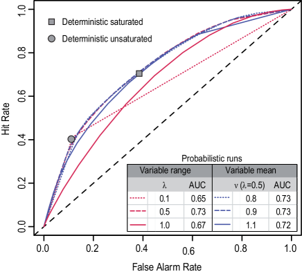
Abbildung 6: The results of simulations for the Mukilteo study area, presented using ROC curves. The grey square and circle represent the results obtained using the original TRIGRS code with saturated and unsaturated initial conditions, respectively (Figure 3b, c); the curves correspond to the results obtained with the TRIGRS-P code, using the variability of input parameters shown in the inset as described in the text (Figures 4 and 5).

in TRIGRS. The depth to the potential sliding plane $d_{\text{fp}}$ was assumed to coincide with the soil depth, and was estimated by Godt et al. (2008) and Baum et al. (2010) using variations of the models proposed by DeRose (1996) and by Salciarini et al. (2006). Additional choices for initial conditions and corresponding sources of uncertainties will be discussed in the following.

We have implemented two probability density functions (pdf) for generating the modeling parameters: (i) the normal distribution function ${\mathcal{N}}$, and (ii) the uniform distribution function ${\mathcal{U}}$. If $\xi$ is a standard normally distributed variable ${\mathcal{N}}{\text{(0,1}}$) with mean $\bar{\xi}=0$ and standard deviation $\sigma=1$, the variable $x=\overline{x}+{\sigma}_{x}\xi$ is normally distributed with mean $\bar{x}$ and standard deviation ${\sigma}_{x}$, ${\mathcal{N}}(\bar{x},{\sigma}_{x})$. Similarly, if $\xi$ is standard uniformly distributed ${\mathcal{U}}(0,1)$, the variable

Tabelle 1: Geotechnical parameters for the geological units cropping out in the Mukilteo area (Figure 3a). $c$, cohesion; $D_{0}$, hydraulic diffusivity; $K_{\mathrm{s}}$, saturated hydraulic conductivity; $\theta_{\mathrm{s}}$, saturated water content; $\theta_{\text{r}}$, residual water content; $\alpha$, inverse of capillary fringe. The friction angle $\phi$ has a common value of 33.6 for the three geological units; units definitions are: 1, Qtb; 2, Qva; 3, Qvt.

Unit	$c$	$D_{0}$	$K_{\mathrm{s}}$	$\theta_{\mathrm{s}}$	$\theta_{\mathrm{r}}$	$\alpha$
	[kPa]	[m2 s-1]	[m s-1]	–	–	[m-1]
1	3.0	$3.8\cdot 10^{-4}$	$1.0\cdot 10^{-4}$	$0.40$	$0.06$	$10$
2	3.0	$5.0\cdot 10^{-6}$	$1.0\cdot 10^{-7}$	$0.40$	$0.10$	$2$
3	8.0	$8.3\cdot 10^{-6}$	$1.0\cdot 10^{-6}$	$0.45$	$0.10$	$5$

Abbildung 7: Map showing location of the Frontignano study area, Umbria, central Italy. The area is located inside the larger Collazzone area (Guzzetti et al., 2006a, b).

$y=y_{a}+(y_{b}-y_{a})\xi$ is uniformly distributed in the range $[y_{a},y_{b}]$, ${\mathcal{U}}(y_{a},y_{b})$. The advantage of using these expansions is that their deterministic limits are obtained for ${\sigma}_{x}\to 0$ and for $\lambda\equiv y_{b}-y_{a}\to 0$, respectively.

In this work, we calculated the stability conditions in the modeling domain for a given set of variables describing the slope materials properties ($\phi$, $c$, ${\gamma}_{\mathrm{s}}$, $K_{\mathrm{s}}$, $D_{0}$, ${\theta}_{\mathrm{r}}$, ${\theta}_{\mathrm{s}}$) obtained by sampling randomly from the uniform distribution only. There is a conceptual difference between the two distributions for distributed landslide probabilistic modeling. Adoption of the Gaussian distribution requires that the investigator has determined (e.g., through sufficient field tests or laboratory experiments) the uncertainty and measuring errors associated with the parameters. The mean and the standard deviation of the Gaussian

Tabelle 2: Estimators of model performance for saturated and unsaturated soil calculated with the original TRIGRS code, for the Mukilteo study area. TPR, True Positive Rate; FPR, False Positive Rate; ACC, Accuracy; PPV, Precision.

Model type	TPR	FPR	ACC	PPV
Saturated	$0.71$	$0.38$	$0.63$	$0.17$
Unsaturated	$0.41$	$0.12$	$0.84$	$0.28$

distribution define unambiguously the uncertainty. Use of the uniform distribution implies that the investigator only knows the possible (or probable) range of variation of the parameters, ignoring the internal structure of the uncertainty. We consider the Gaussian distribution more appropriate to predict rainfall-induced landslides in small areas where sufficient field and laboratory tests were performed to characterize the physical properties of the geological materials, and the uniform distribution best suited in the investigation of large areas where information on the geo-hydrological properties is limited. Further, we consider use of the Gaussian distribution best suited to investigate how errors in the parameters propagate and affect the modeling results, provided that the errors are known. Conversely, use of the uniform distribution allows for investigating how the uncertainty in the model parameters affects the model results. The sensitivity of the extended model to the random variation of model parameters has been explored by running 16 independent simulations, each with a different set of input parameters while keeping unchanged, and equal to the run performed with the original fixed-input TRIGRS model, the terrain morphology ($\delta$) and rainfall history.

2 Deterministic vs. probabilistic approach

We tested the performance of the new probabilistic version of the numerical code, TRIGRS-P $2.0$, against the original TRIGRS code, version 2.0 (Baum et al., 2008), in two study areas. The first test was conducted in the Mukilteo study area, near Seattle, WA, USA (Figure 2). This is the same geographical area where Godt et al. (2008) and Baum et al. (2010) demonstrated the use of TRIGRS in a broad geographical setting. The second test was performed in the Frontignano study area, Perugia, Italy (Figure 7). This is part of the Collazzone geographical area where Guzzetti et al. (2006a, b) have investigated the hazard posed by shallow landslides using multivariate classification methods.

2.1 Mukilteo study area

The three square kilometre study area is located along the eastern side of the Puget Sound, about $15\,\unit{km}$ north of Seattle, WA, USA (Figure 2). In this area, rainfall is the primary trigger of landslides. Slope failures are typically shallow (less than three meters thick), and involve the sandy colluvium and the weathered glacial deposits mantling the coastal bluffs (Galster and Laprade, 1991; Baum et al., 2000). The climate of the Seattle area is characterized by a pronounced seasonal precipitation regime with a winter maximum, and $3/4$ of the annual precipitation falling from November to April (Church, 1974). Storms that trigger shallow landslides in Seattle are generally of long duration (more than 24 h) and of moderate intensity (Godt et al., 2006). Three geological units crop out in the area (Minard, 2000) (Figure 3a) including, from older to younger: (i) transition sediments, comprising the Lawton Clay (Qtb), (ii) advance outwash sand (Qva), and (iii) glacial till (Qvt). The mechanical and hydrological properties of the materials in the three geological units are known through field tests and laboratory experiments (Lu et al., 2006; Godt et al., 2006, 2008), and are summarized in Table 1.

2.1.1 Predictions with the deterministic approach

For modeling purposes, the topography of the area was described by a $6\,\unit{ft}\times 6\,\unit{ft}$ ($1.83\,\unit{m}\times 1.83\,\unit{m}$) DEM obtained through airborne laser-swath mapping (Haugerud et al., 2003). Initial conditions for infiltration were prescribed as zero pressure head at the depth of the lower boundary of colluvium. This is in agreement with field observations (Baum et al., 2005; Schulz, 2007; Godt et al., 2008). A constant rainfall intensity $I=4.5\,\unit{mm\,h^{-1}}$ for a period of 28 h was used to force slope instability, for a cumulative event rainfall $E=126\,\unit{mm}$. The adopted rainfall history represents a limit case of the rainfall intensity-duration conditions that have resulted in landslides in the Mukilteo area in the winter 1996–1997 (Godt et al., 2008; Baum et al., 2010). Figure 3 shows the results of the runs with deterministic input, for saturated (Equation 4, Figure 3b) and for unsaturated (Equation 5, Figure 3c) conditions. For the mechanical and hydrological properties of the geological materials ($\phi$, $c$, ${\gamma}_{\mathrm{s}}$, $K_{\mathrm{s}}$, $D_{0}$, ${\theta}_{\mathrm{r}}$, ${\theta}_{\mathrm{s}}$) we considered the values listed in Table 1.

In order to test the model prediction skills i.e., the ability of the model to forecast the known distribution of rainfall-induced landslides (Guzzetti et al., 2006a), the two geographical distributions of the factor of safety $F_{\mathrm{S}}$ were compared to a landslide inventory showing slope failures triggered by rainfall in the winter 1996–1997 (Baum et al., 2000; Godt et al., 2008), displayed by black lines in Figure 3. For the comparison, all grid cells with $F_{\mathrm{S}}<1$ were considered unstable (i.e., potential landslide) cells. Four-fold plots and maps showing the geographical distribution of the correct assignments and the model errors (Figure 3e, f) are used to summarize and display the comparison. Four-fold plots are graphical representations of contingency tables (or confusion matrices), and show the fraction (or number) of true positives (TP), true negatives (TN), false positives (FP), and false negatives (FN) (Fawcett, 2006; Rossi et al., 2010). In our analysis TP is the percentage of cells with observed landslides, which are predicted as unstable by the model; similarly, TN is the percentage of cells without landslides predicted as stable by the model. Correspondingly, FP (FN) are the percentage of predicted unstable (stable) cells without (with) observed landslides. We will refer to both TP and TN as correct assignment in the following, while FP and FN are model errors. To further quantify the performance of the deterministic forecasts, different metrics were computed (Table 2),

Abbildung 8: As in Figure 3, but for the Frontignano study area. The results have been obtained using the original TRIGRS code with input parameters listed in Table 5. (A) Lithological map: sand ($1$ in Table 5); clay ($2$ in Table 5); flysch deposits ($3$ in Table 5); gravel, sand, silt, and clay ($4$ in Table 5); sand, silt, and clay ($5$ in Table 5). (B) Factor of safety $F_{\mathrm{S}}$ obtained with saturated soil conditions; (C) $F_{\mathrm{S}}$ obtained with unsaturated soil conditions; (D) slope map; (E) map of correct assignments and model errors, within the saturated model; TP, True Positive; TN, True Negative; FP, False Positive; FN, False Negative; (F) as in (E), for the unsaturated model. Black polygons show rainfall-induced landslides.

Abbildung 9: Frontignano study area. Maps of the factor of safety $F_{\mathrm{S}}$ obtained within the probabilistic approach of TRIGRS-P, with the following values of range of variation of input parameters: (A) $\lambda=0.01$, $\nu=1.0$; (B) $\lambda=0.75$, $\nu=1.0$; (C) $\lambda=1.0$, $\nu=1.0$. (D) $\lambda=0.75$, $\nu=0.8$; (E) $\lambda=0.75$, $\nu=0.9$; (D) $\lambda=0.75$, $\nu=1.1$. We performed 16 runs for each set of parameters. In all maps, black polygons show rainfall-induced landslides in the study area.

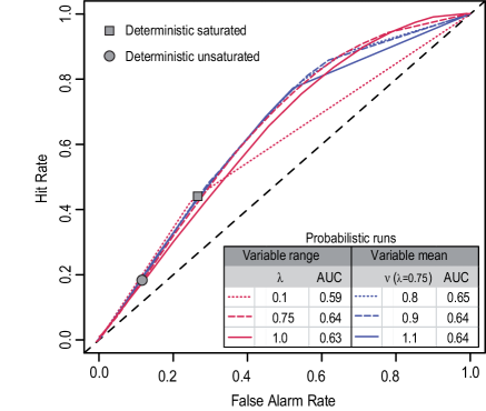
Abbildung 10: Frontignano study area. Maps of the factor of correct assignments and model error obtained within the probabilistic approach of TRIGRS-P, with the following values of range of variation of input parameters: (A) $\lambda=0.01$, $\nu=1.0$; (B) $\lambda=0.75$, $\nu=1.0$; (C) $\lambda=1.0$, $\nu=1.0$. (D) $\lambda=0.75$, $\nu=0.8$; (E) $\lambda=0.75$, $\nu=0.9$; (D) $\lambda=0.75$, $\nu=1.1$. TP, True Positive; TN, True Negative; FP, False Positive; FN False Negative. In all maps, black polygons show rainfall-induced landslides in the study area.

Abbildung 11: Frontignano study area; ROC plots corresponding to the runs with fixed input parameters (Figure 8b, c) and with the probabilistic approach with random input parameters (Figures 9 and 10).

including the True Positive Rate (sensitivity, or hit rate) ${\text{TPR}}={\text{TP}}/({\text{TP}}+{\text{FN}})$, the True Negative Rate (specificity) ${\text{TNR}}={\text{TN}}/({\text{FP}}+{\text{TN}})$, the False Positive Rate ($1$ – specificity, or false alarm rate) ${\text{FPR}}={\text{FP}}/({\text{FP}}+{\text{TN}})$, the Accuracy ${\text{ACC}}=({\text{TP}}+{\text{TN}})/({\text{TP}}+{\text{FN}}+{\text{FP}}+{\text{TN}})$, and the Precision ${\text{PPV}}={\text{TP}}/({\text{TP}}+{\text{FP}})$ (Fawcett, 2006; Baum et al., 2010).

2.1.2 Predictions with the probabilistic approach

Based on the comparison of the results discussed in the previous section, for the probabilistic modeling we used only the unsaturated soil conditions, and we exploited the same geomorphological information (i.e., the same DEM) and the same rainfall forcing input (i.e., $4.5\,\unit{mm\,h^{-1}}$ of rain for a 28-h period) used for the previous runs. For the mechanical and hydrological properties of the geological materials ($\phi$, $c$, ${\gamma}_{\mathrm{s}}$, $K_{\mathrm{s}}$, $D_{0}$, ${\theta}_{\mathrm{r}}$, ${\theta}_{\mathrm{s}}$) we considered the values listed in Table 1, used in the previous paragraph as fixed inputs of the model, as mean values of uniformly distributed variables ${\mathcal{U}}(y_{a},y_{b})$,

Tabelle 3: Estimators of model performance of the results obtained with the TRIGRS-P code in the Mukilteo study area. In this case we change the ranges of variation of the model parameters $\lambda$, with fixed mean values of the model parameters $\nu=1.0$. TPR, True Positive Rate; FPR, False Positive Rate; ACC, Accuracy; PPV, Precision; AUC, Area Under the ROC curve.

$\lambda$	TPR	FPR	ACC	PPV	AUC
$0.01$	$0.41$	$0.11$	$0.84$	$0.29$	$0.65$
$0.10$	$0.41$	$0.11$	$0.84$	$0.29$	$0.70$
$0.50$	$0.40$	$0.12$	$0.83$	$0.28$	$0.73$
$0.75$	$0.34$	$0.11$	$0.83$	$0.26$	$0.71$
$1.00$	$0.09$	$0.04$	$0.87$	$0.22$	$0.67$

where $y_{a}$ and $y_{b}$ are the lower and upper limits of the uniform distribution determining the range of variation of each parameter. In our simulations, the range of variation of the individual parameters has been chosen as a fraction of the mean value of each variable. A range of variation $\lambda=0.01$, 0.10 and 1.00 correspond to a variation of $1\,\unit{\%}$, $10\,\unit{\%}$ and $100\,\unit{\%}$ around the mean value of the variable, respectively. Note that the case with $\lambda=0.01$ allows the various input parameters to vary in a very limited range, and it can be seen as a test of our code: the original TRIGRS results with fixed input parameters should be obtained.

We performed two sets of runs. In the first set, the mean values of the mechanical and hydrological parameters (Table 1) were kept constant, and the range of variation of the individual parameters was modulated using $\lambda=0.01$, 0.1, 0.5, 1.0. In the second set, a fixed range of variation for the individual parameters was selected, $\lambda=1.0$, and the mean value of the parameters was modified (shifted) by $\nu=0.2$, $0.4,\dots,1.0$, 2.0. Note that when $\nu=1.0$, no shift of the mean value is performed. In each test, the same range of variation $\lambda$ and the same shift of the mean value $\nu$ were applied to all the parameters. The simplification was adopted to reduce the time required to perform multiple runs. The results are shown in Figure 4: (i) for the first set of runs, i.e. for fixed mean values of the model parameters and changing ranges of variation of the individual parameters, $\lambda=0.01$ (Figure 4a), $\lambda=0.5$ (Figure 4b), and $\lambda=1.0$ (Figure 4c), and (ii) for the second set of runs, i.e. for a fixed range of variation $\lambda=1.0$, and shifting the mean value of the model parameters by $\nu=0.8$ (Figure 4d), $\nu=0.9$ (Figure 4e), and $\nu=1.1$ (Figure 4e). For the second set of runs, results obtained for $\nu<0.8$ and for $\nu>1.1$ are not shown in Figure 4. For $\nu<0.8$ the number of unconditionally unstable cells was unrealistically large, and for $\nu>1.1$ the model performance decreased rapidly (see next paragraph). We used 16 runs for each set, resulting in 16 different maps of the factor of safety, which were used to evaluate the performance of the probabilistic approach. The results are shown in Figure 5.For the same runs of Figure 4, the maps show the geographical distribution of the correct assignments (TP, TN), the model errors (FP, FN), and the corresponding four-fold plots. Tables 3 and 4 list metrics that quantify

Tabelle 4: As in Table 3, but with fixed ranges of variation of and with varying the mean values the model parameters, for the Mukilteo area.

$\nu$	TPR	FPR	ACC	PPV	AUC
$0.8$	$0.77$	$0.46$	$0.56$	$0.16$	$0.73$
$0.9$	$0.57$	$0.23$	$0.75$	$0.22$	$0.73$
$1.0$	$0.40$	$0.12$	$0.83$	$0.27$	$0.73$
$1.1$	$0.23$	$0.06$	$0.87$	$0.31$	$0.72$

Abbildung 12: Maps showing the minimum (left column), maximum (centre column), and standard deviation (right column), of the factor of safety $F_{\mathrm{S}}$ for the set of 16 simulation runs using the TRIGRS-P code. Maps are shown for the Mukilteo (upper row) and the Frontignano (lower row) study areas.

the performance of the probabilistic approach.

2.1.3 Analysis and discussion

Inspection of the results of the deterministic (Figure 3) and the probabilistic (Figures 4 and 5) models, and of their forecasting skills (Figure 6, Tables 2–4), allows for general considerations. Figure 6 shows a Receiver Operating Characteristics (ROC) plot (Fawcett, 2006), defined by the false alarm rate FPR and the hit rate TPR, plotted on the x- and y-axes, respectively. In the ROC space, a point located in the upper left corner represents a perfect prediction (${\text{TPR}}=1$ and ${\text{FPR}}=0$), and points along the diagonal line for which ${\text{TPR}}={\text{FPR}}$ represent random predictions. An acceptable prediction requires ${\text{TPR}}/{\text{FPR}}>1$ (Fawcett, 2006). In Figure 6, two separate points show the predictive performance of the two runs with deterministic inputs, for saturated (Figure 3b) and for unsaturated (Figure 3c) conditions each of them producing a single pair FPR-TPR and a unique geographical distribution of the factor of safety $F_{\mathrm{S}}$. Analysis of Figures 3 and 6, and of Table 2 indicates that the model prepared considering the soil unsaturated conditions (Figure 3c) performed better than the model prepared considering saturated conditions (Figure 3b). The larger value of the TPR$/$FPR ratio is a measure of the better predicting performance of the unsaturated model (${\text{TPR}}/{\text{FPR}}=3.46$, Figure 6), compared to the saturated model (${\text{TPR}}/{\text{FPR}}=1.87$, Figure 3), despite a lower TPR value (${\text{TPR}}=0.42$ vs. ${\text{TPR}}=0.71$, Table 2). This is in agreement with previous work of Godt et al. (2008) and Baum et al. (2010).

Within the two deterministic models, the one using the unsaturated soil conditions (Figure 3c, f) performed better than the model that used the saturated soil conditions (Figure 3b, e). The saturated model predicted a significantly larger fraction of the study area as unstable, mainly where terrain gradient exceeded $15{\degree}$. This resulted in a considerably larger number of true positives (TP, 7.1 % vs. 4.1 %), but also a significantly larger number of false positives (FP, 33.8 % vs. 10.4 %) and a correspondingly significantly lower number of true negatives (TN, 56.1 % vs. 79.5 %). In other words, the saturated deterministic model (Figure 3b) was more pessimistic than the unsaturated deterministic model (Figure 3c). This is well represented in Figure 6, where a reduction of the false positive rate from 0.38 to 0.12 results in a reduction of the hit rate from 0.71 to 0.41 (Table 2). The subsequent runs with probabilistic input were obtained assuming unsaturated soil water conditions. The results of the unsaturated probabilistic models (Figure 4) were similar to the results of the corresponding unsaturated deterministic model (Figure 3c). This is a significant result, confirming that treating the uncertainty associated with the model parameters with a probabilistic approach has not significantly changed the model results, which have remained consistent. Availability of multiple model outputs for each run allowed preparing ROC curves to measure quantitatively the predictive performance of the probabilistic models (Fawcett, 2006). Since multiple values of $F_{\mathrm{S}}$ are available for each pixel in the modeling domain, we can calculate the frequency of stability condition of each pixel. We attribute to this frequency the meaning of a probability and compare it with a given threshold. Modulation of the classification threshold allows us to obtain different FPR and TPR values, which can be used to construct a ROC curve (Fawcett, 2006). In Figure 6 two sets of ROC curves are shown using different colors. The red curves show the performances of the first set of runs, for $\lambda=0.01$, $\lambda=0.5$, and $\lambda=1.0$, with $\nu=1.0$, and the blue curves show the performances of the second set of runs, for $\nu=0.8$, $\nu=0.9$, and $\nu=1.1$, with $\lambda=0.5$. To construct the ROC curves, several probability thresholds were used, from $0.1$ to $0.9$ by $0.1$ steps. The area under the ROC curve AUC is taken as a quantitative measure of the performance of the classification. If ${\text{AUC}}=0.5$, a classification is poor and indistinguishable from a random classification, whereas a perfect classification has ${\text{AUC}}=1$ (Fawcett, 2006; Rossi et al., 2010).

Inspection of Figures 5 and 6, and of Table 3, suggests that an increase in the range of variation of the model parameters (from $\lambda=0.01$ to $\lambda=1.0$), corresponding to a significantly larger degree of uncertainty in the parameters, resulted in similar individual performance indices, but significantly larger values of the area under the ROC curve, AUC. In our experiment, the increase in the range of variation changed the performance index from ${\text{AUC}}=0.65$ (for $\lambda=0.01$) to ${\text{AUC}}=0.73$ (for $\lambda=0.5$), with an increase of performance of 16 %. A further increase of the range of variation to $\lambda=1.0$, a possibly unrealistic range of variation for some of the modeling parameters, has resulted in a value of ${\text{AUC}}=0.67$, decreasing the model performance. Modulation of the mean value of the parameters, using $\nu=0.8$, $\nu=0.9$, and $\nu=1.1$, resulted in better results (larger AUC values) for $\lambda=0.5$ than for $\lambda=0.01$. Moreover, the TPR, FPR, PPV and ACC metrics did not change significantly when the range of variation $\lambda$ of the model parameters were modified, and remained similar to the values obtained with the deterministic models, for $\lambda\leq 0.5$. We conclude that, in the Mukilteo study area, these metrics are not sensitive to introduction of the probabilistic determination of the model parameters. Second, the AUC showed a positive correlation with the range of variation in the model parameters.

In the probabilistic runs, a positive correlation was observed between the range of variation $\lambda$ and the fraction of unconditionally unstable cells i.e., the grid cells that have $F_{\mathrm{S}}<1$ even in dry conditions when no rainfall is increasing pore pressure and slope instability. For the first set of runs, the fraction of unconditionally unstable cells was $0\,\unit{\%}$ for $\lambda=0.01$, $0.3\,\unit{\%}$ for $\lambda=0.5$, and $0.7\,\unit{\%}$ for $\lambda=1.0$. Moreover, a negative correlation was observed between $\nu$, the width of shift in the mean value of the modeling parameters, and the fraction of unconditionally unstable cells. For the second set of runs, the fraction of unconditionally unstable cells was less than $5.0\,\unit{\%}$ for $\nu\geq 0.8$, and was $0\,\unit{\%}$ for $\nu>1.0$, independent of the range of variation of the parameters.

2.2 Frontignano study area

The Frontignano area is located in central Umbria, Italy, about $25\,\unit{km}$ south of Perugia, in the Collazzone area (Figure 7). In this area, landslides are caused primarily by rainfall and rapid snowmelt (Cardinali et al., 2000; Guzzetti et al., 2006a, b; Fiorucci et al., 2011). Multiple deep-seated and shallow slides were identified in the area through the visual interpretation of multiple sets of aerial photographs and very-high resolution satellite images, and field surveys.

The shallow failures are typically less than three meters thick, and involve the soil and the colluvium mantling the slopes. Soils range in thickness from a few decimetres to more than one meter; they have a fine to medium texture, and exhibit a xeric moisture regime, typical of the Mediterranean climate. In central Umbria, precipitation is most abundant in October and November, with a mean annual rainfall in the period 1921–2001 exceeding 850 mm. In the study area, terrain is hilly, and the lithology and the attitude of bedding planes control the morphology of the slopes. Gravel, sand, clay, travertine, layered sandstone and marl, and thinly layered limestone, crop out in the area (Cardinali et al., 2000; Guzzetti et al., 2006a, b).

2.2.1 Predictions with the deterministic approach

For modeling purposes, the topography of the Frontignano study area was described by a $5\,\unit{m}\times 5\,\unit{m}$ DEM obtained interpolating $5$-m contour lines shown on $1:10\,000$ scale topographic base maps (Guzzetti et al., 2006a, b). Slope in the area ranges from $0{\degree}$ to $62{\degree}$, with an average value of $10{\degree}$ and a standard deviation of $5.6{\degree}$ (Figure 8d). The mechanical and hydrological properties of the five soil types cropping out in the area (Figure 8a) were determined through laboratory tests and searching the literature (see, e.g. Shafiee, 2008; Feda, 1995; Lade, 2010, and references therein) on the geotechnical properties ($\phi$, $c$, ${\gamma}_{\mathrm{s}}$, $K_{\mathrm{s}}$, $D_{0}$, ${\theta}_{\mathrm{r}}$, ${\theta}_{\mathrm{s}}$) of the same or similar sediments in Umbria, Italy (listed in Table 5). As for the Mukilteo area, the depth to the hypothetical sliding plane $d_{\text{fp}}$ was assumed to coincide with the soil depth, which was estimated using the model proposed by DeRose (1996). To calibrate the soil depth model, we exploited field observations indicating that the depth of the shallow landslides in the study area is $d_{\text{fp}}<3$ m, and that shallow landslides are most abundant where terrain gradient is in the range $7{\degree}\leq\delta\leq 20{\degree}$. Initial depth to the water table was set to a fraction of the depth to the failure plane, ${d_{\mathrm{w}}=0.85d}_{\text{fp}}$. Since the depth of the water table is an important initial condition for the model, we decided to use a long rainfall period, starting from an almost dry initial condition and reaching a realistic depth of the water table during the storm. We further decided not to set the water table to the maximum soil depth to consider the fact that the simulation is intended to be representative of typical winter conditions, when landslides occur in both study areas, and when the soil always contains some amount of water. We tested different rainfall histories, and adopted a forcing rainfall that produced shallow landslides in the area in the periods January–May 2004, October–December 2004, and October–December 2005 (Guzzetti et al., 2009; Fiorucci et al., 2011). Specifically, we used a rainfall history composed of a $4$-week initial rainfall period characterized by a constant mean rainfall intensity $I=0.36\,\unit{mm\,h^{-1}}$, for a cumulative rainfall $E=242\,\unit{mm}$, followed by a $60$-min rainfall period characterized by a high rainfall intensity $I=90\,\unit{mm\,h^{-1}}$, for a cumulative rainfall $E=90\,\unit{mm}$. Results for the saturated (Equation 4) and the unsaturated (Equation 5) modeling conditions are shown in Figures 8b, c, respectively.

To test the model performance, the geographical distribution of the factor of safety $F_{\mathrm{S}}$ predicted by TRIGRS were compared to the known distribution of rainfall-induced landslides mapped in the same area in the periods January to May 2004, October to December 2004, and October to December 2005. The landslides were mapped through reconnaissance fieldwork and the visual interpretation of high-resolution satellite images (Guzzetti et al., 2009; Fiorucci et al., 2011), and are shown with black lines in Figure 8. For the comparison, all grid cells with $F_{\mathrm{S}}<1$ were considered unstable (i.e., landslide) cells. As for the Mukilteo test case, four-fold plots (Figure 8e, f) and derived metrics (Table 6), ROC plots (Figure 11), and maps showing the geographical distribution of the correct assignments and the model errors (Figure 8e, f) were used to summarize and measure the comparison.

Inspection of Figures 8 and 11, and analysis of Table 6, suggests that the saturated and the unsaturated models produce very similar results. This is different from the result obtained in the Mukilteo area, where the unsaturated model performed better than the saturated model. In the Frontignano area, the unsaturated model (Figure 8c) resulted in a better forecasting accuracy (ACC, 0.86 vs. 0.75), but in a reduced TPR to FPR ratio ($1.4$ vs. $1.7$). We maintain that the model prepared considering the saturated conditions (Figure 8b) performed slightly better than the model obtained considering the unsaturated conditions (Figure 8c).

2.2.2 Predictions with the probabilistic approach

The mechanical and hydrological properties of the geological materials ($\phi$, $c$, ${\gamma}_{\mathrm{s}}$, $K_{\mathrm{s}}$, $D_{0}$, ${\theta}_{\mathrm{r}}$, ${\theta}_{\mathrm{s}}$) in the Frontignano study area were chosen as listed in Table 5 (also used as input of the original TRIGRS model, in the previous paragraph) as mean values of uniformly distributed variables ${\mathcal{U}}(y_{a},y_{b})$. To be consistent with the approach adopted in Mukilteo, we performed two sets of parametric analyses, varying the range ($\lambda$) and the mean value ($\nu$) of the model parameters. The maps in Figure 9 show the factor of safety $F_{\text{S}}$ calculated

Abbildung 13: Histograms showing the distribution of the values of the $F_{\mathrm{S}}$ for the Mukilteo (left, A, B, C) and the Frontignano (right, D, E, F) study areas. (A) and (D) for subsets of $1000$ grid cells with $0<\overline{F}_{\mathrm{S}}\leq 1.5$. (B) and (E) for subsets of $1000$ grid cells with $1.5<\overline{F}_{\mathrm{S}}\leq 3$. (C) and (F) for subsets of 1000 grid cells with such that $\overline{F}_{\mathrm{S}}>3$.

for: (i) fixed mean values of the model parameters $\nu=1.0$, and changing ranges of variation of the individual parameters, $\lambda=0.01$ (Figure 9a), $\lambda=0.75$ (Figure 9b), and $\lambda=1.0$ (Figure 9c), and (ii) a fixed range of variation $\lambda=0.75$, and shifting the mean value of the model parameters by $\nu=0.8$ (Figure 9d), $\nu=0.9$ (Figure 9e), and $\nu=1.1$ (Figure 9f). As in the previous case, $\lambda=0.01$ corresponds to a very small range of variability of the parameters, and provides the same results. For $\nu=1.0$, no shift in the mean values of the model parameters is performed. The degree of accuracy of the two sets of runs for the Frontignano area is shown in Figure 10, for the same models shown in Figure 9. The maps show the geographical distribution of the correct assignments (TP, TN), the model errors (FP, FN), and the corresponding four-fold plots. Tables 7 and 8 list metrics that quantify the performance of the runs. The performance of the probabilistic models is further analysed in Figure 11 by two sets of ROC curves, shown using different colours; red curves for the case of variable range $\lambda$, and blue curves for the case of a variable mean $\nu$. In the same plot, the grey circle shows the predicting performance of the saturated model (Figure 8b), and the grey square the performance of the unsaturated model (Figure 8c) both run with fixed input parameters.

2.2.3 Analysis and discussion

Inspection of the results of the fixed input runs (Figure 8), the runs with input parameter sampled from a suitable probability distribution, (Figures 9 and 10), and of their ability to forecast the spatial distribution of known landslides (Figure 11, Tables 6–8), allows for considerations that are similar to those discussed for the Mukilteo study area (see Sect. 3.1.3), with a few differences. In the Frontignano area, the saturated and the unsaturated models provided nearly equivalent results, with the saturated model considered marginally superior primarily because of the reduced value of the TPR to FPR ratio. From a statistical point of view, given the reduced fraction of landslide area in Frontignano ($1.5\,\unit{\%}$) compared to Mukilteo ($4.2\,\unit{\%}$), the spatial prediction of landslides in Frontignano was more difficult than in Mukilteo. From a physical point of view, modeling the stability conditions in low gradient terrain is very sensitive to the initial conditions, which are uncertain and difficult to determine spatially. The runs with variable input parameters confirm the slightly poorer geographical predictive performance of the adopted physical framework in Frontignano, compared to Mukilteo (Tables 3 and 4 vs. Tables 7 and 8). Taking the area under the ROC curve (AUC) as the metric to compare the models, one can readily see that runs for the Mukilteo area resulted in $0.65\leq{\text{AUC}}\leq 0.73$, and for the Frontignano area exhibited $0.59\leq{\text{AUC}}\leq 0.65$. In other words, the “worst” result for Mukilteo (${\text{AUC}}=0.65$, for $\nu=1.0$ and $\lambda=0.01$) has the same overall spatial predictive performance of the “best” result for Frontignano (${\text{AUC}}=0.65$, for $\nu=0.8\ or\ 0.9$ and $\lambda=0.75$). In the Frontignano area, despite a lower “absolute” performance (i.e., when compared to Mukilteo), adoption of a probabilistic approach improved the spatial forecasting skills. Again, taking AUC as a metric to compare the models, values of this metric increased from ${\text{AUC}}=0.59$ (for $\nu=1.0$ and $\lambda=0.01$), to ${\text{AUC}}=0.65$ (for $\nu=0.8$ or 0.9 and $\lambda=0.75$). This is a non-negligible improvement of about $10\,\unit{\%}$. The result confirms that adoption of a probabilistic framework to the distributed modeling of shallow landslides results in improved spatial forecasts.

The result further corroborates the finding that modeling the natural uncertainty (and poor understanding) of the mechanical and hydrological variables results in better spatial landslide predictions of the locations of rainfall-induced landslides (see insets in Figure 4). First, the TPR, FPR, PPV, and AUC metrics did not change significantly when the range of variation $\lambda$ of the model parameters was changed. These metrics remained similar to the values obtained with the fixed input model, confirming

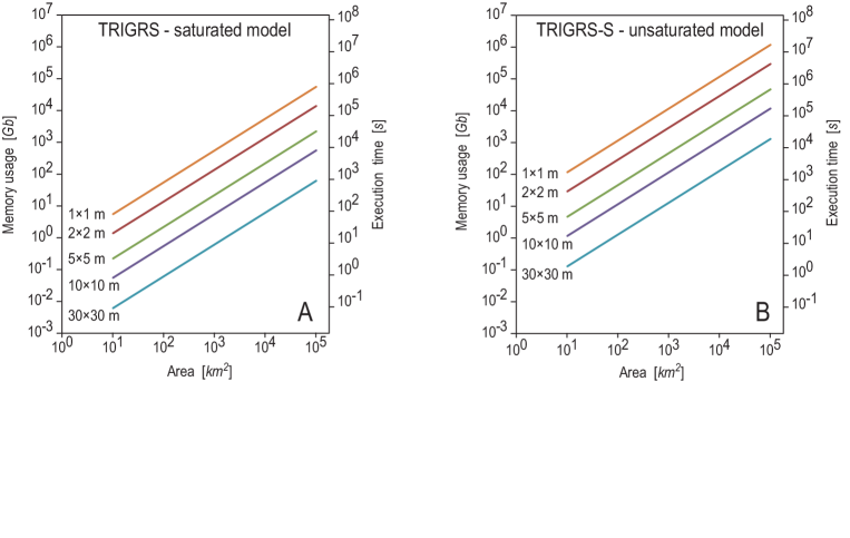
Abbildung 14: Estimated memory usage (left y-axis) and execution times (right y-axis) for (A) the TRIGRS code (saturated model), and (B) a set of 16 runs of the TRIGRS-P code, for areas of different extent, and for grid cells of different spaptial resolutions.

that they are not sensitive to differences between probabilistic framework runs with random variations of parameters and runs with fixed parameters. Second, the area under the ROC curve AUC confirmed its positive correlation with the range of variation in the model parameters $\lambda$, in support of the probabilistic approach. Third, the positive correlation between the range of variation $\lambda$ and the fraction of unconditionally unstable cells, and the negative correlation between the shift in the mean value of the modeling parameters $\nu$ and the fraction of unconditionally unstable cells, were both confirmed.

3 Discussion

Our probabilistic approach to the distributed modeling of shallow landslides proved effective in the two study areas where it was tested (Figures 2 and 7). In both areas, the maps showing the geographical distribution of the factor of safety $F_{\mathrm{S}}$ obtained using TRIGRS-P were better predictors of the distributions of known rainfall-induced landslides than the corresponding maps obtained adopting the original TRIGRS approach. This conclusion is supported by the indices used to measure the forecasting skills of the different models, and particularly the area under the ROC, AUC (Tables 2–4 for Mukilteo, and Table 6, 7, 8 for Frontignano). The runs in which we allowed a large variability of the input parameters (e.g. $\lambda=0.50$ or $\lambda=0.75$) were better predictors of the geographical distribution of known landslides than the models prepared using a reduced variability in the model parameters (e.g. $\lambda=0.1$) (Guzzetti et al., 2006a; Rossi et al., 2010). This is shown in the insets in Figure 4, where a portion of the results for the Mukilteo study area is shown at a larger scale. The variability of the geographical distribution of the $F_{\mathrm{S}}$ is also shown in Figure 12 where we have plotted the minimum, the maximum, and the standard deviation of the computed $F_{\mathrm{S}}$ values. In particular, the map of the standard deviation provides quantitative and spatially distributed evidence of the uncertainty associated with the distributed modeling of landslide instability.

We studied the variation of the computed factor of safety. Figure 13 shows histograms for the distribution of the values of the factor of safety $F_{\mathrm{S}}$ in selected grid cells in the Mukilteo (Figure 13a–c) and the Frontignano (Figure 13d–f) study areas. For simplicity, in the Figure we show the results obtained for a single lithological type i.e., the transition sediments (Qtb, indicated as unit $1$ in Table 1) in the Mukilteo area (Figure 3a), and the sand-silt-clay (unit 5 in Table 5) in the Frontignano area (Figure 8a). Results for other lithological types in the two study areas are similar. We adopted the following procedure to obtain the histograms. First, we performed $100$ probabilistic simulations to obtain a large set of values of the factor of safety $F_{\mathrm{S}}$, and we computed the average value of the factor of safety, $\overline{F_{\mathrm{S}}}$ for each grid cell in the two modeling domains. For both study areas, a value of $\lambda=0.50$ (and $\nu=1.0$) was used for the variability of the geotechnical and hydrological parameters. Next, we selected three subsets of 1000 grid cells, with $0<\overline{F}_{\mathrm{S}}\leq 1.5$, $1.5<\overline{F}_{\mathrm{S}}\leq 3.0$, and $\overline{F}_{\mathrm{S}}>3$, respectively. Finally, we used all the computed values of the $F_{\mathrm{S}}$ in each subset to construct the histograms. Inspection of the histograms reveals that for $\overline{F}_{\mathrm{S}}>3$ (Figure 13c, f) the distribution of the predicted factor of safety is almost uniform and does not show a predominant value. Instead, for $\overline{F}_{\mathrm{S}}<1.5$ the distribution of the predicted factors of safety peaks at $F_{\mathrm{S}}\approx 1.0$ (Figure 13a, d). For $1.5<\overline{F}_{\mathrm{S}}\leq 3.0$, results are intermediate (Figure 13b, e).

In conclusion, the probabilistic approach results in a number of model outputs, each representing the geographical distribution of the $F_{\mathrm{S}}$ values. In this work, 16 runs were performed. Availability of multiple results allows for the analysis of the sensitivity of the

Tabelle 5: Geotechnical parameters for the geological units cropping out in the Frontignano study area (Figure 8a). $c$, cohesion; $\phi$, friction angle; $D_{0}$, hydraulic diffusivity; $K_{\text{S}}$, saturated hydraulic conductivity; $\theta_{\mathrm{s}}$, saturated water content; $\theta_{\text{r}}$, residual water content; $\alpha$, inverse of capillary fringe. Geological units: $1$, sand; $2$, clay; $3$, flysch deposits; $4$, gravel, sand, silt, and clay; $5$, sand, silt, and clay.

Unit	$c$	$\phi$	$D_{0}$	$K_{\mathrm{s}}$	$\theta_{\mathrm{s}}$	$\theta_{\mathrm{r}}$	$\alpha$
	[kPa]	[deg]	[m2 s-1]	[m s-1]	–	–	[m-1]
$1$	$3.0$	$31$	$3.8\cdot 10^{-4}$	$1.0\cdot 10^{-4}$	$0.20$	$0.05$	$2$
$2$	$4.0$	$18$	$5.0\cdot 10^{-6}$	$1.0\cdot 10^{-7}$	$0.80$	$0.07$	$5$
$3$	$50.0$	$25$	$8.3\cdot 10^{-6}$	$1.0\cdot 10^{-6}$	$0.45$	$0.1$	$5$
$4$	$15.0$	$30$	$4.0\cdot 10^{-4}$	$1.0\cdot 10^{-4}$	$0.45$	$0.1$	$5$
$5$	$3.0$	$15$	$4.7\cdot 10^{-3}$	$1.0\cdot 10^{-4}$	$0.50$	$0.1$	$1$

model to variations in the input parameters controlling the stability conditions. Variability depends on multiple causes (Uchida et al., 2011), including: (i) the natural variability in the geotechnical and hydrological properties of the soils; (ii) the inability of determining accurate values for the geotechnical and hydrological parameters, and (iii) the fact that the models are simplified and do not represent the natural (physical) conditions in the study area.

The probabilistic approach allowed the investigation of the combined effects of the natural variability inherent in the model parameters, and of the uncertainty associated with their definition over large areas. However, the approach cannot separate the two causes for the variability. Also, the probabilistic approach cannot validate the physics in the model better than the deterministic approach. It should be noted that in our runs with probabilistic input parameters, the geotechnical and hydrological properties were treated explicitly as independent (uncorrelated) variables. This was a simplification. In reality, some dependence (correlation) exists between the different geo-hydrological properties. As an example, the saturated water content ${\theta}_{\mathrm{s}}$ affects the saturated hydraulic conductivity $K_{\mathrm{s}}$ and the hydraulic diffusivity $D_{0}$. However, selection of values for the different properties based on field tests, laboratory experiments, or through a literature search resulted in values for the considered properties that were implicitly dependent. This is because e.g., cohesion, angle of internal friction, soil unit weight, and hydraulic conductivity depend one upon the other. Furthermore, no spatial correlation of the individual variables was considered in the modeling. This was also a simplification, because spatial correlation exists between the geo-hydrological properties (e.g., Rodriguez-Iturbe et al., 1999; Western et al., 2004). Adoption of the uniform distribution to determine the possible range of

Tabelle 6: As in Table 2, but for the Frontignano area.

Model type	TPR	FPR	ACC	PPV
Saturated	$0.42$	$0.25$	$0.75$	$0.02$
Unsaturated	$0.18$	$0.13$	$0.86$	$0.02$

variation of the individual parameters, combined with the accepted modeling simplifications, has resulted in more “extreme” results, but not in unrealistic results.

Results of our approach were obtained adopting the uniform distribution to describe the uncertainty associated with the geo-hydrological parameters. TRIGRS-P allows for the use of the Gaussian and the uniform distributions. In the runs presented in this work, we explored only part of the variability associated with the physical model describing slope instability forced by rainfall infiltration (Figure 1b), and specifically the variability associated with the mechanical and hydrological parameters of the materials involved in the hypothetical landslides. We did not consider the local morphological variability, e.g. the uncertainty in the description of the terrain given by the DEMs. Terrain gradient is an important parameter for the computation of the factor of safety $F_{\mathrm{S}}$. Inspection of Equation (1) shows that variability in the terrain gradient $\delta$ results in variability in the local stability conditions, measured by $F_{\mathrm{S}}$. Furthermore, in our runs soil depth was a (non-linear) function of the local slope (DeRose, 1996; Salciarini et al., 2006). Variations in the slope will result in variations in soil thickness, and in the local stability conditions. Preliminary results obtained adding a uniform random perturbation to the DEM for the Frontignano area confirmed the (large) sensitivity of the physically based models to the topographic information (Montgomery and Dietrich, 1994; van Westen et al., 2008; Tarolli et al., 2012).

Rainfall history and geographical pattern also control the local stability/instability conditions, and their temporal and spatial variations. For Mukilteo, we used the measured rainfall history that triggered shallow

Tabelle 7: As in Table 3, but for the Frontignano area.

$\lambda$	TPR	FPR	ACC	PPV	AUC
$0.01$	$0.42$	$0.25$	$0.75$	$0.03$	$0.59$
$0.10$	$0.41$	$0.25$	$0.75$	$0.03$	$0.60$
$0.50$	$0.37$	$0.22$	$0.77$	$0.03$	$0.64$
$0.75$	$0.27$	$0.17$	$0.83$	$0.03$	$0.64$
$1.00$	$0.05$	$0.04$	$0.95$	$0.02$	$0.63$

Tabelle 8: As in Table 4, but for the Frontignano area.

$\nu$	TPR	FPR	ACC	PPV	AUC
$0.8$	$0.57$	$0.37$	$0.63$	$0.02$	$0.65$
$0.9$	$0.44$	$0.27$	$0.72$	$0.02$	$0.64$
$1.0$	$0.27$	$0.17$	$0.83$	$0.03$	$0.64$
$1.1$	$0.10$	$0.06$	$0.92$	$0.02$	$0.64$

landslides in the winter 1996–1997. For Frontignano, we used the rainfall history that has resulted in shallow landslides in the winter 2004–2005. However, sensitivity of the models to the temporal and spatial variation of rainfall was not investigated, as this was not within the scope of the work. The effects of changing rainfall histories was investigated by Alvioli et al. (2014), who examined storms of different durations and average intensities. The rainfall data used in the two runs were obtained from rain gauges located in the vicinity of the study areas. The rainfall measurements may not represent the exact amount of rainfall at each grid cell in the modeling domain. We further assumed a uniformly distributed rainfall in the geographical modeling domains. Runs performed in the Frontignano area adopting different rainfall histories (e.g., (i) a uniform rainfall rate of $0.36\,\unit{mm\,h^{-1}}$ for a $4$-week period, for a cumulated rainfall $E=242\,\unit{mm}$, (ii) a single rainfall event with $5\,\unit{mm\,h^{-1}}$ for 24 h, $E=121\,\unit{mm}$, and (iii) intermittent $3$-day rainfall periods with $I=1.0\,\unit{mm\,h^{-1}}$ separated by $4$-day dry periods, for a $4$-week period, $E=288\,\unit{mm}$) revealed that the geographical distributions of the $F_{\mathrm{S}}$ obtained with the different rainfall histories were similar. However, the local instability conditions ($F_{\mathrm{S}}\leq 1$) were reached at different times. The difference may be significant if the model results are used in a landslide early warning system (Aleotti, 2004; Godt et al., 2006). We did not evaluate the sensitivity of the model parameters to the different rainfall histories.

It should be noted that the probabilistic approach of TRIGRS-P could be used to infer reasonable values of the parameters describing terrain characteristics, where they are largely unknown, by exploring a large parameter space in a random way and comparing with known distributions of landslides.

Adoption of a probabilistic approach with multiple runs using randomly generated different set of input parameters results in longer computer processing times. The time required for a single TRIGRS-P simulation is only slightly longer than the time needed for the corresponding TRIGRS simulation, since the random variables were computed before running the slope stability and infiltration model. The time for this initial step depends on the size (in grid cells) and complexity of the modeling domain. The processing time of the multiple runs required by the TRIGRS-P approach to have a statistical significance may be easily reduced by exploiting the multi-core architecture of modern CPUs, just running simultaneously multiple instances of the TRIGRS-P code initialised with different sets of parameters. Since our aim is to eventually use the TRIGRS as a region-wide and possibly nation-wide early warning system, we give an estimate of the computing resources required. Using the same spatial resolution, a larger area will require a larger processing time, with the time increasing linearly with the number of grid cells. The time required for a simulation depends also on rainfall history. A more complex history (i.e., a shorter step between two subsequent inputs of rainfall intensity) will result in a longer processing time, with time increasing with the square of the time steps. Finally, processing time depends on the type of hydrological model used, with the saturated model requiring roughly half the time of the unsaturated model.

When using the probabilistic approach, we adopted a strategy based on a convergence level, $\eta$. First, we computed two probabilistic sets with $n$ and $m>n$ simulations. Next, for the two independent sets and for each grid cell, we computed the mean of the factor of safety $\overline{F}_{\mathrm{S}}$. Then, we obtained the difference of the mean values of the factor of safety $\Delta\overline{F}_{\mathrm{S}}$ for each cell, and we identified the maximum value of $\max(\Delta\overline{F}_{\mathrm{S}})$ in the modeling domain. If $\max(\Delta\overline{F}_{\mathrm{S}})\leq\eta$, the convergence level was reached and no additional simulations were performed. Instead, if $\max(\Delta\overline{F}_{\mathrm{S}})>\eta$ convergence was not reached, a larger probabilistic set was prepared, and the test repeated. In our two study areas 16 simulations were sufficient to obtain a convergence level $\eta=0.05$. This level was considered adequate for the two study areas. This may not be the case in other areas, in significantly large areas, or in areas characterized by a larger physiographical variability. For simulations covering large areas, we hypothesized areas extending between $10^{1}$ and $10^{5}\,\unit{km^{2}}$ with grids of resolution from $1\,\unit{m}\times 1\,\unit{m}$ to $30\,\unit{m}\times 30\,\unit{m}$, and computed the memory usage and execution time for (i) a single deterministic simulation adopting a saturated soil model (Figure 14a), and (ii) a probabilistic set of 16 simulations using an unsaturated soil model (Figure 14b).

Since the TRIGRS (and TRIGRS-P) model uses a cell-by-cell description of the study area, and the equations describing the stability of each cell are independent from the neighbouring cells behavior, the code is most suited for a parallel implementation using MPI libraries. We performed preliminary simulations, showing that a significant speedup ($\simeq 1/N$, with N the number of processing elements used) can be obtained for the computing-intensive portions of the code. One problem associated with significantly large areas is the use of memory. In a truly parallel implementation of the code, each computing element or core should load into memory only the portion of data relevant to its task, which is currently not implemented.

We prepared a probabilistic version of the Transient Rainfall Infiltration and Grid-Based Regional Slope-Stability Analysis code, TRIGRS (Baum et al., 2002, 2008), and tested the new code TRIGRS-P in two study areas: Mukilteo, near Seattle, USA, and Frontignano, near Perugia, Italy. The tests suggest that the runs initialized with random values of the input parameters generated according to proper probability distribution functions, were better predictors of the spatial location of rainfall-induced shallow landslides than the corresponding original TRIGRS runs. This was measured by different metrics used to evaluate the comparison of the spatial forecasts of the instability conditions ($F_{\mathrm{S}}$ values) against maps showing recent rainfall-induced landslides, in the two study areas. Adoption of a probabilistic-initiated framework allowed the investigation of the sensitivity of the model used to determine the stability conditions to the geotechnical and hydrological properties of the terrains where landslides can develop. The observed sensitivity was attributed to the combined effect of the natural variability inherent to the geotechnical and hydrological properties of the slope materials, and to the fact that the numerical model is an approximate representation of the complex processes controlling rainfall-induced slope instability in an area. However, the probabilistic approach cannot separate the two causes of variability. Probabilistic modeling of rainfall-induced shallow landslides requires longer processing times, when compared to the corresponding deterministic modeling. A parametric study proved that the approach is computationally feasible even for very large areas ($10^{4}\,\unit{km^{2}}$, $10^{8}$ grid cells) if a computer grid is used, and a parallel computing strategy is adopted. We expect the probabilistic approach to improve the current capability to forecast the occurrence of rainfall-induced shallow landslides, and to facilitate the investigation of the variability of slope material properties over large areas.

Anhang A Formulation of the model

In this appendix we summarize the solutions of Equation (2) implemented in deterministic code TRIGRS (Baum et al., 2010). Approximations are given for: (i) unsaturated soil conditions (Srivastava and Yeh, 1991), (ii) saturated soil conditions (Iverson, 2000), and (iii) a two-layer soil model (Baum et al., 2010) represented schematically in Figure 1b.

A.1 Unsaturated soil

In their model for an unsaturated soil, Srivastava and Yeh (1991) use relation (Equation 2) to linearize Equation (2). The explicit solution for the hydraulic conductivity (Equation 7), subject to the initial and boundary conditions given by Equation (8), is the following:

$$K(Z,t)=\, I_{\text{Z}}-\left[I_{\text{Z}}-K_{\mathrm{s}}\right]e^{-\alpha_{1}(d_{\mathrm{w}}-Z)}-4\left(I_{\text{Z}}-I_{ZLT}\right)e^{\frac{\alpha_{1}Z}{2}\,-D_{\psi}\frac{t}{4}}\,\sum_{m=1}^{\infty}\frac{\sin[\Lambda_{m}\alpha_{1}(d_{\mathrm{w}}-Z)]\sin(\Lambda_{m}\alpha_{1}d_{\mathrm{w}})}{1+\frac{\alpha_{1}d_{\mathrm{w}}}{2}+2\Lambda_{m}^{2}\alpha_{1}d_{\mathrm{w}}}\,\,e^{-\Lambda_{m}^{2}D_{\psi}t}$$ (12)

where ${\alpha}_{1}=\alpha\,{\cos}^{2}\delta$, $I_{ZLT}$ is the initial surface flux (where the subscript LT indicates the long term infiltration rate), $I_{Z}$ is the surface flux of a given intensity for the considered time interval, $D_{\psi}={\alpha}_{{1}}K_{\mathrm{s}}/({\theta}_{\mathrm{s}}-{\theta}_{\mathrm{r}})$ and ${\Lambda}_{m}$ are the positive roots of the pseudoperiodic characteristic equation ${\text{tan}}\left(\Lambda{\alpha}_{{1}}d_{\mathrm{w}}\right)+2\Lambda=0$. The pressure head $\psi\left(Z,t\right)$ in the unsaturated zone is obtained by inversion of Gardner (1958) equation, Equation (7):

$$\psi\left(Z,t\right)=\frac{\cos\delta}{\alpha_{1}}\ln\left[\frac{K(Z,t)}{K_{\mathrm{s}}}\right]+\psi_{0}$$ (13)

A.2 Saturated soil

For wet initial conditions, Iverson (2000) gave an explicit solution of the linearized Richards equation, for long term and for short term behavior. The long term represents the steady component:

$$\psi(z)=(z-d_{\mathrm{w}})\left[\cos\delta-\frac{I_{ZLT}}{K_{\mathrm{s}}}\right]$$ (14)

where $z=Z{\text{cos}}\delta$ and $d_{\mathrm{w}}$ is the depth to the water table (see Figure 1b). The short term represents the transient component:

$$\psi(Z,t\leq T)=(Z-d_{\mathrm{w}})\beta++\frac{I_{Z}}{K_{\mathrm{s}}}\left[\left(\frac{\bar{D}t}{\pi}\right)^{\frac{1}{2}}e^{-\frac{Z^{2}}{\bar{D}t}}\right.\left.-Z\,{\text{erfc}}\,\left(\frac{Z^{2}}{\bar{D}t}\right)\right]$$ (15)

$$\psi(Z,t>T)=\psi(Z,t\leq T)-\frac{I_{Z}}{K_{\mathrm{s}}}\left[\left(\frac{\bar{D}(t-T)}{\pi}\right)^{\frac{1}{2}}e^{-\frac{Z^{2}}{\bar{D}(t-T)}}\right.\left.-Z\,\,{\text{erfc}}\,\,\left(\frac{Z^{2}}{\bar{D}(t-T)}\right)\right]$$ (16)

Tabelle 9: Notation.

Symbols	Description
$A$:	Upslope contributing area, $L^{2}$.
$c$:	Soil cohesion, $ML^{-1}T^{-2}$.
$C$:	Specific moisture capacity, $L^{-1}$.
$C_{0}$:	Moisture capacity at saturation, $L^{-1}$.
$d_{\mathrm{w}}$:	Depth to the water table, $L$.
$d_{\text{fp}}$:	Depth to the sliding plane, $L$.
$D_{0}$:	Saturated hydraulic diffusivity, $L^{2}T^{-1}$.
$E$:	Cumulated event rainfall, $L$.
$F_{\mathrm{S}}$:	Factor of safety [–].
$\overline{F}_{\mathrm{S}}$:	Average value of the factor of safety [–].
$I$:	Mean rainfall intensity, $LT^{-1}$.
$K_{x}$:	Hydraulic conductivity in $x$ direction, $LT^{-1}$.
$K_{y}$:	Hydraulic conductivity in $y$ direction, $LT^{-1}$.
$K_{z}$:	Hydraulic conductivity in $z$ direction, $LT^{-1}$.
$K_{\mathrm{s}}$:	Saturated hydraulic conductivity, $LT^{-1}$.
$K^{*}$:	Normalized hydraulic conductivity [–].
$n$:	Number of simulations in a probabilistic set.
$t$:	Time, $T$.
$t^{*}$:	Normalized time [–].
${\mathcal{N}}(0,1)$:	Standard normal distribution.
${\mathcal{U}}(0,1)$:	Standard uniform distribution.
${\mathcal{N}}(\overline{x},{\sigma}_{x})$:	Normal distribution.
${\mathcal{U}}(\overline{y},\lambda)$:	Uniform distribution.
$x$:	Slope parallel coordinate, $L$.
$\overline{x}$:	Mean value of the generic variable $x$.
$y$:	Slope parallel coordinate, orthogonal to $x$, $L$.
$\overline{y}$:	Mean value of the generic variable $y$, $L$.
$y_{a},y_{b}$:	Minimum and maximum values for the generic variable $y$, $L$.
$z$:	Slope normal coordinate, $L$.
$z^{*}$:	Normalized slope normal coordinate [–].
$Z$:	Vertical coordinate, $Z=z/\cos\delta$, $L$.
$\alpha$:	Parameter for fitting soil-water characteristic curve, $L^{-1}$.
${\gamma}_{\mathrm{w}}$:	Unit weight of water, $ML^{-2}T^{-2}$.
${\gamma}_{\mathrm{s}}$:	Unit weight of soil $ML^{-2}T^{-2}$.
$\delta$:	Slope angle, corresponds to gradient of the sliding plane [–].
$\varepsilon$:	Ratio of length scales for slope-normal and lateral infiltration.
$\theta$:	Volumetric water content [–].
${\theta}_{\mathrm{s}}$:	Saturated water content [–].
${\theta}_{\mathrm{r}}$:	Residual water content [–].
$\lambda$:	Range of the random variable $y$, $L$.
$\sigma$:	Standard deviation for a normally distributed variable, $L$.
${\sigma}_{x}$:	Standard deviation for the normally distributed variable $x$, $L$.
$\phi$:	Soil friction angle [–].
$\psi$:	Groundwater pressure head, $L$.
${\psi}^{*}$:	Normalized groundwater pressure head [–].
$\widetilde{\psi}$:	Pressure head in Gardner’s model, $L$.
$\xi$:	Generic random variable.

where $T$ is the rainfall duration, $\overline{D}=4D_{0}\cos^{2}\delta$ is an effective hydraulic diffusivity, and erfc is the complementary error function:

$${\text{erfc}}\,(x)=1-\,{\text{erf}}\,(x)=\frac{2}{\sqrt{\pi}}\int_{x}^{\infty}e^{-t^{2}}\;\mathrm{d}t$$ (17)

A.3 Two-layer soil model

The linearized Richards equation allows for the superposition of solutions. Baum et al. (2002) have extended the Iverson (2000) and the Srivastava and Yeh (1991) solutions to the case of a time-varying sequence of surface fluxes with variable intensity and duration. They also considered an unsaturated layer of depth $d$ and depth to the top of the capillary fringe $d_{u}$ (see Figure 1b). Solution of Equation (12) was generalized as follows:

$$K(Z,t) =\sum_{n=1}^{N}H(t-t_{n})\left\{I_{nZ}-\left[I_{nZ}-K_{\mathrm{s}}\right]e^{-\alpha_{1}(d-Z)}-4\left(I_{Z}-I_{ZLT}\right)e^{\frac{\alpha_{1}Z}{2}}e^{-D_{\psi}\frac{t-t_{n}}{4}}\,\cdot\right.$$

$$\cdot\left.\sum_{m=1}^{\infty}\frac{\sin\left[\Lambda_{m}\alpha_{1}(d-Z)\right]\sin\left(\Lambda_{m}\alpha_{1}d\right)}{1+\frac{\alpha_{1}d}{2}+2\Lambda_{m}^{2}\alpha_{1}d}e^{-\Lambda_{m}^{2}D_{\psi}(t-t_{n})}\right\}\,+$$

$$-\,\sum_{n=1}^{N}H(t-t_{n+1})\left\{I_{nZ}-\left[I_{nZ}-K_{\mathrm{s}}\right]e^{-\alpha_{1}(d-Z)}-4\left(I_{Z}-I_{ZLT}\right)\cdot\right.$$

$$\left.\cdot\,e^{\frac{\alpha_{1}Z}{2}}e^{-D_{\psi}\frac{t-t_{n+1}}{4}}\sum_{m=1}^{\infty}\frac{\sin\left[\Lambda_{m}\alpha_{1}(d-Z)\right]\sin\left(\Lambda_{m}\alpha_{1}d\right)}{1+\frac{\alpha_{1}d}{2}+2\Lambda_{m}^{2}\alpha_{1}d}\,e^{-\Lambda_{m}^{2}D_{\psi}(t-t_{n+1})}\right\}$$ (18)

where $I_{nZ}$ is the surface flux of a given intensity for the $n$-th time interval, and $H(t-t_{n})$ is the Heaviside step function. The Iverson (2000) solutions of Eqs. (15) and (16) are generalized as:

$$\psi(Z,t)=\, (Z-d)\beta+2\sum_{n=1}^{\text{N}}\frac{I_{nZ}}{K_{\mathrm{s}}}\left\{H(t-t_{n})\left[D_{1}(t-t_{n})^{\frac{1}{2}}\right]i\,{\text{erfc}}\,\,\left[\frac{Z}{2[D_{1}(t-t_{n})]^{\frac{1}{2}}}\right]\right\}\,+$$

$$-2\sum_{n=1}^{\text{N}}\frac{I_{nZ}}{K_{\mathrm{s}}}\left\{H(t-t_{n+1})\left[D_{1}(t-t_{n+1})^{\frac{1}{2}}\right]\,i\,{\text{erfc}}\,\,\left[\frac{Z}{2[D_{1}(t-t_{n+1})]^{\frac{1}{2}}}\right]\right\}$$ (19)

with ${\text{ierfc}}(\eta)=\frac{1}{\sqrt{\pi}}\exp(-{\eta}^{{2}})-\eta{\text{erfc}}(\eta)$.

zip