Space Decompositions and Solvers for Discontinuous Galerkin Methods

Abstract

We present a brief overview of the different domain and space decomposition techniques that enter in developing and analyzing solvers for discontinuous Galerkin methods. Emphasis is given to the novel and distinct features that arise when considering DG discretizations over conforming methods. Connections and differences with the conforming approaches are emphasized.

1 Introduction

The design and the analysis of efficient preconditioners for discontinuous Galerkin discretizations has been subject of intensive research in the last decade with efforts focused mainly on elliptic problems.

A standard point of view when studying most of the preconditioning and iterative solution strategies, in general, is associated with a particular space decomposition. From the classical theory of Lions ayusob_plenary_lions1 ; ayusob_plenary_toselli-widlund ; ayusob_plenary_XZ , we know that, the choice of the space decomposition plays significant role in the construction and also in the convergence properties of the resulting preconditioners. For nonconfoming methods, domain decomposition and multigrid preconditioners have been analyzed by establishing connections with their respective conforming sub-spaces ayusob_plenary_brennerNC ; ayusob_plenary_Oswald96 . In the case of DG methods, the discontinuous nature of the DG finite element spaces allows to introduce and study not only space splittings pertinent to the conforming methods but also consider new splittings which give rise to new techniques and ideas.

In most of the earlier works, relevant space splittings of the DG finite element space, were introduced via a domain decomposition. Overlapping additive Schwarz methods have been studied following the classical Schwarz theory for different DG schemes ayusob_plenary_kara0 ; ayusob_plenary_bren10 ; ayusob_plenary_wid0 . Contrary to the conforming case, additive (and multiplicative) Schwarz methods based on non-overlapping decomposition of the computational domain have been constructed and proven to be convergent for DG methods. For such type of preconditioners, novel features, which have no analog in the conforming case, arise. For both overlapping and non-overlapping Schwarz methods, the splittings are stable in the $L^{2}$-norm by construction and can be shown to be stable in the natural DG energy norm, with constants depending on the mesh sizes relative to the coarse and fine subspaces.

More sophisticated substructuring preconditioners have been studied recently for two dimensional elliptic Poisson problems. In ayusob_plenary_sarkis0 ; ayusob_plenary_sarkis1 ; ayusob_plenary_sarkis2 ; ayusob_plenary_noi non-overlapping BDDC, N-N, FETI-DP and BPS domain decomposition preconditioners are introduced and analyzed for a Nitsche-type approximation. BDDC preconditioners are studied in ayusob_plenary_luca ; ayusob_plenary_Joachim for IP-spectral and IP-hybridized methods. Also here, several different approaches have been considered and new theoretical tools have been introduced. And of course, the space splitting in which the preconditioner rely, comes always from domain decomposition. Starting directly with a splitting of the DG space, dictated by a hierarchy of meshes, multigrid methods have been proposed and analyzed in ayusob_plenary_GK ; ayusob_plenary_brennerMGIP . A different approach was taken in ayusob_plenary_dobrev and ayusob_plenary_dahmen1 ; ayusob_plenary_kolja1 , to develop respectively, two-level and multilevel preconditioners for the Interior Penalty (IP) DG methods. A common idea behind these works is to use the fictitious/auxiliary spaces for which one knows how do develop a preconditioner. Such preconditioning techniques have already been applied in a wide range of problems in the conforming case.

The aforementioned auxiliary space preconditioners use error corrections from the conforming finite element space and they are certainly related to the a posteriori theory for DG methods ayusob_plenary_kara-apost1 . In fact, the stable projections given in ayusob_plenary_kara-apost1 provide the required tools for constructing and analyzing the convergence of these preconditioners including the case of non-conforming meshes.

A novel approach was taken in ayusob_plenary_az where a natural decomposition of the linear DG finite element space was introduced. The components of the space decomposition are orthogonal in the inner product provided by the DG bilinear form. Such a splitting allows to devise efficient multilevel methods and uniform preconditioners and analyze these iterative schemes in a clean and transparent way. This seems to be the only approach available till now, to prove convergence for the solvers of the non-symmetric Interior Penalty methods. While the methodology has been applied to the lowest order DG space and conforming meshes, it is valid in two and three dimensions, and has already been adapted and extended to a larger family of problems: elliptic with jump coefficients ayusob_plenary_jump ; linear elasticity ayusob_plenary_AyusoB_GeorgievI_KrausJ_ZikatanovL-2009aa ; and convection dominated problems corresponding to drift-diffusion models for transport of species ayusob_plenary_ariel00 .

We present here a brief overview of some of the domain and space decomposition techniques that comprise a set of key tools used in developing and analyzing solvers for DG methods. In Section 3 we focus on non-overlapping Schwarz domain decomposition methods. In Section 4 and 5 we present the two main classes of space decomposition methods commenting on their strengths and weaknesses.

2 Discontinuous Galerkin Methods

We consider the model problem for given data $f\in L^{2}(\Omega)$:

$$-\Delta u^{\ast}=f\quad\textrm{in $\Omega$}\qquad\quad u^{\ast}=0\quad\textrm{on $\partial\Omega$}\;,$$ (1)

Here, $\Omega\subset\mathbb{R}^{d}$, $d=2,3$ is a polygonal (polyhedral) domain. Let $\mathcal{T}_{h}$ be a shape-regular family of partitions of $\Omega$ into $d$-dimensional simplexes $T$ (triangles if $d=2$ and tetrahedrons if $d=3$) and let $h=\max_{T\in\mathcal{T}_{h}}h_{T}$ with $h_{T}$ denoting the diameter of $T$ for each $T\in\mathcal{T}_{h}$. We denote by $\mathcal{E}^{o}_{h}$ and $\mathcal{E}^{\partial}_{h}$ the sets of all interior faces and boundary faces (edges in $d=2$), respectively, and we set $\mathcal{E}_{h}=\mathcal{E}^{o}_{h}\cup\mathcal{E}^{\partial}_{h}$. Let $V_{h}^{DG}$ denote the discontinuous finite element space defined by:

$$V_{h}^{DG}=\left\{u\in L^{2}(\Omega)\,\,:\,\,u_{|_{T}}\,\,\in\,\,\mathbb{P}^{\ell}(T)\,\,\forall T\in\mathcal{T}_{h}\,\right\},$$ (2)

where $\mathbb{P}^{\ell}(T)$ denotes the space of polynomials of degree at most $\ell$ on each $T$. We also define the conforming finite element space as $V_{h}^{{\rm conf}}=V_{h}^{DG}\cap H^{1}_{0}(\Omega)$.
We define the average and jump trace operators. Let $T^{+}$ and $T^{-}$ be two neighboring elements, and ${\bf n}^{+}$, ${\bf n}^{-}$ be their outward normal unit vectors, respectively (${\bf n}^{\pm}={\bf n}_{T^{\pm}}$). Let $\zeta^{\pm}$ and ${\boldsymbol{\tau}}^{\pm}$ be the restriction of $\zeta$ and ${\boldsymbol{\tau}}$ to $T^{\pm}$. We set:

$$\begin{array}[]{ccccc}2\{\zeta\}&=(\zeta^{+}+\zeta^{-}),\quad{[\![\,\zeta\,]\!]}=\zeta^{+}{\bf n}^{+}+\zeta^{-}{\bf n}^{-}&\mbox{on }E\in\mathcal{E}^{o}_{h},\\ 2\{{\boldsymbol{\tau}}\}&=({\boldsymbol{\tau}}^{+}+{\boldsymbol{\tau}}^{-}),\quad[\![\,{\boldsymbol{\tau}}\,]\!]={\boldsymbol{\tau}}^{+}\cdot{\bf n}^{+}+{\boldsymbol{\tau}}^{-}\cdot{\bf n}^{-}&\mbox{on }E\in\mathcal{E}^{o}_{h},\end{array}$$

$${[\![\,\zeta\,]\!]}=\zeta{\bf n},\qquad\qquad\qquad\{{\boldsymbol{\tau}}\}={\boldsymbol{\tau}}\qquad\mbox{on }E\in\mathcal{E}^{\partial}_{h}.$$ (3)

We will also use the notation

$$(u,w)_{\mathcal{T}_{h}}=\displaystyle\sum_{T\in\mathcal{T}_{h}}\int_{T}uwdx\qquad\langle u,w\rangle_{\mathcal{E}_{h}}=\displaystyle\sum_{E\in\mathcal{E}_{h}}\int_{E}uw\quad\forall\,u,w,\in V_{h}^{DG}.$$

The approximation to the solution of (1) reads:

$$\mbox{Find }\quad u\in V_{h}^{DG}\quad\mbox{such that }\quad\mathcal{A}_{h}(u,w)=(f,w)_{\mathcal{T}_{h}}\;,\quad\forall\,w\in V_{h}^{DG}\;,$$ (4)

with $\mathcal{A}_{h}(\cdot,\cdot)$ the bilinear form corresponding to the Interior Penalty (IP) method (see ayusob_plenary_Arnold82 ) defined by:

$$\!\!\!\mathcal{A}_{h}(u,w)\!=\!(\nabla u,\nabla w)_{\mathcal{T}_{h}}\!-\!\langle{[\![\,u\,]\!]},\{\nabla w\}\rangle_{\mathcal{E}_{h}}\!-\langle\{\nabla u\},{[\![\,w\,]\!]}\rangle_{\mathcal{E}_{h}}\!+\!\langle S_{h}{[\![\,u\,]\!]},{[\![\,w\,]\!]}\rangle_{\mathcal{E}_{h}}\;,$$ (5)

where $S_{h}=\alpha_{e}\ell_{e}^{2}h_{e}^{-1}$ with $\alpha_{e}\geq\alpha^{\ast}>0$ for all $e\in\mathcal{E}_{h}$, $h_{e}$ denotes the length of the edge $e$ in $d=2$ and the diameter of the face $e$ in $d=3$, and $\ell_{e}=\displaystyle{\max_{T^{+}\cap T^{-}=e}{\{\ell_{T^{+}},\ell_{T^{-}}\}}}$, with $\ell_{T^{\pm}}$ being the polynomial degree on $T^{\pm}$. Following ayusob_plenary_bcms , the above IP-biliear form can be re-written in terms of the weighed residual formulation:

$$\mathcal{A}_{h}(u,w)=(-\Delta u,w)_{\mathcal{T}_{h}}\!+\langle{[\![\,\nabla u\,]\!]},\{w\}\rangle_{\mathcal{E}^{o}_{h}}+\langle{[\![\,u\,]\!]},\,\left(S_{h}{[\![\,w\,]\!]}-\{\nabla w\}\right)\rangle_{\mathcal{E}_{h}}\;.$$ (6)

Continuity and Stability can be easily shown in the DG norm or in the induced $\|\cdot\|_{\mathcal{A}}$-norm, provided $\alpha_{e}\geq\alpha^{\ast}>0$ is taken sufficiently large;

$$\begin{array}[]{lllll}&\mbox{ Continuity: }&\mathcal{A}_{h}(u,w)\leq c_{c}\|u\|_{\mathcal{A}}\|w\|_{\mathcal{A}}\qquad\forall\,u,w\in V_{h}^{DG}\\ &\mbox{ Coercivity: }&\mathcal{A}_{h}(u,u)\geq c_{s}\|u\|_{\mathcal{A}}^{2}\qquad\qquad\quad\forall\,u\in V_{h}^{DG}\end{array}$$ (7)

3 Non-overlapping Domain Decomposition Schwarz methods

To define the non-overlapping preconditioners, we need to introduce some further notation. We denote by $\mathcal{T}_{S}$ the family of partitions of $\Omega$ into $N$ non-overlapping subdomains $\Omega=\cup_{i=1}^{N}\Omega_{i}$. Together with $\mathcal{T}_{S}$, we let $\mathcal{T}_{H}$ and $\mathcal{T}_{h}$ be two families of coarse and fine partitions, respectively, with mesh sizes $H$ and $h$. The three families of partitions are assumed to be shape-regular and nested:$\mathcal{T}_{S}\subseteq\mathcal{T}_{H}\subseteq\mathcal{T}_{h}$.
Similarly as we did for $\mathcal{T}_{h}$ in Section 2, we define the skeleton and the corresponding sets of internal and boundary edges relative to the subdomain partition. In particular, for each subdomain $\Omega_{i}\in\mathcal{T}_{S}$ we define the sets of internal $\mathcal{E}_{i}^{o}=\{e\in\mathcal{E}_{h}\,:\,e\subset\Omega_{i}\}$ and boundary edges $\mathcal{E}_{i}^{\partial}=\{e\in\mathcal{E}_{h}\,:\,e\subset\partial\Omega_{i}\}$, and we set $\mathcal{E}_{i}=\mathcal{E}_{i}^{o}\cup\mathcal{E}_{i}^{\partial}$. Finally, we denote by $\Gamma$ the collection of all interior edges that belong to the skeleton of the subdomain partition;

$$\varGamma=\bigcup_{i=1}^{N}\varGamma_{i}\;,\quad\mbox{ with }\quad\varGamma_{i}=\{e\in\mathcal{E}_{h}^{o}\,:\,e\subset\partial\Omega_{i}\}.$$

The subdomain partition $\mathcal{T}_{S}$ induces a natural space splitting of the $V^{DG}$ finite element space. More precisely, we have a local finite element subspace associated to each $\Omega_{i}$ for each $i=1,\ldots,S$, defined by

$$V_{h}^{i}=\{w\in V^{DG}\,:\,w\equiv 0\quad\mbox{in }\subset\Omega\smallsetminus\overline{\Omega_{i}}\}.$$ (8)

Let $\mathcal{I}_{i}^{T}:V_{h}^{i}\longrightarrow V_{h}^{DG}$ be the prolongation operator, defined as the standard inclusion operator that maps functions of $V_{h}^{i}$ into $V^{DG}_{h}$. We denote by $\mathcal{I}_{i}$ the corresponding restriction operators defined (for each $i$) as the transpose of $\mathcal{I}_{i}^{T}$ with respect to the $L^{2}$–inner product. For vector-valued functions $\mathcal{I}_{i}^{T}$ and $\mathcal{I}_{i}$ are defined componentwise. Then the following splitting holds (orthogonal with respect to $L^{2}$-inner product):

$$V_{h}^{DG}=\mathcal{I}_{1}^{T}V_{h}^{1}\oplus\mathcal{I}_{2}^{T}V_{h}^{2}\oplus\ldots\oplus\mathcal{I}_{N}^{T}V_{h}^{N}\;.$$ (9)

Local Solvers: Two types of local solvers have been considered:

•     Exact local solvers: Following ayusob_plenary_kara0 , the local solvers are defined as the restriction of the discrete bilinear form to the subspace $V_{i}$.

  $$a_{i}(u_{i},w_{i})=\mathcal{A}_{h}(\mathcal{I}_{i}^{T}u_{i},\mathcal{I}_{i}^{T}w_{i})\qquad\forall\,u_{i},w_{i}\in V^{i}_{h}$$ (10)

•     Inexact local solvers: Following ayusob_plenary_paola-blanca1 ; ayusob_plenary_paola-blanca2 the local solvers are defined as the IP approximation to the original problem (1) but restricted to the subdomain $\Omega_{i}$; i.e.,

  $$-\varDelta u^{\ast}_{i}=f|_{\Omega_{i}}\quad\mbox{in }\Omega_{i},\qquad u^{\ast}_{i}=0\quad\mbox{on }\partial\varOmega_{i}\;.$$ (11)

  Then, the bilinear form can be written as:

  $$\widehat{a}_{i}(u_{i},w_{i})=(-\Delta u_{i},w_{i})_{\mathcal{T}_{h}\cap\Omega_{i}}\!+\langle{[\![\,\nabla u_{i}\,]\!]},\{w_{i}\}\rangle_{\mathcal{E}_{i}^{o}}+\langle{[\![\,u_{i}\,]\!]},S_{h}{[\![\,w_{i}\,]\!]}-\{\nabla w_{i}\}\rangle_{\mathcal{E}_{i}}\;,$$ (12)

  where in the above definition, edges on $\mathcal{E}_{i}^{\partial}$ are regarded as boundary edges (even those $e\in\mathcal{E}_{i}^{\partial}\smallsetminus\partial\Omega_{i}$ so that $e\in\mathcal{E}_{h}^{o}$) and therefore the trace operators on such edges are defined as in (3).

Observe that, in a conforming framework, the definitions given in (a) and (b) would have given rise to exactly the same local solvers. The difference in the DG context, originates from the distinct definition of the trace operators on boundary and internal edges and the fact that $e\in\mathcal{E}_{i}^{\partial}\smallsetminus\partial\Omega_{i}$ is an interior edge for the global IP method (and so for (10)), but a boundary edge for (12). See ayusob_plenary_paola-blanca1 ; ayusob_plenary_paola-blanca2 for further details.

Let now $\mathbb{A}$ be the matrix representation of the operator associated to the global IP method (5), in some chosen basis (say nodal lagrange basis functions to fix ideas). We denote by $\mathbb{A}_{i}$ and $\widehat{\mathbb{A}}_{i}$ the matrix representation (stiffness matrix) of the operators associated to (10) and (12), respectively. At the algebraic level, a one-level Additive Schwarz preconditioner is then defined by $B_{add}^{one}=\sum_{i=1}^{S}\mathbb{I}_{i}^{T}\mathbb{S}_{i}^{-1}\mathbb{I}_{i}$ where $\mathbb{I}_{i}$ is the matrix representation of the restriction operator and $\mathbb{S}_{i}$ denotes here the matrix representation of the local solver; and can be chosen to be either $\mathbb{A}_{i}$ or $\widehat{\mathbb{A}}_{i}$. Notice however, that only for the choice $\mathbb{S}_{i}=\mathbb{A}_{i}$, the resulting one level additive Schwarz method $B_{add}^{one}$ corresponds to the standard block jabobi preconditioner for the global stiffness matrix $\mathbb{A}$. This can be easily checked by noting that the definition (10) gives at the algebraic level $\mathbb{A}_{i}=\mathbb{I}_{i}\mathbb{A}\mathbb{I}_{i}^{T}$; that is, the matrices $\mathbb{A}_{i}$ are the principal submatrices of $\mathbb{A}$. In contrast, the one level additive Schwarz based on the choice $\mathbb{S}_{i}=\widehat{\mathbb{A}}_{i}$ cannot be obtained by starting directly from the algebraic structure of the global matrix $\mathbb{A}$; it would require further modifications of the prolongation and restriction operators.

On the other hand, in view of the possibility of considering (at least) these two definitions for the local solvers, a natural question arises. Namely, if the inexact local solvers (12) are approximating the original PDE restricted to the subdomain, which continuous problem is approximated by the exact local solvers (10), if any. By rewriting the bilinear form in the weighted residual formulation one easily obtains:

$$\begin{array}[]{llll}a_{i}(u_{i},w_{i})&=(-\Delta u_{i},w_{i})_{\mathcal{T}_{h}\cap\Omega_{i}}\!+\langle{[\![\,\nabla u_{i}\,]\!]},\{w_{i}\}\rangle_{\mathcal{E}_{i}^{o}}&\\ &\qquad+\langle{[\![\,u_{i}\,]\!]},\left(S_{h}{[\![\,w_{i}\,]\!]}-\{\nabla w_{i}\}\right)\rangle_{\mathcal{E}_{i}^{o}\cup(\mathcal{E}_{i}^{\partial}\cap\partial\Omega)}&\\ &\qquad+\langle\frac{1}{2}\nabla u_{i}\cdot{\bf n}+S_{h}u_{i},w_{i}\rangle_{\Gamma_{i}}-\langle u_{i},\frac{1}{2}\nabla w_{i}\cdot{\bf n}\rangle_{\Gamma_{i}}&\end{array}$$ (13)

The terms on the first and second lines are easy to recognize, the first imposes the PDE on each element; the second is the consistency term and the terms in the second line ensure stability and symmetry. As regards those in the last line, the first term is imposing the boundary condition on $\Gamma_{i}$ (the part of $\partial\Omega_{i}\smallsetminus\partial\Omega$). The second term, could be regarded as an artifact to ensure the symmetry of the method. Then, one can write the continuous problem

$$\left\{\begin{array}[]{ccccccc}-\Delta u^{\ast}_{i}&=&f|_{\Omega_{i}}&\mbox{in }\Omega_{i},\\ u^{\ast}_{i}&=&0&\mbox{on }\partial\varOmega_{i}\cap\partial\varOmega\;,\\ \frac{1}{2}\frac{\partial u^{\ast}_{i}}{\partial n_{i}}+S_{h}u^{\ast}_{i}&=&0&\mbox{on }\Gamma_{i}\;.\end{array}\right.$$ (14)

This implies that the exact local solvers for the IP method (and in general for most DG methods) are approximating the original problem but with transmission Robin conditions. And as $h\to 0$ the method enforces $u^{\ast}_{i}=0$ on $\Gamma_{i}$. Whether such interface boundary conditions are optimal or could be further tuned to improve the convergence properties of the classical Schwarz methods is a subject of current research. Optimization of the Schwarz methods with respect to the interface boundary conditions has been recently studied in ayusob_plenary_soheil . The final ingredient needed to define the two-level Schwarz method is the coarse solver.

Coarse solver: Let $V_{c}:=V_{H}^{DG}$ be the coarse space and let $a_{c}:V_{c}\times V_{c}\longrightarrow\mathbb{R}$ be the coarse solver defined by ayusob_plenary_kara0 ; ayusob_plenary_paola-blanca1 ; ayusob_plenary_paola-blanca2 :

$$a_{c}(u_{c},w_{c})=\mathcal{A}_{h}(\mathcal{I}_{c}^{T}u_{c},\mathcal{I}_{c}^{T}w_{c})\qquad\forall\,u_{c},w_{c}\in V_{c}$$ (15)

where $\mathcal{I}_{c}^{T}:V_{c}\longrightarrow V_{h}^{DG}$ is the prolongation operator, defined as the standard inclusion. Notice that with this definition, the corresponding matrices do indeed satisfy the Galerkin property: $\mathbb{A}=\mathbb{I}_{c}^{T}\mathbb{A}_{c}\mathbb{I}_{c}$, but should be noted that unlike in a conforming framework $a_{c}(u_{c},w_{c})\neq\mathcal{A}_{H}(u_{c},w_{c})$. A two level Schwarz preconditioner can then be defined:

$$\mathbb{B}_{add}=\sum_{i=1}^{S}\mathbb{I}_{i}^{T}\mathbb{S}_{i}^{-1}\mathbb{I}_{i}+\mathbb{I}_{c}^{T}\mathbb{A}^{-1}_{c}\mathbb{I}_{c}$$ (16)

It is also possible to define the coarse solver as IP approximation (with the partition $\mathcal{T}_{H}$ and the coarse space $V_{c}$) to the orginal problem (i.e., as $\mathcal{A}_{H}(u_{c},w_{c})$). However with such definition, the Galerkin property is lost and in order to ensure scalability of the resulting two level Schwarz preconditioner, more sophisticated prologation and restriction operators are required ayusob_plenary_bren10 .

Let now $B^{-1}$ denote the inverse operator associated to the two level preconditioner (16). To analyze the convergence properties of the resulting preconditioner one needs to characterize the dependence of the constants $C_{1}$ and $C_{0}$ in

$$C_{1}\mathcal{A}_{h}(w,w)\leq(B^{-1}w,w)\leq C_{0}^{2}\mathcal{A}_{h}(w,w)\qquad\forall\,w\in V_{h}^{DG}$$ (17)

The condition number of the preconditioned matrix $\mathbb{B}\mathbb{A}$ is then $C_{0}^{2}/C_{1}$. The proof of (17) is often guided by Lions lemma (for a proof see ayusob_plenary_xu92 , ayusob_plenary_Widlund92 , (ayusob_plenary_XZ, , Lemma 2.4)), which tells that the preconditioner can be written as

$$(B^{-1}w,w):=\inf_{\begin{array}[]{cc}&w_{i}\in V^{i}\\ &w_{c}+\sum_{i}w_{i}=w\end{array}}\left(a_{c}(w_{c},w_{c})+\sum_{i}\mathcal{R}_{i}(w_{i},w_{i})\right),$$ (18)

where we have denoted by $\mathcal{R}_{i}(\cdot,\cdot)$ the approximate (or exact) subspace solver on $V^{i}$.

4 Ficticious Space and Auxiliary Space Methods

Ficticious Space Lemma was originally introduced by Nepomnyaschikh in ayusob_plenary_NEP1991 , and further used for developing and analyzing multilevel preconditioners for nonconforming approximations in ayusob_plenary_Oswald96 and for conforming methods with nonconforming meshes in ayusob_plenary_JXU96 . There are two main ingredients to construct a fictitious space preconditioner for the operator $A:V_{h}^{DG}\longrightarrow V_{h}^{DG}$ associated to the bilinear form (5).

1. A fictitious space $\overline{V}$, and an symmetric positive definite operator $\overline{A}:\overline{V}\longrightarrow\overline{V}$ associated with some $\overline{\mathcal{A}}(\cdot,\cdot):\overline{V}\times\overline{V}\longrightarrow\mathbb{R}$.

2. A continuous, linear and surjective mapping $\Pi:\overline{V}\to V_{h}^{DG}$

The fictitious space preconditioner $B$ is then defined as

$$B=\Pi\circ{\overline{A}}^{-1}\circ\Pi^{*}:V_{h}^{DG}\to V_{h}^{DG}.$$ (19)

The convergence properties of the preconditioner $B$ depend on the choice of the fictitious space $\overline{V}$ and ficticious operator $\overline{A}$. Typically, one chooses a fictitious pair $(\overline{V},\overline{A})$ for which it is simpler to construct a preconditioner. The analysis of such methods is done via the Fictitious space lemma ayusob_plenary_NEP1991 , which states that if $\Pi$ has a bounded (in energy norm) right inverse and is stable in $\overline{A}$ norm, then $B$ is equivalent to $A$ (in the sense that they satisfy a corresponding (17)) with constants of equivalence ($C_{1}$ and $C_{0}^{2}$) depending on the stability and invertibility of $\Pi$. The auxiliary space idea, comes from the observation (see ayusob_plenary_JXU96 ) that a surjective $\Pi$ is easy to construct for the choice $\overline{V}=V_{h}^{DG}\times W$ for some space $W$ (the factor $V_{h}^{DG}$ in the product plays a crucial role).

One natural approach in constructing such preconditioners for DG discretizations is via subspace splitting which uses the corresponding conforming space as the component $W$; that is $\overline{V}=V_{h}^{DG}\times V_{\tilde{h}}^{\rm{conf}}$, with $W:=V_{\tilde{h}}^{\rm{conf}}$ denoting the conforming finite element space with $\tilde{h}$ chosen $\tilde{h}\geq h$. This is natural because one expects that the smooth error (with small energy) is in this space. Then, for the auxiliary preconditioner $\overline{A}^{-1}$ one can choose his favourite solver in $V_{\tilde{h}}^{\rm{conf}}$. Preconditioners based on such splittings are found in ayusob_plenary_dobrev and  ayusob_plenary_dahmen1 , and more recently in ayusob_plenary_kolja1 ; ayusob_plenary_luca . Two-level methods based on three different splittings of the DG space are given in ayusob_plenary_dobrev . In ayusob_plenary_dahmen1 , an auxiliary space preconditioner is proposed (and analyzed) for IP discretizations with non-conforming meshes and hanging nodes. This auxiliary space approach has been recently extended and used for designing multilevel preconditioners in ayusob_plenary_kolja1 for the IP method with arbitrary polynomial degree. The results from ayusob_plenary_kolja1 are further used for constructing a BDDC preconditioner for such discretizations in ayusob_plenary_luca .

We wish to point out that for the IP method such decompositions were already known in the area of adaptivity and a posteriori error analysis for DG methods. The following important decomposition is implicitly contained in In the seminal work ayusob_plenary_kara-apost1 :

$$V_{h}^{DG}=V_{h}^{\rm{conf}}\oplus E_{h},$$ (20)

where $E_{h}=(V_{h}^{\rm{conf}})^{\perp}$ refers to the complementary space of $V_{h}^{\rm{conf}}$ in $V^{DG}$ (orthogonal with respect to the corresponding energy inner product). In fact, an explicit construction of an interpolation operator $I_{h}:V_{h}^{DG}\longrightarrow V_{h}^{\rm{conf}}$ is provided, on simplicial meshes, even in case of hanging nodes, which is stable in the energy norm, and therefore can be used as a component in constructing a stable surjective $\Pi$ in the design of an auxiliary space preconditioner.

The analysis of the auxiliary space preconditioners using the conforming method as a component of the space decomposition is carried out in a standard fashion by introducing stable and accurate interpolation operators (see e.g.  ayusob_plenary_dahmen1 or ayusob_plenary_dobrev for such constructions). Alternatively, at least for the $h$-version, one may adapt and use the framework developed in ayusob_plenary_kara-apost1 to analyse the properties of these preconditioners.

5 Orthogonal space splittings in a nutshell

The approach we present now has been developed in ayusob_plenary_az for developing uniform solvers for the family of IP discretizations, including non-symmetric schemes. It could be seen as a clever change of basis which allows for special decompositions of the DG space. The ideas work in dimensions $d=2,3$ and are based on a natural splitting of the linear DG FE space on simplicial meshes with no-hanging nodes. Therefore, in all what follows $V^{DG}$ stands for the linear approximation space; i.e., $\ell=1$. Furthermore, to ease the presentation, we drop the subindex $h$ from the finite element space and the bilinear form, so $\mathcal{A}(\cdot,\cdot)=\mathcal{A}_{h}(\cdot,\cdot)$. For multilevel considerations see for instance ayusob_plenary_jump . To introduce the space splitting we first introduce some notation.

Together with the IP bilinear form $\mathcal{A}(\cdot,\cdot)$, we also consider the bilinear form that results by computing all the integrals in (5) with the mid-point quadrature rule, known as weakly penalized or IP-0 method:

$$\mathcal{A}_{0}(u,w)=(-\Delta u,w)_{\mathcal{T}_{h}}+\langle{[\![\,\nabla u\,]\!]},\{w\}\rangle_{\mathcal{E}^{o}_{h}}+\langle\mathcal{P}^{0}_{E}({[\![\,u\,]\!]}),S_{h}{[\![\,w\,]\!]}-\{\nabla w\}\rangle_{\mathcal{E}_{h}}\;,$$ (21)

where, for each $e\in\mathcal{E}_{h}$, let $\mathcal{P}_{e}^{0}:L^{2}(e)\longrightarrow\mathbb{P}^{0}(e)$ is the $L^{2}$-orthogonal projection onto the constants on that edge defined by:

$$\mathcal{P}_{e}^{0}(u):=\frac{1}{|e|}\int_{e}u,\qquad\forall\,u\in L^{2}(e).$$ (22)

We define the following two subspaces of $V^{DG}$

$$V^{CR} :=\{v\in V^{DG}\,\,\,:\quad\mathcal{P}_{e}^{0}({[\![\,v\,]\!]})=0\,\,\,\forall\,e\in\mathcal{E}_{h}^{o}\}$$ (23)

$$\mathcal{Z} :=\{z\in V^{DG}\,\,\,:\quad\mathcal{P}_{e}^{0}(\{z\})=0\,\,\,\forall\,e\in\mathcal{E}_{h}\}$$ (24)

The first one is the well known lowest order Crouziex-Raviart finite element space. The above subspaces can be seen to be complementary to each other, and in fact it is easy to prove that

$$V^{DG}=V^{CR}\oplus\mathcal{Z}\;.$$ (25)

Notice that the explicit characterization of the subspaces allows to provide basis for both spaces. (See Fig. 1).

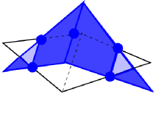
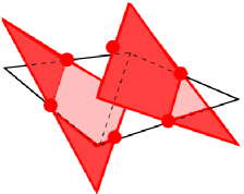
Figure 1: Basis functions (associated to an edge) for the Crouziex Raviart space (left figure) and the $\mathcal{Z}$ space (right figure)

A key property satisfied by the space decomposition (25) is that the two subpaces are orthogonal in the enegy norm defined by $\mathcal{A}_{0}(\cdot,\cdot)$. In fact it can be easily shown using (21) and the definition of the spaces (23) and (24) that

$$\mathcal{A}_{0}(v,z)=\mathcal{A}_{0}(z,v)=0\qquad\forall\,v\in V^{CR}\;,\,\,z\in\mathcal{Z}\;.$$ (26)

This already suggest that by perfoming a change of basis of the standard Lagrange basis for $V^{DG}$ to the ones in $V^{CR}$ and $\mathcal{Z}$, the stiffness matrix representation of $\mathbb{A}_{0}$ in the new basis have a block diagonal structure. Therefore, for the IP-0 method the following algorithm is an exact solver:

Algorithm 1: Let $u_{0}$ be a given initial guess. For $k\geq 0$, and given $u_{k}=z_{k}+v_{k}$, the next iterate $u_{k+1}=z_{k+1}+v_{k+1}$ is defined via the two steps:

1. Solve $\mathcal{A}_{0}(z_{k+1},\psi^{z})=(f,\psi^{z})_{\mathcal{T}_{h}}\quad\forall\,\psi^{z}\in\mathcal{Z}$.

2. Solve $\mathcal{A}_{0}(v_{k+1},\varphi)=(f,\varphi)_{\mathcal{T}_{h}}\quad\forall\,\varphi\in V^{CR}$.

Notice that algorithm 1 requires two solutions of smaller problems: one solution in $\mathcal{Z}$-space (step $1$ of the algorithm 1), and one solution in $V^{CR}$-space (step $2$ of algorithm 1). As we show next, the solution of the subproblems on $\mathcal{Z}$ and on $V^{CR}$ can be done efficiently.

Solution in the $\mathcal{Z}$-space: The functions in $\mathcal{Z}$ have non-zero jump on every edge, which suggest the high oscillatory nature of its functions. Using the definition of the space, the following useful property (Poincare-type inequality) can be shown:

Lemma 1

Let $\mathcal{Z}$ be the space defined in (24).

$$h^{-2}\|z\|_{0,\mathcal{T}_{h}}^{2}\lesssim\mathcal{A}_{0}(z,z)\lesssim h^{-2}\|z\|_{0,\mathcal{T}_{h}}^{2}\;,\qquad\forall\,z\in\mathcal{Z}$$

By virtue of this lemma it follows that the condition number (denoted by $\kappa$) of the block matrix associated to the restriction of $\mathcal{A}_{0}(\cdot,\cdot)$ to the subspace $\mathcal{Z}$, say $\mathbb{A}^{zz}_{0}$, satisfies $\kappa(\mathbb{A}_{0}^{zz})=O(1)$ and it is independent of the mesh size. Therefore, efficient solver for the problem in $\mathcal{Z}$ is the Conjugate Gradient (CG) method with a simple diagonal preconditioner.

Solution in $V^{CR}$: The restriction of $\mathcal{A}_{0}(\cdot,\cdot)$ to the $V^{CR}$ sub-space gives the well-known Crouziex-Raviart approximation method for (1) ;

$$\mathcal{A}_{0}(v,\varphi)=(\nabla v,\nabla\varphi)_{\mathcal{T}_{h}}=\sum_{T\in\mathcal{T}_{h}}(\nabla v,\nabla\varphi)_{T}\quad\forall\,\,v\,,\varphi\in V^{CR}\;,$$ (27)

Therefore, it is enough to resort to any of the solvers that have been already developed, for instance ayusob_plenary_brennerNC ; ayusob_plenary_Oswald96 ; ayusob_plenary_sarkisNC0 .

So far, an exact solver has been constructed in a simple and clean way for the IP-0 method. A last ingredient is needed to provide uniformly convergent solvers for the IP method (5) and it is formulated in next Lemma:

Lemma 2

Let $\mathcal{A}(\cdot,\cdot)$ and $\mathcal{A}_{0}(\cdot,\cdot)$ be the bilinear forms of the IIPG method defined in (5) and (21). Then, there exist $c_{2}>0$ depending only on the shape regularity of $\mathcal{T}_{h}$ and $c_{0}>0$ depending also on the penalty parameter $\alpha$ such that

$$c_{2}\mathcal{A}_{0}(u,u)\lesssim\mathcal{A}(u,u)\leq c_{0}\mathcal{A}_{0}(u,u)\quad\forall u\in V^{DG}.$$ (28)

The above result establishes the spectral equivalence between $\mathcal{A}_{0}(\cdot,\cdot)$ and $\mathcal{A}(\cdot,\cdot)$. Therefore, in terms of solution techniques, a uniform preconditioner for the IP-0 method, already provides a uniform preconditioner for the IP method.

These ideas and new framework, have been already extended and adapted for designing and analyzing solvers for other problems:

$\bullet$ In ayusob_plenary_jump the case of second order elliptic problems with large jumps in the diffusion coefficient is considered. In a first step, the space splitting (25) needs to be modified to account for the jumps in the coefficient, while still being orthogonal with respect to the corresponding $\mathcal{A}_{0}(\cdot,\cdot)$-induced norm. The choice of a robust method for approximating the continuous problem (definition of the relevant $\mathcal{A}(\cdot,\cdot)$ bilinear form) allows to guarantee that the corresponding spectral equivalence property (28) holds with constants $c_{0},c_{2}$ independent of the mesh size and the jumping coefficient.
$\bullet$ In ayusob_plenary_AyusoB_GeorgievI_KrausJ_ZikatanovL-2009aa efficient solvers are analyzed for IP approximations of linear elasticity problems, considering all cases: the pure displacement, the mixed and the traction free problems. The last two cases pose some extra pitfalls in the analysis since the spectral equivalence property (28) does not hold in those cases. In spite of that, the ideas can still be used to construct block preconditioners (guided by the algebraic structure of $\mathcal{A}_{0}(\cdot,\cdot)$ due to the orthogonality) and prove uniform convergence.
$\bullet$ In ayusob_plenary_ariel00 it is shown how to construct an efficient solver for the solution of the linear system that arise from a DG discretization of a convection-diffusion problem, in the convection dominated regime. The problem is relevant in semiconductor applications. In this case, the original method is a non-symmetric exponentially fitted IP weakly-penalized.

References

- (1) Antonietti, P., Ayuso de Dios, B., Bertoluzza, S., Penacchio, M.: BPS preconditioners for an hp Nitsche discretization. Tech. rep., IMATI-CNR, Pavia (17-PV-12/16/0) (2012). ArXiv:1301.3175
- (2) Antonietti, P.F., Ayuso, B.: Schwarz domain decomposition preconditioners for discontinuous Galerkin approximations of elliptic problems: non-overlapping case. Math. Model. Numer. Anal. 41(1), 21–54 (2007)
- (3) Antonietti, P.F., Ayuso, B.: Multiplicative Schwarz methods for discontinuous Galerkin approximations of elliptic problems. Math. Model. Numer. Anal. 42(3), 443–469 (2008)
- (4) Arnold, D.N.: An interior penalty finite element method with discontinuous elements. SIAM J. Numer. Anal. 19(4), 742–760 (1982)
- (5) Barker, A., Brenner, S., Park, E.H., Sung, L.: Two-level additive Schwarz preconditioners for a weakly over-penalized symmetric interior penalty method. J. Sci. Comput. (2010)
- (6) Brenner, S.C.: Two-level additive Schwarz preconditioners for nonconforming finite element methods. Math. Comp. 65(215), 897–921 (1996)
- (7) Brenner, S.C., Zhao, J.: Convergence of multigrid algorithms for interior penalty methods. Appl. Numer. Anal. Comput. Math. 2(1), 3–18 (2005)
- (8) Brezzi, F., Cockburn, B., Marini, L.D., Süli, E.: Stabilization mechanisms in discontinuous Galerkin finite element methods. Comput. Methods Appl. Mech. Engrg. 195(25-28), 3293–3310 (2006)
- (9) Brix, K., Campos Pinto, M., Canuto, C., Dahmen, W.: Multilevel preconditioning of discontinuous Galerkin spectral element methods. Part I: Geometrically conforming meshes. Tech. rep., IGPM Preprint, RWTH Aachen (2013). ArXiv:1301.6768
- (10) Brix, K., Campos Pinto, M., Dahmen, W.: A multilevel preconditioner for the interior penalty discontinuous Galerkin method. SIAM J. Numer. Anal. 46(5), 2742–2768 (2008)
- (11) Canuto, C., Pavarino, L., Pieri, A.: BDDC preconditioners for Continuous and Discontinuous Galerkin methods using spectral/hp elements with variable local polynomial degree. Tech. rep. (2012)
- (12) Ayuso de Dios, B., Georgiev, I., Kraus, J., Zikatanov, L.: Subspace correction methods for discontinuous Galerkin methods discretizations for linear elasticity equations. ESAIM: Math. Model. Numer. Anal. (2013). URL http://dx.doi.org/10.1051/m2an/2013070
- (13) Ayuso de Dios, B., Holst, M., Zhu, Y., Zikatanov, L.: Multilevel preconditioners for discontinuous Galerkin approximations of elliptic problems with jump coefficients. Math. Comp. (to appear)
- (14) Ayuso de Dios, B., Lombardi, A., Pietra, P., Zikatanov, L.: A block solver for the exponentially fitted IIPG-0 method. In: Twenty International Conference on Domain Decomposition, Lecture Notes in Computational Science and Engineering, vol. 91, pp. 247–255. Springer–Verlag (2013). URL http://dx.doi.org/10.1007/978-3-642-35275-1_28
- (15) Ayuso de Dios, B., Zikatanov, L.: Uniformly convergent iterative methods for discontinuous Galerkin discretizations. J. Sci. Comput. 40(1-3), 4–36 (2009)
- (16) Dobrev, V.A., Lazarov, R.D., Vassilevski, P.S., Zikatanov, L.T.: Two-level preconditioning of discontinuous Galerkin approximations of second-order elliptic equations. Numer. Linear Algebra Appl. 13(9), 753–770 (2006)
- (17) Dryja, M., Galvis, J., Sarkis, M.: BDDC methods for discontinuous Galerkin discretization of elliptic problems. J. Complexity 23(4-6), 715–739 (2007)
- (18) Dryja, M., Galvis, J., Sarkis, M.: Neumann-Neumann methods for a DG discretization of elliptic problems with discontinuous coefficients on geometrically nonconforming substructures. Numer. Methods Partial Differential Equations 28(4), 1194–1226 (2012)
- (19) Dryja, M., Sarkis, M.: FETI-DP method for a Composite Finite Element and Discontinuous Galerkin Method. SIAM J. Numer. Anal. 51(1), 400–422 (2013)
- (20) E. T. Chung, H.H.K., Widlund, O.B.: Two-level overlapping Schwarz algorithms for a staggered discontinuous Galerkin method. SIAM J. Numer. Anal. 51(1), 47–67 (2013)
- (21) Feng, X., Karakashian, O.A.: Two-level additive Schwarz methods for a discontinuous Galerkin approximation of second order elliptic problems. SIAM J. Numer. Anal. 39(4), 1343–1365 (electronic) (2001)
- (22) Gopalakrishnan, J., Kanschat, G.: A multilevel discontinuous Galerkin method. Numer. Math. 95(3), 527–550 (2003)
- (23) Hajian, S., Gardner, M.: Block Jacobi for discontinuous Galerkin discretizations: no ordinary Schwarz methods. Tech. rep. (2012). Submitted
- (24) Karakashian, O.A., Pascal, F.: A posteriori error estimates for a discontinuous Galerkin approximation of second-order elliptic problems. SIAM J. Numer. Anal. 41(6), 2374–2399 (electronic) (2003)
- (25) Lions, P.L.: On the Schwarz alternating method. I. In: First International Symposium on Domain Decomposition Methods for Partial Differential Equations (Paris, 1987), pp. 1–42. SIAM, Philadelphia, PA (1988)
- (26) Nepomnyaschikh, S.V.: Mesh theorems on traces, normalizations of function traces and their inversion. Soviet J. Numer. Anal. Math. Modelling 6(3), 223–242 (1991)
- (27) Oswald, P.: Preconditioners for nonconforming discretizations. Math. Comp. 65(215), 923–941 (1996)
- (28) Sarkis, M.: Nonstandard coarse spaces and Schwarz methods for elliptic problems with discontinuous coefficients using non-conforming elements. Numer. Math. 77(3), 383–406 (1997)
- (29) Schöberl, J., Lehrenfeld, C.: Domain decomposition preconditioning for high order hybrid discontinuous Galerkin methods on tetrahedral meshes. In: Advanced finite element methods and applications, Lect. Notes Appl. Comput. Mech., vol. 66, pp. 27–56. Springer (2013)
- (30) Toselli, A., Widlund, O.: Domain Decomposition Methods: Algorithms and Theory. Springer Series in Computational Mathematics (2005)
- (31) Widlund, O.B.: Some Schwarz methods for symmetric and nonsymmetric elliptic problems. In: Fifth International Symposium on Domain Decomposition Methods for Partial Differential Equations. SIAM (1992)
- (32) Xu, J.: Iterative methods by space decomposition and subspace correction. SIAM Rev. 34(4), 581–613 (1992)
- (33) Xu, J.: The auxiliary space method and optimal multigrid preconditioning techniques for unstructured grids. Computing 56(3), 215–235 (1996). International GAMM-Workshop on Multi-level Methods (Meisdorf, 1994)
- (34) Xu, J., Zikatanov, L.: The method of alternating projections and the method of subspace corrections in Hilbert space. J. Amer. Math. Soc. 15(3), 573–597 (2002)