Fine-scale Structures of Flux Ropes Tracked by Erupting Material

Abstract

We present the Solar Dynamics Observatory observations of two flux ropes respectively tracked out by material from a surge and a failed filament eruption on 2012 July 29 and August 04. For the first event, the interaction between the erupting surge and a loop-shaped filament in the east seems to “peel off” the filament and add bright mass into the flux rope body. The second event is associated with a C-class flare that occurs several minutes before the filament activation. The two flux ropes are respectively composed of 85$\pm$12 and 102$\pm$15 fine-scale structures, with an average width of about 1$\arcsec$.6. Our observations show that two extreme ends of the flux rope are rooted in the opposite polarity fields and each end is composed of multiple footpoints (FPs) of the fine-scale structures. The FPs of the fine-scale structures are located at network magnetic fields, with magnetic fluxes from 5.6$\times$10¹⁸ Mx to 8.6$\times$10¹⁹ Mx. Moreover, almost half of the FPs show converging motion of smaller magnetic structures over 10 hr before the appearance of the flux rope. By calculating the magnetic fields of the FPs, we deduce that the two flux ropes occupy at least 4.3$\times$10²⁰ Mx and 7.6$\times$10²⁰ Mx magnetic fluxes, respectively.

1 Introduction

The flux rope is thought to be closely related to the coronal mass ejection (CME), which generally has a three$-$part structure: the bright core, the dark cavity and the leading edge (see e.g., Illing & Hundhausen 1986). It is often believed that the twisted flux rope is the dark cavity which accumulates magnetic energy and mass within it (Chen 1996; Hudson & Schwenn 2000; Gibson et al. 2006). The ideal magnetohydrodynamic (MHD) instabilities of the flux rope such as the kink instability and the torus instability are thought to be one type of mechanism that triggers the CME and associated activities (Török & Kliem 2003, 2005; Fan 2005; Kliem & Török 2006; Olmedo & Zhang 2010). Thus, a detailed study of the flux rope is important for a clear understanding of CMEs, and this leads to a good ability to forecast CMEs and associated space weather.

The flux rope has been reconstructed in a complex magnetic topology from observed vector magnetograms by using non linear force-free field models (Guo et al. 2010; Canou & Amari 2010; Jing et al. 2010). Moreover, the formation and dynamic behavior of flux ropes have been simulated successfully by many authors (Amari & Luciani 1999; Amari et al. 2010; Fan & Gibson 2004). In the simulation of Aulanier et al. (2010), the flux rope is progressively formed by flux-cancellation-driven photospheric reconnection in a bald-patch separatrix.

Recently, the direct observations of flux ropes during the eruption process have been reported by using the data from the Atmospheric Imaging Assembly (AIA; Lemen et al. 2012) onboard the Solar Dynamics Observatory (SDO; Pesnell et al. 2012). Cheng et al. (2011) presented the observation of a flux rope as a bright blob of hot plasma in the channel of 131 Å. The hot flux rope rapidly moved outward and stretched the surrounding magnetic field upward, similar to the classical magnetic reconnection scenario in eruptive flares. Detailed thermal property of the flux rope based on differential emission measure was investigated by Cheng et al. (2012). However, there is to our knowledge no observations of fine-scale structures of flux ropes tracked by erupting material. In this letter, we present two events of flux ropes and investigate their fine-scale structures and magnetic properties by using the data from SDO/AIA and the Helioseismic and Magnetic Imager (HMI; Schou & Larson 2011).

2 Observations and Data Analysis

On 2012 July 29 and August 04, SDO/AIA observed two flux ropes that are respectively tracked by material from a surge and a failed filament eruption. Both of them are composed of thread-like structures, which warp and interweave together.

The SDO/AIA takes full-disk images in 10 (E)UV channels at 1$\arcsec$.5 resolution and high cadence of 12 s. The flux ropes could be observed in all the 7 EUV channels. The 171 channel best shows the flux rope and we focus on this channel in this study. We also present the observations of flux ropes in different channels such as 304, 193, 335 and 131 Å.

The 5 EUV channels correspond to different temperatures: 171 Å (Fe IX) at 0.6 MK, 304 Å (He II) at 0.05 MK, 193 Å (Fe XII) at 1.5 MK (with a hot contribution of Fe XXIV at 20 MK and cooler O V at 0.2 MK), 335 Å (Fe XVI) at 2.5 MK and 131 Å (Fe VIII, Fe XXI) at 11 MK (O’Dwyer et al. 2010; Boerner et al. 2012; Parenti et al. 2012). We also use the full-disk line-of-sight magnetic field data from the HMI onboard SDO, with a cadence of $\sim$ 45 s and a sampling of 0$\arcsec$.5 pixel^-1.

3 Results

3.1 Overview of the Two Flux Ropes

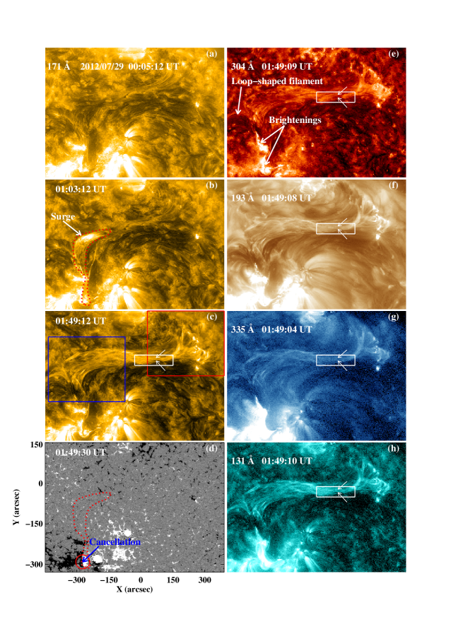
Figure 1: SDO$/$AIA multi-wavelength images and HMI line-of-sight magnetogram showing the evolution of the flux rope on 2012 July 29 (see Animations 1 and 2, available in the online edition of the journal). The red solid rectangle in panel c denotes the FOV of Figure 3a and the blue one denotes the FOV of Figure 3d.

At about 00:30 UT on 2012 July 29, a surge occurred in NOAA AR 11530 (S19W00) and plenty of material was ejected northward (see Figure 1b and Animation 1 in the online journal). By examining the SDO/HMI line-of-sight magnetograms, we found that the magnetic flux cancellation took place several hours prior to the surge (Figure 1d). The obvious brightening was observed at 171 Å at the location of the cancelled flux. This cancellation could be what led to the occurrence of the surge. When the surge first appears and starts to ascend, there is evidence of interaction between it and a loop-shaped filament in the east side of the erupting surge (see Figure 1e and Animation 2 in the online journal). This interaction seems to “peel off” the filament and to add mass into the flux rope body. Simultaneously, brightenings at the interaction location and the footpoint of the surge at 304 Å are also observed (see Figure 1e and Animation 2 in the online journal).

At about 00:52 UT, the erupting material seemed to be confined and moved toward the west (see Animation 1 in the online journal). Meanwhile, the bright fine-scale structures are clearly observed. About 52 min later (01:44 UT), the erupting material arrived at the west end of the flux rope and the entire flux rope was tracked out by the ejected material (see Figure 1c). It seems that the surge occurs within the flux rope and the footpoint of the surge is located at one end of the flux rope, and thus the material from the surge flows along the flux rope. The approximate length of the flux rope is 596 Mm, and the apparent flow speed of the material along the flux rope body is about 150 km s^-1. The flux ropes observed at 304, 193, 335 and 131 Å are roughly the same on the whole. However, they are different in some details. Taking the area denoted by white rectangles in Figure 1 for example, the 193 Å observations are similar to those of 171 Å, and the 304, 335 and 131 Å observations are different from 171 Å observations as the fine-scale structures (pointed by white arrows) are not clearly identified in these three channels.

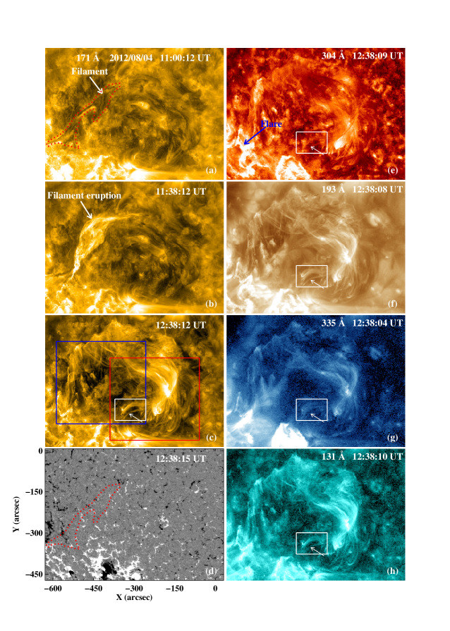
Figure 2: SDO$/$AIA multi-wavelength images and HMI line-of-sight magnetogram showing the evolution of the flux rope on 2012 August 04 (see Animations 3 and 4, available in the online edition of the journal). The red solid rectangle in panel c denotes the FOV of Figure 4a and the blue one denotes the FOV of Figure 4d.

On 2012 August 04, the second flux rope was observed in NOAA AR 11539 (S23E32). Before the flux rope was tracked, there existed a filament at the east part of the flux rope (see Figure 2a). At 11:04 UT, a C2.9 flare occurred at the east of the filament (see Figure 2e and Animation 4 in the online journal), which peaked at 11:47 UT and ended at 12:49 UT. At about 11:14 UT, the filament started to turn over and brighten (Figure 2b). At about 11:40 UT, the ejected material from the filament successively moved toward the southwest (see Animation 3 in the online journal). Then the arch-shaped flux rope with helical fine-scale structures was observed clearly (Figure 2c). The observed length of the flux rope is about 546 Mm, and it takes the filament material about 51 min to flow from the east to the west end. The apparent flow velocity along the flux rope body is approximately 180 km s^-1. Similar to the first flux rope on 2012 July 29, the fine-scale structures denoted by the white arrow in white rectangles of Figure 2 are identified clearly at 171 and 193 Å and seems obscure at 304, 335 and 131 Å. At about 16:00 UT on August 6, the east part of the second flux rope erupted, and this eruption resulted in a faint CME with a speed of about 260 km s^-1. The whole flux rope erupted at about 03:00 UT on August 8, associated with a halo CME with a speed of about 230 km s^-1.

3.2 Fine-scale Structures of the Two Flux Ropes

As the erupting material arrived at the west extreme end of the first flux rope on 2012 July 29, the west end showed obvious brightening (Figures 1c and 3a). Then partial material went back toward the east and brightened the east end at about 03:02 UT (see Figure 3d and Animation 1 in the online journal). The brightening at the ends makes it possible to determine the ends location. Thus we select two areas (denoted by red and blue rectangles in Figure 1c) to investigate the ends and fine-scale structures.

By counting the number of fine-scale structures one by one, we notice that the first flux rope is composed of 85$\pm$12 fine-scale structures, and 15 well identified fine-scale structures are selected to measure their widths. Two examples are shown in Figures 3c, f and g. Firstly, the intensity-location profiles (black curves in Figures 3f and g) along slices perpendicular to the fine-scale structures (Slices “S1” and “S2” in Figure 3c) are obtained. Secondly, we use Gaussian function to fit the intensity-location profiles and two Gaussian fitting profiles (blue and red ones) are shown in Figures 3f and g. The full width at half maximum (FWHW) of the Gaussian fitting profile is thought to be the width of fine-scale structure. The average width of these fine-scale structures is 1$\arcsec$.8, with the maximum value of 2$\arcsec$.0 and the minimum value of 1$\arcsec$.4.

For the first flux rope, there are 12 western footpoints (FPs) of the fine-scale structures that form the west end of the flux rope (white circles in Figure 3a). By comparing the 171 Å observations with line-of-sight magnetograms, we find that all the western FPs are rooted in negative polarity fields (Figure 3b). The net magnetic fluxes of these FPs are in the range of 8.6$\times$10¹⁸$-$8.6$\times$10¹⁹ Mx. The magnetic flux of the west end of the flux rope is $-$4.3$\times$10²⁰ Mx. This is the lower limit of the magnetic flux since some FPs are not identified and calculated for they are not accompanied by brightening. The 8 eastern FPs are rooted in positive polarity fields (Figures 3d and e). The net magnetic fluxes of eastern FPs are from 5.6$\times$10¹⁸ to 2.8$\times$10¹⁹ Mx. The magnetic flux of the east end of the flux rope is 1.3$\times$10²⁰ Mx, which is less than that of the western end. Not all the eastern FPs of the fine-scale structures are identified and thus there exists the discrepancy between the two sides.

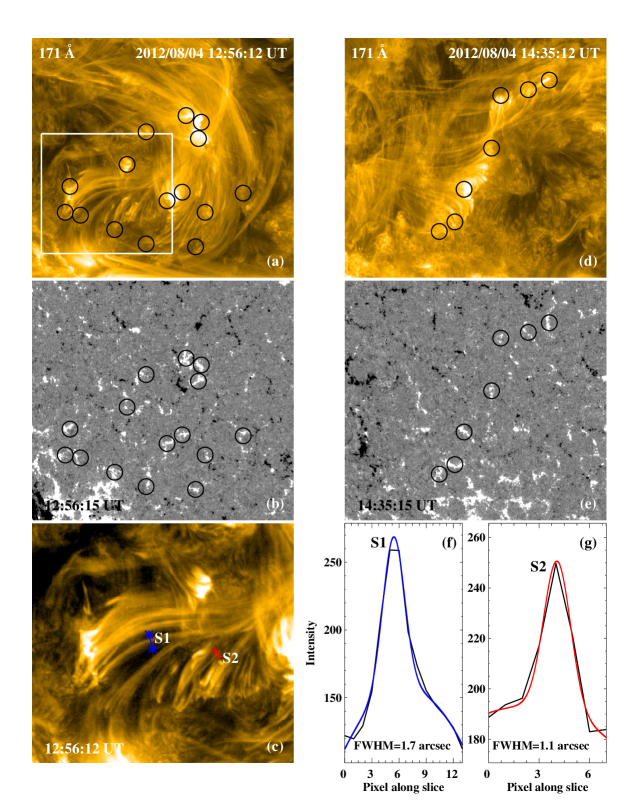
Figure 4: SDO$/$AIA 171 Å images and HMI magnetograms showing two main western ends of the flux rope (one in panels a$-$b and the other in panels d$-$e) on 2012 August 4, and the Gaussian fitting profiles (panels f and g) showing the widths of fine-scale structures. The white rectangle in panel a denotes the FOV of panel c.

For the second flux rope on 2012 August 04, we similarly select two areas where the brightening occurs at the ends (Figures 2c and 4). This arch-shaped flux rope seems more complex than the first one and has two main western ends (one in Figure 4a and the other one in Figure 4d) which are separated apart. The flux rope is composed of 102$\pm$15 fine-scale structures. The average width of 20 clearly identified fine-scale structures is 1$\arcsec$.5. The thickest one has a width of 1$\arcsec$.7, and the thinnest one has that of 1$\arcsec$.1 (Figures 4c, f and g). The line-of-sight magnetograms show that 22 western FPs (15 ones in Figures 4a$-$b and 7 ones in Figures 4d$-$e) of the fine-scale structures are anchored at positive polarity fields (Figures 4a$-$b, d$-$e). The net magnetic fluxes of these western FPs are in the range of 1.1$-$8.1$\times$10¹⁹ Mx. The total magnetic flux of western ends of the flux rope is 7.6$\times$10²⁰ Mx. The eastern end of the flux rope is close to the solar limb and not accompanied by EUV enhancements, thus it could not be identified.

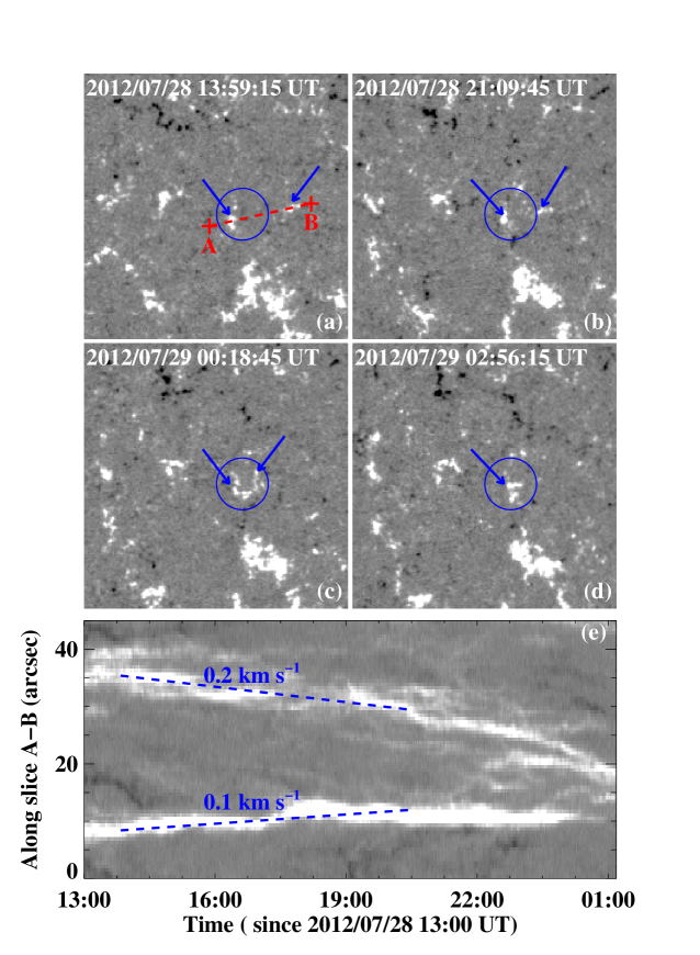
Figure 5: SDO$/$HMI magnetograms showing the converging motion of smaller magnetic structures at the FPs of the fine-scale structures. Blue circles denote one of the eastern FPs (“FP 1” in Figure 3e) of the fine-scale structures for the first flux rope on 2012 July 29. The stack plot along Slice “A$-$B” (red dashed line in panel a) is shown in panel e.

By examining the magnetic field evolution at the FPs of the fine-scale structures over 10 hr before the appearance of the flux rope, we find almost half of these FPs show converging motion of smaller magnetic structures for both the flux ropes. Figure 5 presents one example of the eastern FPs of the first flux rope. As seen in the stack plot along Slice “A$-$B”, the west magnetic structure obviously moved toward the east one with a velocity of 0.2 km s^-1 and the motion of the east one was slower than the west one, with a velocity of 0.1 km s^-1 (Figure 5e).

4 Summary and Discussion

We present the SDO/AIA observations of two flux ropes on 2012 July 29 and August 04 which are tracked out by material from a surge and a failed filament eruption. For the two flux ropes, the apparent speeds of filling of the flux rope structure with chromospheric and coronal plasma are respectively 150 and 180 km s^-1, which are comparable to the typical sound speed for the corona of about 100$-$200 km s^-1. For the first flux rope, the approximate length of the flux rope is 596 Mm. By examining the fine-scale structures which are observed more clearly, we roughly estimate the twist is about $\pi$. For event 2, the observed length of the flux rope is about 546 Mm, and the average twist is about 2$\pi$. Seen from the Solar-Terrestrial Relations Observatory (STEREO; Kaiser et al. 2008) B viewpoint, the two flux ropes are both located at the west limb. By using three-dimensional reconstructions, we obtain the heights of the two flux ropes, which are respectively 90 and 140 Mm above the solar surface. The two flux ropes analyzed here are respectively composed of 85$\pm$12 and 102$\pm$15 fine-scale structures, which probably outline the magnetic field structures of flux ropes (Martin et al. 2008; Lin 2011). The width of the fine-scale structures ranges from 1$\arcsec$.1 to 2$\arcsec$.0, with an average of about 1$\arcsec$.6. It is comparable to the resolution limit of the AIA telescope of about 1$\arcsec$.2, which suggests that even thinner structures may exist. Moreover, the width of the fine-scale structures is an order of magnitude larger than the ultrafine magnetic loop structures observed by Ji et al. (2012).

Before the flux ropes are tracked out by erupting material, part of magnetic flux rope structures may exist in the space filled in by the flux ropes. For event 1, there are several similar events in two days before the appearance of the first flux rope on 2012 July 29. Moreover, the 304 Å images shortly before the surge injection and flux rope appearance reveal the presence of long and thin absorbing threads along the first flux rope. For event 2, the filament at the east location of the flux rope may indicate part of the pre-existing flux rope structures.

When the surge in event 1 appears and the filament in event 2 is activated, the obvious brightenings and flare activities are observed simultaneously at the east of the two flux ropes. This implies that heating takes place and may illuminate the flux rope body by filling it with hot and dense plasma emitting in the EUV channels. This is similar to the observations of Raouafi (2009), who suggested that a C-class flare near one footpoint of the flux rope led to the brightening of the magnetic structure showing its fine structure. While the material arrives at the FPs of the fine-scale structures, the FPs are consequently brightened. The brightening at the FPs may be caused by the conversion from the kinetic energy to the thermal energy.

Our observations show that there exist 7$-$15 FPs of the fine-scale structures for each end of the flux rope. By comparing the EUV observations with the HMI magnetograms, we find that the FPs at one end of the flux rope on July 29 are rooted in the same polarity fields and the FPs at the other end are anchored at the opposite polarity fields (Figure 3). For the flux rope on August 04, the eastern end could not be identified and only the western end is analyzed here. The FPs of the fine-scale structures are located at network magnetic fields and their magnetic fluxes are in the range of 5.6$\times$10¹⁸$-$8.6$\times$10¹⁹ Mx. The magnetic fluxes of the two flux ropes are at least 4.3$\times$10²⁰ and 7.6$\times$10²⁰ Mx. According to the statistical study of Sung et al. (2009), the magnetic flux of 34 magnetic clouds (MC) for in-situ observations varies from 1.25$\times$10¹⁸ to 4.69$\times$10²¹ Mx with the average of 1.1$\times$10²¹Mx. The magnetic flux of the flux ropes in our observations is comparable to that of the MC. Moreover, almost half of the FPs of the fine-scale structures show converging motion of smaller magnetic structures over 10 hr before the appearance of the flux rope. The network magnetic field is often thought to be the converging center (Zhang et al. 1998), which is consistent with our observations. As small-scale magnetic fields located at the converging centers always exist tens of hours (Liu et al. 1994), implying that the flux ropes have a relatively long lifetime.

The flux ropes are observed in all the 7 EUV channels (304, 171, 193, 211, 335, 94 and 131 Å) of the SDO/AIA that cover the temperature from 0.05 MK to 11 MK. This is consistent with recent observations of Patsourakos et al. (2013) and Li & Zhang (2013), who reported the hot and cool components of flux ropes. However, there exist the flux ropes that could only be observed in hot channels such as 94 and 131 Å (Zhang et al. 2012; Cheng et al. 2011, 2012). The comprehensive characteristics of flux ropes need to be analyzed in further studies.

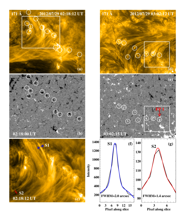
Figure 3: SDO$/$AIA 171 Å images and HMI magnetograms showing the western (panels a and b) and eastern ends (panels d and e) of the flux rope on 2012 July 29, and the Gaussian fitting profiles (panels f and g) showing the widths of fine-scale structures. The white rectangle in panel a denotes the FOV of panel c and white rectangles in panels d and e denote the FOV of Figure 5. The blue and red curves in panels f and g are respectively the Gaussian fitting profiles of the intensity-location curves (black ones) along the blue and red slices (Slices “S1” and “S2”) in panel c.

References

- (1) Amari, T., Aly, J.-J., Mikic, Z., & Linker, J. 2010, ApJ, 717, L26
- (2) Amari, T., & Luciani, J. F. 1999, ApJ, 515, L81
- (3) Aulanier, G., Török, T., Démoulin, P., & DeLuca, E. E. 2010, ApJ, 708, 314
- (4) Boerner, P., Edwards, C., Lemen, J., et al. 2012, Sol. Phys., 275, 41
- (5) Canou, A., & Amari, T. 2010, ApJ, 715, 1566
- (6) Chen, J. 1996, J. Geophys. Res., 101, 27499
- (7) Cheng, X., Zhang, J., Liu, Y., & Ding, M. D. 2011, ApJ, 732, L25
- (8) Cheng, X., Zhang, J., Saar, S. H., & Ding, M. D. 2012, ApJ, 761, 62
- (9) Fan, Y. 2005, ApJ, 630, 543
- (10) Fan, Y., & Gibson, S. E. 2004, ApJ, 609, 1123
- (11) Gibson, S. E., Foster, D., Burkepile, J., de Toma, G., & Stanger, A. 2006, ApJ, 641, 590
- (12) Guo, Y., Schmieder, B., Démoulin, P., et al. 2010, ApJ, 714, 343
- (13) Hudson, H., & Schwenn, R. 2000, Advances in Space Research, 25, 1859
- (14) Illing, R. M. E., & Hundhausen, A. J. 1986, J. Geophys. Res., 91, 1095
- (15) Ji, H., Cao, W., & Goode, P. R. 2012, ApJ, 750, L25
- (16) Jing, J., Yuan, Y., Wiegelmann, T., et al. 2010, ApJ, 719, L56
- (17) Kaiser, M. L., Kucera, T. A., Davila, J. M., St. Cyr, O. C., Guhathakurta, M., & Christian, E. 2008, Space Sci. Rev., 136, 5
- (18) Kliem, B., & Török, T. 2006, Physical Review Letters, 96, 255002
- (19) Li, L. & Zhang, J. 2013, A&A, 552, L11
- (20) Lin, Y. 2011, Space Sci. Rev., 158, 237
- (21) Liu, Y., Zhang, H., Ai, G., Wang, H., & Zirin, H. 1994, A&A, 283, 215
- (22) Lemen, J. R., Title, A. M., Akin, D. J., et al. 2012, Sol. Phys., 275, 17
- (23) Martin, S. F., Lin, Y., & Engvold, O. 2008, Sol. Phys., 250, 31
- (24) O’Dwyer, B., Del Zanna, G., Mason, H. E., Weber, M. A., & Tripathi, D. 2010, A&A, 521, A21
- (25) Olmedo, O., & Zhang, J. 2010, ApJ, 718, 433
- (26) Patsourakos, S., Vourlidas, A., & Stenborg, G. 2013, ApJ, 764, 125
- (27) Parenti, S., Schmieder, B., Heinzel, P., & Golub, L. 2012, ApJ, 754, 66
- (28) Pesnell, W. D., Thompson, B. J., & Chamberlin, P. C. 2012, Sol. Phys., 275, 3
- (29) Raouafi, N.-E. 2009, ApJ, 691, L128
- (30) Schou, J., & Larson, T. P. 2011, Bulletin of the American Astronomical Society, 1605
- (31) Sung, S.-K., Marubashi, K., Cho, K.-S., et al. 2009, ApJ, 699, 298
- (32) Török, T., & Kliem, B. 2003, A&A, 406, 1043
- (33) Török, T., & Kliem, B. 2005, ApJ, 630, L97
- (34) Zhang, J., Cheng, X., & Ding, M.-D. 2012, Nature Communications, 3, 747
- (35) Zhang, J., Wang, J., Wang, H., & Zirin, H. 1998, A&A, 335, 341