MOMENTUM DIFFUSION
OF ATOMS AND NANOPARTICLES
IN AN OPTICAL TRAP FORMED BY SEQUENCES
OF COUNTER-PROPAGATING LIGHT PULSES

Abstract

The motion of atoms and nanoparticles in a trap formed by sequences of counter-propagating light pulses has been analyzed. The atomic state is described by a wave function constructed with the use of the Monte Carlo method, whereas the atomic motion is considered in the framework of classical mechanics. The effects of the momentum diffusion associated with the spontaneous radiation emission by excited atoms and the pulsed character of the atom-to-field interaction on the motion of a trapped atom or nanoparticle are estimated. The motion of a trapped atom is shown to be slowed down for properly chosen parameters of the atom-to-field interaction, so that the atom oscillates around the antinodes of a non-stationary standing wave formed by counter-propagating light pulses at the point where they “collide”.

1 Introduction

Mechanical action of light on atoms [1,​ 2,​ 3,​ 4,​ 5,​ 6,​ 7,​ 8] is a cornerstone of modern atomic optics. In most cases, the required strengths of a light pressure are attained with the use of continuous laser radiation, which may be an additional factor that decreases the accuracy of physical experiments owing to light shifts induced by laser radiation. The control of the atomic motion with the help of light pulses can be a promising alternative, which would enable the interaction between the atom and the field to be so organized that the atom would be subjected to the action of laser radiation only within a short time intervals [9,​ 10,​ 11,​ 12,​ 13].

The optical trap for atoms proposed in work [9] is based of the interaction between atoms and sequences of counter-propagating $\pi$-pulses, which was studied in works [14,​ 15,​ 16] in detail. Figure 1 illustrates the mechanism of trap action. Let light pulses propagate along the $z$-axis. An atom at point $A$ has just undergone the action of pulse $R$ propagating from left to right, and soon it will be subjected to the action of pulse $L$ propagating from right to left. If this atom was in the ground state before the action of pulse $R$, the interaction with the latter transforms it into the excited state with the momentum $\hbar k$ directed along the $z$-axis. After being subjected to the action of pulse $L$, the atom emits a photon, and its momentum changes by another $\hbar k$ in the same direction. As a result of the interaction between the atom at point $A$ and a sequence of pulses that repeat with the period $T$, the atom is subjected to the action of the average force $2\hbar k/T$. A similar reasoning for an atom at point $B$ – in this case, the atom is first subjected to the action of pulse $L$ and, afterward, pulse $R$ – brings us to a conclusion that, owing to the interaction with a pair of counter-propagating pulses, its momentum changes by $-2\hbar k$, so that the average force acting on it equals $-2\hbar k/T$, i.e. directed toward point $C$. From the symmetry of the interaction between the atom and the field at point $C$, it follows that the force of light pressure on the atom equals zero. Hence, counter-propagating light $\pi$-pulses can form a trap for an atom. As was marked in works [9,​ 10], pulses with areas different from $\pi$ can also be used for this purpose.

The basic idea of the trap – invoking such a light pressure force that would act on the atom toward the point, where the counter-propagating pulses “collide” – was used in work [10] in order to focus a beam of atoms. The trap proposed in work [9] was theoretically analyzed in works [9,​ 12]. The authors of work [9] considered a variation of atom’s momentum and its scattering in the region of spatial overlapping between counter-propagating light pulses, when the atom interacts only once with them. The results obtained in the cited work are valid if two conditions are satisfied. First, the pulse repetition period should considerably exceed the lifetime of an atom in the excited state. Second, the atom must be in a state described by a wide wave packet, much wider than the wavelength of laser radiation. The authors of work [9] proposed the laser cooling in order to compensate the scattering-induced “heating” of atoms. In work [12], the force of light pressure averaged over an ensemble of slow atoms in such a trap was calculated for light pulses of an arbitrary area. Hence, the scattering of atoms in the region of spatial pulse overlapping, where the laser radiation field is close to a standing wave, was omitted from consideration.

The frequency detuning of monochromatic counter-propagating waves from the resonance with the frequency of an atomic transition is known [17,​ 18] to bring about the so-called Doppler cooling of the atomic ensemble, if the field frequency is lower than the transition one. The detuning magnitude should be close to the reciprocal lifetime of an atom in the excited state. In this case, the frequency of a transition in the atom, owing to the Doppler effect, is closer to the resonance with the counter-propagating wave, irrespective of the direction of atom’s motion, and the force of light pressure that slows down the atom exceeds the pressure force from the other wave that accelerates it. As a result, the atomic ensemble is cooled down. In work [19], it was demonstrated that atoms can also be cooled down in the field of counter-propagating pulses. Estimations of the light pressure force and the coefficient of momentum diffusion were made in work [19] for low-intensity fields, when they are equal to the sum of corresponding contributions made by counter-propagating waves. At the same time, for the analysis of the light trap in the field of counter-propagating pulses, high intensities of fields are optimal, when the areas of light pulses are close to $\pi$ and the force of light pressure cannot be considered as a sum of forces associated with each of the running sequences of counter-propagating pulses.

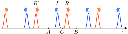
Fig. 1.: Interaction between an atom and sequences of counter-propagating pulses results in emerging a force that holds the atom near point C, where the pulses “collide”

In this work, we analyze the motion of an atom in a trap formed by light $\pi$-pulses. By examining the resonance interaction between the atom and the field, we shall estimate the influence of the momentum diffusion on atom’s motion in the trap. If the carrier frequency of light pulses is detuned from that of an atomic transition, a decelerating force emerges under certain conditions, and its influence can prevail over the influence of the momentum diffusion. As a result, the amplitude of atom’s oscillations in the trap becomes smaller than the wavelength. At the same time, owing to the momentum diffusion, the equilibrium position of the atom, around which it oscillates (at antinodes of the field), occasionally changes by half a wavelength. We did not manage to obtain analytical expressions for the description of this motion. Therefore, our research is based on the numerical simulation. To describe the evolution of the atomic state, we use a wave function constructed with the help of the Monte Carlo method [20]. Atom’s motion is described in the framework of classical mechanics, which corresponds to a narrow, in comparison with the wavelength, atomic wave packet.

In Section 2, the light fields that act on the atom are considered. The model shape of pulses, which is introduced there, is close to Gaussian-like, but is confined in time. In Section 3, we describe the Hamiltonian, which is used in Section 4 to construct the wave function with the use of the Monte Carlo method. Expressions for the calculation of the force and Newton’s equations needed for the description of atom’s motion are presented in Section 5. The procedure of numerical simulation of the state of atom and its motion is described in Section 6. Section 7 illustrates the application of the wave function constructed with the help of the Monte Carlo method to the description of a free, i.e. in the absence of the field, evolution of the atomic state. Here, the averaged elements of the density matrix for an ensemble of atoms are compared with the known analytical expressions. The results obtained at simulating the motion of atoms and nanoparticles in a trap formed by sequences of counter-propagating light pulses with the carrier frequency resonant with the frequency of a transition in the atom are reported in Section 8. In Section 9, we substantiate a possibility to keep atoms in the trap and, simultaneously, to cool them down by the same field. At last, in Section 10, the conclusions of the work are formulated in brief.

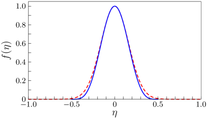
Fig. 2.: Comparison of the function $f(\eta)$ (see Eq. (4)) describing the envelope of light pulses (solid curve) and a Gaussian function that is the closest to it (dashed curve)

2 Light Pulses

Consider a two-level atom with the ground state $|1\rangle$, excited state $|2\rangle$, and the frequency of the transition between them $\omega_{0}$. The atom interacts with the field created by two counter-propagating sequences of pulses,

$$\bm{\mathrm{E}}(t)\!=\!E_{1}(t)\bm{\mathrm{e}}\cos[\omega{}t-kz+\varphi_{1}]\!+\!E_{2}(t)\bm{\mathrm{e}}\cos[\omega{}t\!+\!kz\!+\!\varphi_{2}].$$ (1)

Here, $E_{1,2}(t)$ are the pulse envelopes, $k=\omega/c$, $\mathbf{e}$ is the unit vector of polarization for the electric fields of pulses, $\varphi_{1}$ and $\varphi_{2}$ are the field phases at $t=0$ and $z=0$. To simplify the notations, the arguments for the field amplitudes, the density matrix elements, and the probability amplitudes will be omitted in most cases. We consider the interaction of an atom with a field created by two sequences of counter-propagating pulses with the repetition period $T.$ At the atom location point, one of the sequences repeats the other one with a certain time delay. The amplitudes of both pulses are described by the expression

$$E_{1{,}2}=E_{0}f(\eta_{1,2}){,}$$ (2)

where the function $f(\eta)$ with the maximum value $f(0)=1$ describes the shape of a pulse envelope,

$$\eta_{1{,}2}=(t\mp{}z/c)/\tau{,}$$ (3)

$z$ is the coordinate of the atom, and $\tau$ the pulse duration.

When the interaction between an atom and a field is simulated, the Gaussian-like pulses are usually applied [21,​ 22]. It is known [23,​ 16] that the function $\cos^{n}(\pi t/\tau)$ for large even $n$ tends to $\exp(-t^{2}/\tau_{\rm G}^{2})$ with $\tau_{\rm G}=\tau\sqrt{2}/(\pi\sqrt{n})$ within the interval $\left|t\right|<\tau/2$. Therefore, let us take $f(\eta)$ in the form

$$f(\eta)=\left\{\begin{array}[c]{ll}\cos^{4}(\pi{}\eta),&|\eta{}|<1/2,\\[2.84526pt] 0,&|\eta{}|>1/2.\end{array}\right.$$ (4)

In a vicinity of each pulse, this function is close to the Gaussian distribution

$$f_{\rm G}(\eta)=\exp\left(-2\pi^{2}\eta^{2}\right)$$ (5)

in the interval, where $f_{\rm G}(\eta)$ is not small (see Fig. 2).

In comparison with the Gaussian function (5), function (4) selected by us for the pulse simulation, on the one hand, is more convenient for numerical calculations (the Gaussian has to be artificially cut off beyond certain limits); on the other hand, it corresponds to real pulse envelopes restricted in time. The area of the pulse with the envelope described by function (4) equals $\frac{3}{8}\Omega_{0}\tau$ or approximately 0.94 times the area of the corresponding Gaussian pulse. The characteristic width of the latter equals $\tau_{\rm G}\approx 0.225\tau$.

3 Hamiltonian

Atom’s state will be described by a wave function constructed with the help of the Monte Carlo method [20]. After the averaging over the ensemble of realized atomic states, this approach becomes equivalent to the description of atom’s state using the density matrix. At the same time, in contrast to the latter, it allows an illustrative interpretation to be given for the evolution of the state of a separate atom. The Hamiltonian, which is used for the construction of such a wave function, differs from the Hamiltonian used in the equation for the density matrix by a relaxation term. It looks like

$${H}=H_{0}+H_{\mathrm{int}}+H_{\mathrm{rel}}{,}$$ (6)

where the term

$$H_{0}=\hbar\omega_{0}|2\rangle\langle 2|$$ (7)

describes the atom in the absence of the field and the relaxation. The term

$$H_{\mathrm{int}}=-\bm{\mathrm{d}}_{12}|1\rangle\langle 2|\bm{\mathrm{E}}(t)-\bm{\mathrm{d}}_{21}|2\rangle\langle 1|\bm{\mathrm{E}}(t){,}$$ (8)

where $\mathbf{d}_{12}$ is the matrix element of the electric dipole moment for the transition between states $|1\rangle$ and $|2\rangle$, which is responsible for the atom-to-field interaction, and the term

$$H_{\mathrm{rel}}=-\frac{i\hbar\gamma}{2}|2\rangle\langle{}2|$$ (9)

describes the relaxation owing to the spontaneous radiation emission. We emphasize that the relaxation component of Hamiltonian (6) looks like Eq. (9) if we describe atom’s state using the wave function constructed with the help of the Monte Carlo method. However, if we use the density matrix approach, the expression for $H_{\mathrm{rel}}$ is different [20].

4 Atomic Wave Function

The solution of the Schrödinger equation

$$i\hbar\frac{d}{dt}|\psi\rangle=H|\psi\rangle$$ (10)

is sought in the form

$$|\psi\rangle=c_{1}|1\rangle+c_{2}|2\rangle.$$ (11)

The substitution of Eq. (6) in Eq. (z10) gives us the following system of equations for $c_{1}$ and $c_{2}$:

$$\begin{array}[]{l}\displaystyle i\hbar\frac{d}{dt}c_{1}=-\bm{\mathrm{d}}_{12}\bm{\mathrm{E}}c_{2}{,}\\[14.22636pt] \displaystyle i\hbar\frac{d}{dt}c_{2}=\hbar\omega_{0}c_{2}-\bm{\mathrm{d}}_{21}\bm{\mathrm{E}}c_{1}-\frac{\gamma}{2}c_{2}.\!\!\!\!\!\!\!\!\\ \end{array}$$ (12)

For further calculations, it is convenient to separate a rapidly varying, with the frequency $\omega_{0}$, component in $c_{2}$. For this purpose, we make the substitutions $c_{1}=C_{1}$ and $c_{2}=C_{2}e^{-i\omega_{0}t}$. In the rotating wave approximation, i.e. when we neglect the rapidly oscillating terms including $e^{\pm 2i\omega_{0}t}$ in the equations for $C_{1}$ and $C_{2}$, Eq. (12) yields

$$\begin{array}[]{l}\displaystyle\frac{d}{dt}C_{1}=-\frac{i}{2}(\Omega_{1}e^{-ikz+i\Phi_{1}}+\Omega_{2}e^{ikz+i\Phi_{2}})C_{2}{,}\\[14.22636pt] \displaystyle\frac{d}{dt}C_{2}=-\frac{i}{2}(\Omega_{1}e^{ikz-i\Phi_{1}}\!+\!\Omega_{2}e^{-ikz-i\Phi_{2}})C_{1}\!-\!\frac{\gamma}{2}C_{2}{,}\!\!\!\!\!\!\!\!\\ \end{array}$$ (13)

where $\Omega_{1}=-\mathbf{d}_{12}\mathbf{e}E_{1}/\hbar$, $\Omega_{2}=-\mathbf{d}_{21}\mathbf{e}E_{1}/\hbar$, $\delta=\omega_{0}-$ $-\omega$, $\Phi_{1}=\varphi_{1}-\delta t$, and $\Phi_{2}=\varphi_{2}-\delta t$. Without loss of generality, the Rabi frequencies $\Omega_{1}$ and $\Omega_{2}$ may be considered to be real-valued quantities [24].

Hamiltonian (6) is non-Hermitian, and the squared absolute value of the wave function determined from the Schrödinger equation changes in time. In this connection, the procedure of function normalization should be carried out after every small step in time. In addition, the condition of a quantum jump within this time interval has to be testified [20].

Let us take a wave function $|\psi(t)\rangle$ normalized to 1 at the time moment $t$. The corresponding wave function $|\psi(t+\Delta{}t)\rangle$ at the time moment $t+\Delta t$ can be found in two stages, as is described below [20].

1. From the Schrödinger equation (10), it follows that, after a small enough $\Delta t$, the wave function $|\psi(t)\rangle$ transforms into

$$|\psi^{(1)}(t+\Delta{}t)\rangle\!=\!\left(\!1-\frac{i\Delta{}t}{\hbar}{{H}}\!\right)\!|\psi(t)\rangle.$$ (14)

Since Hamiltonian (6) is non-Hermitian, $\psi^{(1)}(t+\Delta{}t)$ is not normalized to 1. The square of its norm equals

$$\langle\psi^{(1)}(t+\Delta{}t)|\psi^{(1)}(t+\Delta{}t)\rangle=1-\Delta{}P{,}$$ (15)

where

$$\Delta{}P=\frac{i\Delta{}t}{\hbar}\langle\psi(t)|H-H^{+}|\psi(t)\rangle=\gamma\Delta{}t|C_{2}|^{2}.$$ (16)

2. At the second stage, let us consider a possibility of the quantum jump. If the value of random variable $\epsilon$, which is uniformly distributed between zero and 1, is larger than $\Delta P$ – in most trials, it is the case, because $\Delta P\ll 1$ – the jump is ignored, and the wave function at the time moment $t+\Delta t$ is assumed to equal

$$|\psi(t+\Delta{}t)\rangle=|\psi^{(1)}(t+\Delta{}t)\rangle/\sqrt{1-\Delta{}P},$$

$$\Delta{}P<\epsilon.$$ (17)

However, if $\epsilon<\Delta P$, the jump takes place, and the atom goes into the state

$$|\psi(t+\Delta{}t)\rangle=|1\rangle,\quad\Delta{}P>\epsilon.$$ (18)

Now, let us apply this procedure to the case where the field does not act on the atom (during the time interval between the light pulses). Let the initial atom’s state be

$$|\psi(0)\rangle=C_{1}(0)|1\rangle+C_{2}(0)|2\rangle.$$ (19)

At $t\rightarrow\infty$, the atom changes to a state $|1\rangle$ with the probability equal to $|C_{1}(0)|^{2}$ with no photon emission or to $|C_{2}(0)|^{2}$ if a photon is emitted.

If no quantum jump occurs within the time interval $[0,t]$, it follows from the Schrödinger equation with the Hamiltonian

$${H}=H_{0}+H_{\rm rel}$$ (20)

that

$$\psi^{(1)}(t)=\exp\left(\!-\frac{i}{\hbar}\int\limits_{0}^{t}H\,dt^{\prime}\!\right)\psi(0)=$$

$$=C_{1}(0)|1\rangle+C_{2}(0)\exp\left(\!-i\omega_{0}t-\frac{\gamma}{2}t\!\right)|2\rangle.$$ (21)

Normalizing the function $\psi^{(1)}(t)$ to 1, we obtain

$$\psi(t)=C_{1}(t)|1\rangle+C_{2}(t)\exp\left(-i\omega_{0}t)\right)|2\rangle{,}$$ (22)

where

$$\begin{array}[]{l}\displaystyle C_{1}(t)=\frac{C_{1}(0)}{\sqrt{|C_{1}(0)|^{2}+|C_{2}(0)|^{2}\exp(-\gamma{}t)}}{,}\\[14.22636pt] \displaystyle C_{2}(t)=\frac{C_{2}(0)\exp\bigl{(}-\frac{1}{2}\gamma{}t\bigr{)}}{\sqrt{|C_{1}(0)|^{2}+|C_{2}(0)|^{2}\exp(-\gamma{}t)}}.\!\!\!\!\!\!\!\!\\ \end{array}$$ (23)

The dependence of the wave function on the parameter $\gamma$, which is inserted by the absence of spontaneous radiation emission within the time interval $t$, is not evident. In the absence of radiation emission, the wave function should seemingly be equal to

$$\psi(t)=C_{1}(0)|1\rangle+C_{2}(0)\exp(-i\omega_{0}t)|2\rangle.$$ (24)

In this case, the probability of radiation emission within the time interval $[\Delta t{,}2\Delta t]$ would be the same as within the time interval $[0{,}\Delta t]$. Moreover, this probability would be the same for every of the following time intervals $\Delta t$, because the population of the excited state, $|C_{2}(0)|^{2}$, remains identical, and the atom would ultimately emit a photon. However, this conclusion contradicts the circumstance that, if $C_{1}(0)\neq 0$, the atom is in the ground state with the probability equal to $|C_{1}(0)|^{2}$ and will not emit a photon at all [20]. At the same time, the indicated contradiction is absent for the wave function (22), i.e. the probability of photon emission falls down in the course of time and approaches zero.

The probability that there will be no quantum jump within the time interval $[0,t]$ equals [20]

$$P(t)=|C_{1}(0)|^{2}+|C_{2}(0)|^{2}\exp(-\gamma{}t){}$$ (25)

and agrees with the probability of the absence of a quantum jump, $|C_{1}(0)|^{2}$, at $t\rightarrow\infty$ for the initial state (19) and with an exponential decrease of the excited state population in the ensemble of atoms.

Therefore, atom’s state at the time moment $t$ is described by the wave function (22) with the probability $P(t)$ or by the wave function

$$\psi(t)=|1\rangle$$ (26)

with the probability $1-P(t)$.

5 Atom’s Motion

Atom’s motion will be described in the framework of classical mechanics. During its interaction with light pulses, the atom undergoes the action of the force [1]

$$F=(\varrho_{12}\bm{\mathrm{d}}_{21}+\varrho_{21}\bm{\mathrm{d}}_{12})\frac{\partial\bm{\mathrm{E}}}{\partial z}{,}$$ (27)

where the density matrix elements are expressed in terms of $C_{1}$ and $C_{2}$ as follows:

$$\begin{array}[]{l}\displaystyle\varrho_{11}=|c_{1}|^{2}=|C_{1}|^{2}{,}\\[5.69054pt] \varrho_{22}=|c_{2}|^{2}=|C_{2}|^{2}{,}\\[5.69054pt] \varrho_{12}=c_{1}c_{2}^{*}=C_{1}C_{2}^{*}e^{i\omega_{0}{}t}{,}\\[5.69054pt] \varrho_{21}=c_{2}c_{1}^{*}=C_{2}C_{1}^{*}e^{-i\omega_{0}{}t}.\end{array}$$ (28)

After the averaging over the period of oscillations with the frequency $\omega_{0}$, the expression for force (27) in field (1) reads

$${F}=\hbar{}k\mathop{\mathrm{Im}}C_{1}C_{2}^{\ast}(\Omega_{1}e^{ikz-i\Phi_{1}}-\Omega_{2}e^{-ikz-i\Phi_{2}}).$$ (29)

The dependences of atom’s coordinate $z$ and velocity $v$ on the time are determined from the equations

$$\dot{v}=F/m{,}$$ (30)

$$\dot{z}=v{,}$$ (31)

where $m$ is atom’s mass.

Proceeding from the probability of a quantum jump equal to $1-P(t)$, where $P(t)$ between light pulses is determined by formula (25), we simulate the time moment of spontaneous radiation emission for every realization of the wave function. At this moment, atom’s coordinate does not change, and the projection of the momentum $\hbar\mathbf{k}$ transferred to the atom along the $z$-axis is determined, by assuming a random direction of light quantum emission.

6 Numerical Calculation Routine

To simulate the motion of atom, Eqs. (10), (30), and (31) were solved simultaneously. The time intervals, in which the atom interacts with the field, were divided into small subintervals, where the wave function was normalized and the presence of a quantum jump was checked. If so, atom’s velocity was modified according to the formula

$$\Delta{}v=\hbar{}k\cos(\pi\epsilon){,}$$ (32)

where $0<\epsilon<1$ is a random number with a uniform distribution over the interval $[0,1]$.

For the time intervals, when the field does not act on the atom, the wave function can be written down in an analytical form. Therefore, the calculation time can be considerably reduced, if, instead of simulating the quantum jump within numerous short time intervals during the free evolution of the atom, we will determine at once if there was a jump within the whole interval of free atom’s evolution and, if so, at which moment it happened. Let the atom after its interaction with the field be described by the wave function (19). The value of random variable $\epsilon$ should be compared with $|C_{1}(0)|^{2}$. The jump takes place if $\epsilon>|C_{1}(0)|^{2}$, and does not otherwise. Let us simulate the time moment of a quantum jump. We take another value for $\epsilon$ and calculate $\ln\epsilon$. For the exponential distribution of the probability

$$P_{e}=e^{-\gamma{}t}{,}$$ (33)

the quantity

$$t_{\mathrm{jump}}=-\left(\ln\epsilon\right)/\gamma$$ (34)

simulates the time moment, when the jump happens [25].

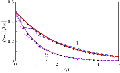
Fig. 3.: Comparison of the density matrix elements $\rho_{12}$ (curves 1) and $\rho_{22}$ (curves 2) calculated from the Monte Carlo wave functions (the dashed curves correspond to the averaging over 10 and the solid curves over 1000 realizations) with the exact expression (37) for the density matrix (circles). The initial conditions are $\rho_{12}(0)=1/2$, $\rho_{22}(0)=1/2$, and $|\psi(0)\rangle=\sqrt{2}\left[|1\rangle+|2\rangle\right]/2$

7 Example of Density Matrix Calculation Using the Wave Function Constructed with the Help of the Monte Carlo Method

Let us illustrate the equivalence between the descriptions of an atomic ensemble with the use of the wave function constructed with the help of the Monte Carlo method and the density matrix. Consider the free evolution of an atom, for which the variation of the density matrix in time can be easily calculated. The equation for the density matrix evolution looks like

$$\frac{d}{dt}\rho=i\omega_{0}[\rho,|2\rangle\langle{}2|]-$$

$$-\frac{\gamma}{2}\left(|2\rangle\langle{}2|\rho+\rho{}|2\rangle\langle{}2|\right)+\gamma{}|1\rangle\langle{}2|\rho{}|2\rangle\langle{}1|).$$ (35)

From whence, the equations for the density matrix elements follow,

$$\begin{array}[]{l}\displaystyle\frac{d}{dt}\rho_{22}=-\gamma\rho_{22},\\[14.22636pt] \displaystyle\frac{d}{dt}\rho_{12}=i\omega_{0}-\frac{\gamma}{2}{}\rho_{12},\\[14.22636pt] \displaystyle\rho_{21}=\rho_{12}^{*},\quad{}\rho_{11}=1-\rho_{22},\end{array}$$ (36)

and we obtain

$$\begin{array}[]{l}\displaystyle\rho_{22}(t)=\rho_{22}(0)\exp(-\gamma{}t),\\[14.22636pt] \displaystyle\rho_{12}(t)=\rho_{12}(0)\exp\left(\!i\omega_{0}t-\frac{1}{2}\gamma{}t\!\right)\!.\end{array}$$ (37)

The density matrix elements can also be calculated using the wave function constructed with the help of the Monte Carlo method, Eq. (28), and, afterward, carrying out the averaging over the ensemble of wave function realizations. Figure 3 testifies that the agreement between the density matrix elements calculated with the use of both approaches is satisfactory in the case of 10 wave function realizations and excellent in the case of 1000 ones.

Fig. 4.: Time evolution of intervals (between the upper and lower curves with identical numbers), in which the velocity (a) and the coordinate (b) of an atom with the mass $m=40\leavevmode\nobreak\ \mathrm{a.m.u.}$ in the trap created by the fields of counter-propagating $\pi$-pulses change. The pulse duration $\tau=1$ ps, the pulse repetition period $T=10$ ns, the carrier frequency of light pulses corresponds to a wavelength of 600 nm, and $\varphi_{1}=\varphi_{2}=0$. The parameter $\gamma=2\pi\times 10^{6}$ (1), $2\pi\times 10^{7}$ (2), and $2\pi\times 10^{8}\leavevmode\nobreak\ \mathrm{s}^{-1}$ (3). The initial conditions are $z=0$, and $v=0.2\leavevmode\nobreak\ \mathrm{m/s}$

8 Motion of Atoms and Nanoparticles in a Trap Formed by Sequences of Counter-Propagating $\pi$-Pulses

Consider atom’s motion in a trap formed by sequences of counter-propagating $\pi$-pulses. We suppose that the field frequency is resonant with that of a transition in the atom, $\delta=0$. When explaining the mechanism of trap action, we proceeded from the assumption that the atom at point $A$ (see Fig. 1) is in the ground state. Then, the sequence of influences by pulses $R$ and $L$ results in a variation of its momentum by $2\hbar k$ toward the trap center, point $C$. It is true in most cases. Really, since the time interval between pulses $L$ and $R$ is much shorter than that between pulses $L$ and $R^{\prime}$, the probability of spontaneous radiation emission by the atom in the excited state is much higher in the latter case. As a result, the atom at point $A$ will predominantly be in the ground state, and the force of light pressure on it will be directed toward the trap center. However, if the atom goes into the ground state after the action of pulse $R$ owing to spontaneous radiation emission, pulse $L$ returns it back to the excited state, and, during some time before the spontaneous emission, the atom undergoes the action of the force directed from the trap center. This process, when the force changes its direction, gives rise to a momentum diffusion, i.e. a spread of the atomic distribution with respect to atomic momenta [15,​ 16].

It is evident that the momentum diffusion process substantially depends on the rate of spontaneous radiation emission $\gamma$. In particular, the smaller is the value of $\gamma T$, the larger number of pairs of light pulses change atom’s momentum in the direction from point $C$ before the spontaneous radiation event. The momentum diffusion is minimal at $\gamma T\gg 1$, when the atom in the excited state at point $A$ has enough time to go into the ground state before the arrival of pulse $R^{\prime}$. Figures 4 and 5 illustrate a reduction of the momentum diffusion effect with the growth of $\gamma T$. They exhibit the intervals of changes in the velocity and the coordinate with time for atoms with the masses $m=40$ and 200 a.m.u., respectively, and for various rates of spontaneous radiation emission by the atom in the excited state. The time dependences of the coordinate and the velocity themselves are not shown, because the atom oscillates between the upper and lower curves marked by the same number, and the oscillation period is so small (less than 0.2 ms for the dependences shown in the figures) that the curves describing those dependences would entirely fill the space between the limits indicated in the figures.

At $\gamma T<1$, the time dependences of the interval, in which atom’s velocity varies (curves 1 and 2 in Figs. 4 and 5), only vaguely resemble the root one, which is typical of diffusion processes. The earlier researches [15,​ 16] of the momentum diffusion in the field of counter-propagating $\pi$-pulses and for a fixed delay between the pulses showed that the momentum diffusion coefficient

$$D=\frac{1}{2}\lim\limits_{t\rightarrow\infty}\frac{\langle{}p^{2}\rangle-\langle{}p\rangle^{2}}{t},$$ (38)

where $p$ is atom’s momentum, and the notation $\left\langle\ldots\right\rangle$ means the averaging over the ensemble, is approximately proportional to the delay between counter-propagating pulses. In our case, when the atom moves near the point, where those pulses “collide”, this delay is proportional to the atomic coordinate that changes in time. Hence, a simple analytical expression for $D$ obtained in work [15] is unsuitable in our case, and we can judge the character of diffusion-induced variations in the atomic momentum only on the basis of numerical calculations.

When the quantity $\gamma T$ increases above 1 (curves 3), the atom, owing to a high probability of its relaxation between pairs of counter-propagating pulses that are close in time, is practically always in the ground state before its interaction with the field.  This case was analyzed in work [9] for a one-time interaction between the atom and the field of a pulse pair, when the width of an atomic wave packet is wide in comparison with the wavelength of laser radiation.  In the region where counter-propagating pulses overlap, the field is close to that of a standing wave, and the diffraction of a wave packet takes place, which results in a spreading of the atomic distribution with respect to atomic momenta.  If the atomic wave packet is narrow in comparison with the wavelength of laser radiation, which corresponds to the classical description of atom’s motion, the distribution spreading over atomic momenta occurs owing to the pulsed atom-to-field interaction in the region, where the light pulses spatially overlap–the momentum transferred to the atom is determined by its relative coordinate with respect to the maxima and the minima of the field formed by counter-propagating laser pulses.  The atom does not move periodically in the field.  Therefore, when crossing the region where the light pulses overlap, it interacts every time with the field at a different point and, accordingly, obtains different momenta from the field. As a result, the character of its momentum change approaches the chaotic one (see curves 3 in Figs. 4 and 5).  Certainly, this mechanism of interaction between the atom and the field is valid in the case $\gamma T\ll 1$ as well, but the momentum variation owing to a change of the force direction after the event of spontaneous radiation emission dominates here.

When comparing Figs. 4 and 5, one can see that, under identical initial conditions, the oscillation limits of both the velocity and the coordinate get rapidly narrower for heavier atoms.  This fact is associated with a reduction of atom’s velocity variation $v_{r}=\hbar k/m=h/(\lambda m)$, where $\lambda$ is the wavelength of laser radiation, when absorbing or emitting a photon ($v_{r}=1.7\leavevmode\nobreak\ \mathrm{cm/s}$ for $m=40\leavevmode\nobreak\ \mathrm{a.m.u.}$ and 3.3 mm/s for $m=200\leavevmode\nobreak\ \mathrm{a.m.u.}$), which is analogous to a reduction of the diffusion coefficient in a gas for shorter mean free paths.

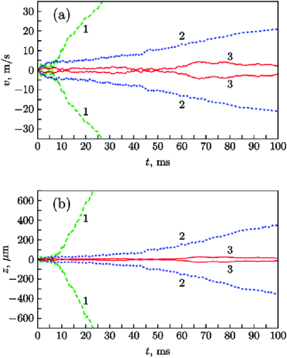
Fig. 5.: The same as in Fig. 4, but for an atom with the mass $m=200\leavevmode\nobreak\ \mathrm{a.m.u.}$

Hence, the trap created on the basis of counter-propagating light pulses possesses better properties for holding the heavy atoms – probably, with an additional cooling field [9] – such as Rb, Cs, and Th. Pulses with a short duration in comparison with the period of their repetition weakly perturb the atomic state. This is important, e.g., for high-precision spectroscopic researches, in particular, for the implementation of the frequency standard based on the optical nuclear transition in thorium [26,​ 27]. The trap has even better prospects for holding the nanoparticles with a low content – e.g., 0.1% – of “active” atoms with the transition frequency close to the carrier frequency of laser pulses. Such nanoparticles behave as “heavy atoms” with the atomic masses equal to tens of thousands. Accordingly, the momentum diffusion for such nanoparticles should be slower; therefore, they can be held in the trap using no additional cooling field.

Figure 6 demonstrates the variation intervals for the velocity and the coordinate of a nanoparticle with the specific mass $m=30000\leavevmode\nobreak\ \mathrm{a.m.u.}$ per one “active” atom. The curves were plotted for various spontaneous radiation rates of an atom in the excited state. The $z$-axis is directed upward. One can see that the gravitation force practically does not affect the motion of a nanoparticle. Similarly to the atoms with the masses $m=40$ and 200$\leavevmode\nobreak\ \mathrm{a.m.u.}$, the momentum diffusion decreases with the growth of $\gamma T$. In the case of large $\gamma T$ (curves 3), the oscillation limits for the nanoparticles do not change in time, at least till 0.1 s, and the influence of the momentum diffusion on nanoparticle’s motion is weak even at $\gamma T\ll 1$ (curves 1 and 2). Since the rate of spontaneous radiation emission $\gamma$ is fixed in every specific case, the product $\gamma T$ can be changed as required by varying the pulse repetition sequence. In the calculations carried out for the parameters that correspond to Figs. 4 and 5, but at $T=10^{-7}\leavevmode\nobreak\ \mathrm{s}$, a considerable reduction of the diffusion influence on atoms’ motion was observed.

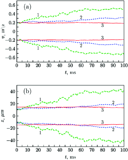
Fig. 6.: The same as in Fig. 4, but for a nanoparticle with the specific mass $m=30000\leavevmode\nobreak\ \mathrm{a.m.u.}$ per one “active” atom. The $z$-axis is directed vertically

Another controllable parameter, on which the interaction between the atom and the field depends, is a detuning of the light pulse carrier frequency from the frequency of the transition in the atom. In the next section, we shall demonstrate that even an insignificant, in comparison with the Rabi frequency, detuning of light pulses substantially modifies atom’s motion in the trap; in particular, it can suppress the momentum diffusion, provided a proper choice of other parameters.

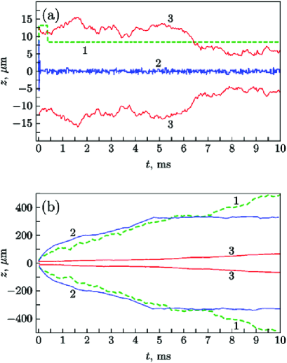
Fig. 7.: Time dependences of the coordinate and intervals of its changes (between the upper and lower curves with identical numbers) for an atom with the mass $m=200\leavevmode\nobreak\ \mathrm{a.m.u.}$ in the field of counter-propagating $\pi$-pulses. The pulse duration $\tau=1$ ps, the pulse repetition period $T=10$ ns, and $\varphi_{1}=\varphi_{2}=0$. The carrier frequency of light pulses corresponds to a wavelength of 600 nm and is detuned by $10^{10}\leavevmode\nobreak\ \mathrm{s}^{-1}$ below (a) and above (b) the transition frequency. The parameter $\gamma=2\pi\times 10^{6}$ (1), $2\pi\times 10^{7}$ (2), and $2\pi\times 10^{8}\leavevmode\nobreak\ \mathrm{s}^{-1}$ (3). The initial conditions are $z=0$, and $v=2\leavevmode\nobreak\ \mathrm{m/s}$

9 Atom’s Motion in a Trap Formed by Sequences of Counter-Propagating Pulses That Are Non-Resonant with the Transition Frequency in the Atom

Consider how the detuning of the laser radiation frequency from the resonance with the atomic transition frequency $\omega_{0}$ affects the interaction between the atom and the sequence of counter-propagating laser pulses. Figure 7 illustrates an example of the time dependence of the atomic coordinate (curves 1 and 2 in panel a) and shows the upper and lower coordinate limits, between which the atom oscillates (all other curves). One can see that, if $\delta>0$ (i.e. the carrier frequency of pulses is lower than the transition frequency in the atom) and $\gamma T<1$, the atom, after a short transient process, becomes localized in a narrow spatial interval. At $\gamma T>1$, the atom oscillates with a varying amplitude, by demonstrating a tendency to a reduction. This means that, if the atom is localized, the preservation of the coherent character of an atomic state within the pulse repetition period plays an essential role. On the other hand, at a low spontaneous radiation rate $\gamma=2\pi\times 10^{7}$ s^-1 (not shown in the figure), the amplitude of oscillations grows. This fact agrees well with the expression obtained in work [15] for the momentum diffusion coefficient in the case $\gamma T\ll 1$, namely, $D\sim 1/(\gamma T)$. Therefore, as the quantity $\gamma T$ decreases, the growth of the oscillation amplitude owing to the momentum diffusion should expectedly dominate over the atomic deceleration in the field of counter-propagating pulses.

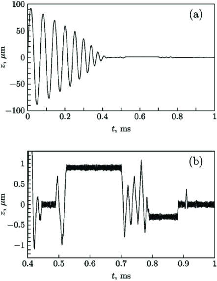
Fig. 8.: Time dependence of the coordinate for an atom with the mass $m=200\leavevmode\nobreak\ \mathrm{a.m.u.}$ in the field of counter-propagating $\pi$-pulses (a) and its scaled-up section (b). The pulse duration $\tau=1$ ps, the pulse repetition period $T=10$ ns, and $\varphi_{1}=$ $=\varphi_{2}=0$. The carrier frequency of light pulses corresponds to a wavelength of 600 nm and is by $10^{10}\leavevmode\nobreak\ \mathrm{s}^{-1}$ below the transition frequency. The rate of excited state damping $\gamma=2\pi\times 10^{7}\leavevmode\nobreak\ \mathrm{s}^{-1}$. The initial conditions are $z=0$, and $v=10\leavevmode\nobreak\ \mathrm{m/s}$

If the detuning sign changes (Fig. 7), the amplitude of atomic oscillations either grows (curves 1 and 3) or saturates (curve 2).

We made calculations for a number of other realizations of the Monte Carlo wave function, with other phases $\varphi_{1}$ and $\varphi_{2}$, and with a pulse area of $0.8\pi$ and obtained the time dependences of atom’s coordinate that are analogous to those exhibited in Fig. 7. The dependences of the same type were obtained for $\left|\delta\right|=10^{9}$ and $5\times 10^{10}$ s^-1. At the same time, for $\left|\delta\right|=10^{7}$, 10⁸, and $10^{11}$ s^-1, the decrease of atom’s velocity and its localization is observed at the opposite detuning, i.e. at $\delta<0$. The last result agrees with that obtained in work [19], where, as $\delta$ varied ($\delta>0$), the cooling of atoms is changed by their heating. If the detuning diminished to $\left|\delta\right|=10^{6}$ s^-1, no velocity reduction was observed for the parameters in Fig. 7. The results of numerical simulation of atom’s motion in the field of sequences of counter-propagating pulses brings us to a conclusion that a reduction of the amplitude and, accordingly, the velocity of atomic oscillations in the trap is possible in a wide interval of the field carrier frequency detuning from the resonance with the frequency of the atomic transition, provided the proper selection of $\delta$-sign. The pulse repetition period should be small enough for the condition $\gamma T<1$ to be satisfied.

Figure 8 illustrates the time dependence of the coordinate for parameters that provide the deceleration of an atom in the trap. At calculations, the initial velocity of the atom was selected to be much higher than that in Fig. 7. Owing to the interaction of the atom with light pulses, its velocity decreases from 10 to 0.2 m/s, which corresponds to the temperature change for an ensemble of 200-a.m.u. atoms with an initial root-mean-square velocity of 10 m/s from 2.4 K to 1 mK during 0.5 ms. The limiting temperature is a little higher that the Doppler cooling limit for atoms, $\hbar\gamma/k_{\rm B}\approx 0.4\leavevmode\nobreak\ \mathrm{mK}$, where $k_{\rm B}$ is the Boltzmann constant. Since the variation of the atomic velocity at the absorption or emission of a photon, $v_{\rm rec}=\hbar k/m$, equals approximately 0.003 m/s, at least 3000 photons were absorbed and emitted. As is seen from Fig. 8,b, the atom oscillates near the antinodes of a light wave, at a short distance from the coordinate origin, much shorter than the light pulse extension in the space (in particular, around $z=0$, $-\lambda/2$, $3\lambda/2$). At such distances from the coordinate origin, the fields of pulses from counter-propagating waves are almost identical. As a result, the atom is subjected to the action of a sequence of standing wave pulses, and cold atoms become captured at the corresponding antinodes. It is a well-known phenomenon that is observed in the stationary field of a monochromatic standing wave [3].

10 Conclusions

In this work, we have demonstrated that the momentum diffusion (a spread of the momentum distribution in an ensemble of atoms) in the resonance field of sequences of counter-propagating $\pi$-pulses or pulses close to them, which create a trap for atoms, depends substantially on the ratio between of the pulse repetition period and the time of spontaneous radiation emission.  At $\gamma T\sim 1$, the atom can be held in the trap for not less than 0.1 s.  While calculating the motion of nanoparticles in the trap under the condition $\gamma T\sim 1$, we did not observe the growth of the amplitude of their oscillatory motion around the trap center.

For a non-resonance field, we can made a selection of the detuning of light pulse carrier frequency and $\gamma T$ such that the amplitude of atom’s oscillations in the trap would considerably decrease, and the temperature in an ensemble of atoms could decrease almost to the Doppler cooling limit. As a result, the atoms become localized in vicinities of the antinodes of the non-stationary standing wave that is formed by counter-propagating light pulses in the region around the point of their “collision”. Since the field acts on the atom only during a short time interval, the pulse-created light trap can be used for high-precision spectroscopic researches. In particular, it can be used to hold atoms or ions of thorium-229, while developing the frequency standard on the basis of an optical nuclear transition [26,​ 27]. Another possible application of the trap on the basis of counter-propagating light pulses can be the manipulation with nanoparticles containing a small fraction of atoms (of about 0.1% or smaller) with the transition frequency close to the carrier frequency of light pulses.

The work was executed in the framework of the State goal-oriented scientific and engineering program “Nanotechnologies and Nanomaterials” (themes N 1.1.4.13 and 3.5.1.24).and sponsored by the State Fund for Fundamental Researches of Ukraine (project No. F40.2/039).

В.I. Романенко, О.В. Романенко,
О.Г. Удовицька, Л.П. Яценко
IМПУЛЬСНА ДИФУЗIЯ
АТОМIВ I НАНОЧАСТИНОК У ОПТИЧНIЙ
ПАСТЦI, УТВОРЕНIЙ ПОСЛIДОВНОСТЯМИ
ЗУСТРIЧНИХ СВIТЛОВИХ IМПУЛЬСIВ
Р е з ю м е
Розглянуто рух атомiв i наночастинок у пастцi, утворенiй послiдовностями зустрiчних свiтлових iмпульсiв. Стан атома описується хвильовою функцiєю, побудованою за допомогою методу Монте-Карло, його рух – класичною механiкою. Оцiнено вплив iмпульсної дифузiї, зумовленої спонтанним випромiнюванням збуджених атомiв та iмпульсним характером взаємодiї атома з полем, на рух атома чи наночастинки у пастцi. Показано, що при належно обраних параметрах взаємодiї атома з полем рух атома у пастцi гальмується, i вiн коливається бiля пучностей нестацiонарної стоячої хвилi, сформованої зустрiчними свiтловими iмпульсами поблизу точки, де вони ‘‘зiштовхуються’’.

References

- [1] V.G. Minogin and V.S. Letokhov, Laser Light Pressure on Atoms (Gordon and Breach, New York, 1987).
- [2] A.P. Kazantsev, G.I. Surdutovich, and V.P. Yakovlev, Mechanical Action of Light on Atoms (World Scientific, Singapore, 1990).
- [3] B.D. Pavlik, Cold and Ultracold Atoms (Naukova Dumka, Kiev, 1993) (in Russian).
- [4] H.J. Metcalf and P. van der Stratten, Laser Cooling and Trapping (Springer, Berlin, 1999).
- [5] S. Chu, Rev. Mod. Phys. 70, 685 (1998).
- [6] C.N. Cohen-Tannoudji, Rev. Mod. Phys. 70, 707 (1998).
- [7] W.D. Phillips, Rev. Mod. Phys. 70, 721 (1998).
- [8] V.I. Balykin, V.G. Minogin, and V.S. Letokhov, Rep. Prog. Phys. 63, 1429 (2000).
- [9] T.G.M. Freegarde, J. Waltz, and W. Hänsch, Opt. Commun. 117, 262 (1995).
- [10] A. Goepfert, I. Bloch, D. Haubrich, F. Lison, R. Schütze, R. Wynands, and D. Meshede, Phys. Rev. A 56, R3345 (1997).
- [11] V.I. Balykin, JETP Lett. 81, 206 (2005).
- [12] V.I. Romanenko and L.P. Yatsenko, J. Phys. B 44, 115305 (2011).
- [13] V.I. Romanenko and L.P. Yatsenko, Ukr. Fiz. Zh. 57, 893 (2012).
- [14] A.P. Kazantsev, Sov. Phys. JETP 39 784 (1974).
- [15] V.S. Voitsekhovich, M.V. Danileiko, A.M. Negriyko, V.I. Romanenko, L.P. Yatsenko, Zh. Èksp. Teor. Fiz. 99, 393 (1991).
- [16] A.M. Negriyko, V.I. Romanenko, and L.P. Yatsenko, Dynamics of Atoms and Molecules in Coherent Laser Fields (Naukova Dumka, Kyiv, 2008) (in Ukrainian).
- [17] V.S. Letokhov, V.G. Minogin, B.D. Pavlik, Opt. Commun. 19, 72 (1976).
- [18] V.S. Letokhov, V.G. Minogin, and B.D. Pavlik, Sov. Phys. JETP 45, 698 (1977).
- [19] K. Mølmer, Phys. Rev. Lett. 66, 2301 (1991).
- [20] C. Mølmer, Y. Castin, and J. Dalibard, J. Opt. Soc. Am. B 10, 524 (1993).
- [21] K. Bergmann, H. Theur, and B.W. Shore, Rev. Mod. Phys. 70, 1003 (1998).
- [22] N.V. Vitanov, T. Halfmann, B.W. Shore, and K. Bergmann, Annu. Rev. Phys. Chem. 52, 763 (2001).
- [23] V.I. Romanenko, Ukr. J. Phys. 51, 1054 (2006).
- [24] B.W. Shore, The Theory of Coherent Atomic Excitation, Vol. 1: Simple Atoms and Fields (Wiley, New York, 1990).
- [25] I.M. Sobol, The Monte Carlo Method (Univ. of Chicago Press, Chicago, IL, 1974).
- [26] E. Peik and Ch. Tamm, Europhys. Lett. 61, 181 (2003).
-
[27]
E. Peik, K. Zimmermann, M. Okhapkin, and Ch. Tamm, in
Proceedings of the 7th Symposium on Frequency Standards and
Metrology, edited by L. Maleki (World Scientific, Singapore, 2009),
p. 532.
Received 27.08.12.
Translated from Ukrainian by O.I. Voitenko