Quasi-Gasdynamic Approach for Numerical Solution of Magnetohydrodynamic Equations

Abstract

We introduce an application of the Quasi-Gasdynamic method for a solution of ideal magnetohydrodynamic equations in the modeling of compressible conductive gas flows. A time-averaging procedure is applied for all physical parameters in order to obtain the quasi-gas-dynamic system of equations for magnetohydrodynamics. Evolution of all physical variables is presented in an unsplit divergence form. Divergence-free evolution of the magnetic field is provided by using a constrained transport method based on Stokes theorem. Accuracy and convergence of this method are verified on a large set of standard 1D and 2D test cases.

1 Introduction

Up to now a variety of numerical methods to solve magnetohydrodynamic (MHD) equations is developed. Here we mention some of them, for example, Mac Cormack scheme (Yu et al., 2001), Lax-Friedrichs scheme (Tóth et al., 1996), the weighted essentially non-oscillatory scheme (WENO) (Jiang et al., 1999), piecewise parabolic method (PPM) (Dai et al., 1994) and its local variant PPML (Popov et al., 2008; Ustyugov et al., 2009). All of them are equipped by limiter functions for suppressing oscillations near discontinuities and approximate Riemann solvers (e.g. Roe (Brio, 1988), HLLC (Li, 2005) or HLLD (Miyoshi et al., 2005) solver). For practical applications a number of numerical codes have been developed up to now, for example for astrophycal simulations it should be mentioned Flash (Fryxell B. et al., 2000), Enzo (O’Shea B. et al., 2005), Athena (Stone et al., 2008) and Castro (Almgren et al., 2010).

An alternative approach for numerical modeling of MHD equations ia presented below. It can be regarded as generalization of regularized (or quasi-) gas dynamic (QGD) equation system suggested in last three decades, e.g.  (Chetverushkin, 2008; Elizarova, 2009; Sheretov, 2009).

The QGD equations are closely related to the Navier-Stokes (NS) equation system and can be written in the form of the NS system except for additional strongly non-linear terms. These additional terms contain the second-order space derivatives in a factor of a small parameter $\tau$ that has the dimension of time. These non-trivial $\tau$- terms bring an additional non-negative entropy production that proves their dissipative character and contribute to the stability of the numerical solution, e.g. (Elizarova, 2009; Sheretov, 2009). The $\tau$- terms depend on the solution itself and decrease in regions where space derivatives of the solution are small. In this sense the Quasi-Gasdynamic approach could be regarded as an approach with adaptive artificial viscosity.

Based on QGD equations, a family of finite-difference homogeneous schemes was constructed for numerical simulations of non-stationary gas flows. Efficiency, accuracy and simplicity of constructed algorithms are achieved due to regularization by $\tau$-terms, included in all equations of the system. The QGD schemes are constructed by applying central-difference approximation of all space derivatives, but due to the chosen $\tau$ form they have the space accuracy of the first order. The QGD algorithm differs from the other first-order finite-volume methods, and among its advantages the validity of the entropy theorem must be mentioned. The last feature is a critical point for mathematical description and numerical methods in fluid dynamics.

The applicability of the QGD algorithm was demonstrated in Elizarova et al. (2009), where stability and accuracy are studied numerically for ten classical Riemann test problems. The results revealed that the numerical solution monotonically converges to a self-similar one as the spatial grid is refined. Application of QGD algorithm for complex multidimensional gas-dynamical problems could be found in e.g. Elizarova et al. (2001); Mate et al. (2001); Graur et al. (2004); Chpoun et al. (2005). The QGD algorithms are well suitable for unstructured computational grids and are quite naturally generalized for the parallel realization using domain decomposition technique in order to speed up computation, e.g. Chetverushkin (2008).

In this paper, the extension of the QGD method is presented for a solution of magnetohydrodynamic (QMHD) equations in the numerical modeling of compressible heat-conducting gas. The QMHD system is obtained based on averaging of initial MHD system over small time interval and taking into account viscosity and thermal conductivity. Averaging in time is done for all physical parameters, including magnetic field as well, contrary to works  Sheretov (2009), where consideration of the magnetic field is taken mainly as an action of an external force. The first variants of the QMHD equations were obtained in 1997 together with calculations of electrically conductive liquid melt in external magnetic field, see citations in (Elizarova, 2009; Sheretov, 2009). As a result, correct computation is provided for complex cases of interaction with discontinuity of tangential component of the magnetic field. The QMHD algorithm was tested on a number of MHD problems in one-dimensional and two-dimensional cases. Among them the 2D Riemann problem for four states, blast wave propagation test, interaction of shock wave with a cloud and Orszag-Tang vortex problems are solved. The three last problems are also calculated in 3D formulation (Popov et al., 2013) and will be presented in details in further publication. The first results for 1D and 2D MHD calculations were published in Elizarova et al. (2011a) and Elizarova et al. (2011b) consequently.

Generalization of QMHD system for non-ideal gas together with the entropy theorem with nonnegative dissipative function has been performed in  (Ducomet et al., 2013). Here the influence of external forces and heat source are also included.

In the first section, the development of the quasi-gas-dynamic system of magnetohydrodynamic equation is presented. QMHD equations, numerical algorithm and finite-difference scheme are described in sections 3-4. Solenoidal condition for magnetic field is presented in section 4. Extensive testing of the QMHD scheme for one-dimensional and two-dimensional cases is discussed in section 5. In conclusion we stated about the possibilities of the QMHD scheme for flow simulations.

2 QMHD system of equations

The system of magnetohydrodynamic equations for viscous thermally conductive gas can be written in the following form:

$$\frac{\partial\rho}{\partial t}+\frac{\partial\rho u_{j}}{\partial x_{j}}=0,$$ (1)

$$\frac{\partial\rho u_{i}}{\partial t}+\frac{\partial T_{ij}}{\partial x_{j}}=0,$$ (2)

$$\frac{\partial E}{\partial t}+\frac{\partial Q_{j}}{\partial x_{j}}=0,$$ (3)

$$\frac{\partial B_{i}}{\partial t}+\frac{\partial T^{m}_{ij}}{\partial x_{j}}=0,$$ (4)

where

$$T_{ij}=\rho u_{i}u_{j}+p\delta_{ij}-\Pi_{ij}+\frac{1}{2}B^{2}\delta_{ij}-B_{i}B_{j},$$

$$Q_{j}=\rho u_{j}H-\Pi_{jk}u_{k}-q_{j}+u_{j}B^{2}-B_{j}\left(u_{k}B_{k}\right),$$

$$T^{m}_{ij}=u_{j}B_{i}-u_{i}B_{j},$$

$$E=\rho\varepsilon+\frac{\rho u^{2}}{2}+\frac{B^{2}}{2},\quad H=\frac{E+p}{\rho}$$

$$u^{2}=u^{2}_{x}+u^{2}_{y}+u^{2}_{z},\quad B^{2}=B^{2}_{x}+B^{2}_{y}+B^{2}_{z}.$$

Here $\rho$ is the density, $u_{i}$ is the velocity component, $B_{i}$ is the component of magnetic field, $E$ and $H$ are the total energy per unit volume, and total specific enthalpy respectively, $p$ is the pressure, $\varepsilon$ is the specific internal energy. The system of equations is supplemented by an equation of state, which in the case of ideal gas, has a form of

$$p=(\gamma-1)\,\rho\,\varepsilon,$$

where $\gamma$ is the adiabatic index.

Viscous stress tensor and heat-flux vector are defined as follows

$$\Pi_{ij}=\mu\left(\frac{\partial u_{i}}{\partial x_{j}}+\frac{\partial u_{j}}{\partial x_{i}}-\frac{2}{3}\delta_{ij}\frac{\partial u_{k}}{\partial x_{k}}\right),\\ \quad q_{i}=-k\frac{\partial T}{\partial x_{i}},$$

where $\mu$ is the dynamic viscosity coefficient,

$$k=\frac{\mu\gamma R}{(\gamma-1)Pr}$$ (5)

is the heat transfer coefficient, $Pr$ stands for the Prandtl number.

Implying the same approach as in  Elizarova (2011) we average the system (1)-(3) over a small time interval $\delta t$ and calculate the time integrals approximately as

$$\frac{1}{\delta t}\int_{t}^{t+\delta t}f(x_{i},t^{\prime})dt^{\prime}\approx f(x_{i},t)+\tau\frac{\partial f(x_{i},t)}{\partial t},$$

where $f$ denotes the averaging quantities. Here we assume that all include quantities have sufficient smoothness. We assume that $\delta t$ is smaller than the characteristic hydrodynamic time and that all averaged values practically do not depend on time interval $\delta t$ in some range of $\delta t$ (Sheretov, 2009; Elizarova, 2009). Parameter $\tau$ is small and related to interval of time averaging ($0\leq\tau\leq\delta t$), that is not strictly determined. So $\tau$ may be regarded as a free small parameter that will be precised later.

Then the system (1)-(3) could be rewritten as

$$\frac{\partial}{\partial t}\left(\rho+\tau\frac{\partial\rho}{\partial t}\right)+\frac{\partial}{\partial x_{j}}\left(\rho u_{j}+\tau\frac{\partial\rho u_{j}}{\partial t}\right)=0,$$

$$\frac{\partial}{\partial t}\left(\rho u_{i}+\tau\frac{\partial\rho u_{i}}{\partial t}\right)+\frac{\partial}{\partial x_{j}}\left(T_{ij}+\tau\frac{\partial T_{ij}}{\partial t}\right)=0,$$

$$\frac{\partial}{\partial t}\left(E+\tau\frac{\partial E}{\partial t}\right)+\frac{\partial}{\partial x_{j}}\left(Q_{j}+\tau\frac{\partial Q_{j}}{\partial t}\right)=0,$$

$$\frac{\partial}{\partial t}\left(B_{i}+\tau\frac{\partial B_{i}}{\partial t}\right)+\frac{\partial}{\partial x_{j}}\left(T^{m}_{ij}+\tau\frac{\partial T^{m}_{ij}}{\partial t}\right)=0.$$

Now we drop the terms of the form $\displaystyle{\frac{\partial}{\partial t}\tau\frac{\partial}{\partial t}}$ in time derivatives calculation supposing then they are small compared with the first-order time derivatives.

So, for example, the continuity equation writes as

$$\frac{\partial\rho}{\partial t}+\frac{\partial}{\partial x_{i}}\left(\rho u_{i}+\tau\frac{\partial}{\partial t}\rho u_{i}\right)=0.$$

Then we define the time derivative of momentum from the equation of motion

$$\frac{\partial\rho u_{i}}{\partial t}=-\frac{\partial}{\partial x_{j}}\left(\rho u_{i}u_{j}+p\delta_{ij}+\frac{1}{2}B^{2}\delta_{ij}-B_{i}B_{j}\right),$$

where we restrict our consideration with first-order terms only, i.e. omit values of the orders $O(\tau\mu)$. Introducing the definitions

$$w_{i}=\frac{\tau}{\rho}\frac{\partial}{\partial x_{j}}\left(\rho u_{i}u_{j}+p\delta_{ij}+\frac{1}{2}B^{2}\delta_{ij}-B_{i}B_{j}\right),\quad j_{mi}=\rho\left(u_{i}-w_{i}\right)$$

we present the continuity equation in smoothed form as follows:

$$\frac{\partial\rho}{\partial t}+\frac{\partial j_{mi}}{\partial x_{i}}=0.$$ (6)

In the same way, omitting the values of the order of $O(\tau k)$ we write the other equations of QMHD system as:

$$\frac{\partial\rho u_{i}}{\partial t}+\frac{\partial T_{ij}}{\partial x_{j}}=\frac{\partial\Pi^{n}_{ij}}{\partial x_{j}},$$ (7)

$$\frac{\partial E}{\partial t}+\frac{\partial F_{i}}{\partial x_{i}}+\frac{\partial Q^{n}_{i}}{\partial x_{i}}=\frac{\partial\Pi^{n}_{ij}u_{j}}{\partial x_{i}},$$ (8)

$$\frac{\partial B_{i}}{\partial t}+\frac{\partial T^{m}_{ij}}{\partial x_{j}}=-\frac{\partial T^{mn}_{ij}}{\partial x_{j}},$$ (9)

where

$$F_{i}=j_{mi}\left(H+\frac{B^{2}}{2\rho}\right)-B_{i}\left(u_{k}B_{k}\right),$$

$$T_{ij}=j_{mi}u_{j}+p\delta_{ij}+\frac{1}{2}B^{2}\delta_{ij}-B_{i}B_{j},$$

$$\Pi^{n}_{ij}=\Pi_{ij}-\rho u_{i}\Delta u_{j}-\Delta p\delta_{ij}-\frac{1}{2}\Delta B^{2}\delta_{ij}+\Delta\left(B_{i}B_{j}\right),$$

$$Q^{n}_{i}=q_{i}+\rho u_{i}\Delta\varepsilon+\rho u_{i}\left(p+B^{2}\right)\Delta\frac{1}{\rho}\\ +u_{i}\left(B_{k}\Delta B_{k}\right)-B_{i}\left(B_{k}\Delta u_{k}\right),$$

$$T^{mn}_{ij}=\Delta u_{j}B_{i}-\Delta u_{i}B_{j}+u_{j}\Delta B_{i}-u_{i}\Delta B_{j},$$

with $\tau$-terms presented using the definition $\tau\partial f/\partial t=\Delta f$. Here $\Delta$-terms are defined from the known magnetohydrodynamic equations

$$\Delta\frac{1}{\rho}=-\tau\left(u_{i}\frac{\partial}{\partial x_{i}}\frac{1}{\rho}-\frac{1}{\rho}\\ \frac{\partial u_{i}}{\partial x_{i}}\right),$$

$$\Delta u_{i}=-\tau\left(u_{j}\frac{\partial u_{i}}{\partial x_{j}}+\frac{1}{\rho}\frac{\partial p}{\partial x_{i}}\\ +\frac{1}{\rho}\frac{\partial}{\partial x_{j}}\frac{B^{2}}{2}\delta_{ij}\\ -\frac{1}{\rho}\frac{\partial B_{i}B_{j}}{\partial x_{j}}\right),$$

$$\Delta\varepsilon=-\tau\left(u_{i}\frac{\partial\varepsilon}{\partial x_{i}}+\frac{p}{\rho}\\ \frac{\partial u_{i}}{\partial x_{i}}\right),$$

$$\Delta p=-\tau\left(u_{i}\frac{\partial p}{\partial x_{i}}+\gamma p\\ \frac{\partial u_{i}}{\partial x_{i}}\right),$$

$$\Delta B_{i}=\tau\frac{\partial}{\partial x_{j}}\left(u_{i}B_{j}-u_{j}B_{i}\right).$$

The system (6)-(8) is the approximation of the initial system (1)-(3) with the order of $\tau$ and for $\tau=0$ equation system  (6)-(8) reduces to the classical system  (1)-(3). Notice, that the averaging procedure and the introducing of the $\tau$-terms do not disturb the solenoidal condition for the magnetic field ${\rm div}{\bf B}=0$.

3 Numerical algorithm

Let us introduce a uniform mesh for coordinates $x,y$ with steps $h_{x},h_{y}$, and time interval with step $\Delta t$. Values of all physical quantities, namely, the density, the velocity, the energy and the magnetic field are defined at the mesh nodes (cell centers). The flux values of all quantities are defined on the cell edges with semi-integer indices.

An explicit time-difference scheme of the following form is used to solve the derived system (6)-(8). For the density:

$$\overline{\rho}_{ij}=\rho_{ij}-\frac{\Delta t}{h_{x}}\left(j_{mi+1/2j}-j_{mi-1/2j}\right)-\\ \frac{\Delta t}{h_{y}}\left(j_{mij+1/2}-j_{mij-1/2}\right),$$

for the momentum components:

$$\overline{\rho u}_{k,ij}=\rho u_{k,ij}-\\ \frac{\Delta t}{h_{x}}\left(T^{n}_{k1,i+1/2j}-T^{n}_{k1,i-1/2j}\right)-\frac{\Delta t}{h_{y}}\left(T^{n}_{k2,ij+1/2}-T^{n}_{k2,ij-1/2}\right)+\\ \frac{\Delta t}{h_{x}}\left(\Pi^{n}_{k1,i+1/2j}-\Pi^{n}_{k1,i-1/2j}\right)+\frac{\Delta t}{h_{y}}\left(\Pi^{n}_{k2,ij+1/2}-\Pi^{n}_{k2,ij-1/2}\right),$$

for the total energy:

$$\overline{E}_{ij}\!=E_{ij}-\frac{\Delta t}{h_{x}}\!\left(F_{1,i+1/2j}\!-F_{1,i-1/2j}\right)-\frac{\Delta t}{h_{y}}\!\left(F_{2,ij+1/2}\!-F_{2,ij-1/2}\right)-\\ \frac{\Delta t}{h_{x}}\left(Q_{1,i+1/2j}-Q_{1,i-1/2j}\right)-\frac{\Delta t}{h_{y}}\left(Q_{2,ij+1/2}-Q_{2,ij-1/2}\right)+\\ \frac{\Delta t}{h_{x}}\!\left(\Pi^{n}_{1k}u_{k,i+1/2j}\!-\Pi^{n}_{1k}u_{k,i-1/2j}\right)+\frac{\Delta t}{h_{y}}\!\left(\Pi^{n}_{2k}u_{k,ij+1/2}\!-\Pi^{n}_{2k}u_{k,ij-1/2}\right).$$

To provide non-divergence of magnetic field we consider (9) in the form of Stokes’ theorem. The numerical algorithm to calculate the components of the magnetic field will be described in the next section.

The quantities with overbars here stand for the unknown values on a new time layer, which are computed via the known values on the previous time layer and the differences between the fluxes through the edges of the cell $(i,j)$. All quantities on the edges between cells are defined with simple averaging by adjacent cells, e.g. for the density as example it is

$$\rho_{i+1/2}=0.5\left(\rho_{i}+\rho_{i+1}\right).$$

We solve the system (6)-(8) in Euler approximation where the physical thermal conductivity and physical viscosity are neglected. All dissipative terms, containing $\mu$, $k$ and $\tau$ coefficients, are regarded as artificial regularization factors. The relaxation parameter and coefficients of the viscosity are linked and calculated as

$$\tau=\alpha\frac{h}{c_{f}},\quad\mu=\tau\cdot p\cdot Sc,$$ (10)

where $\alpha$ is the numerical coefficient to be taken in the range of $0.1-0.5$, $h=0.5\left(h_{x}+h_{y}\right)$. The Prandtl number and the Schmidt number could be set equal to one. The thermal conductivity is determined by (5). Coefficient $\alpha$ is chosen according with accuracy and stability of the numerical algorithm.

Note, that if we replace the step size $h$ by mean free path $\lambda$, then the expressions (10) with $\alpha=1$ exactly equal to expressions for a mean intercollisional time and mean free path in rarefied gases, obtained in kinetical theory, e.g., Bird (1994).

Time step $\Delta t$ is determined by the Courant condition

$$\Delta t=\beta\cdot min\left(\frac{h_{x}}{max_{ij}\left(|u_{x,ij}|+c_{fx,ij}\right)},\frac{h_{y}}{max_{ij}\left(|u_{y,ij}|+c_{fy,ij}\right)}\right),$$

where $\beta$ is the numerical Courant coefficient and in computations it falls in the range of $0.1-0.3$ in most cases, $c_{f}$ is the fast magnetosonic speed (Gardiner et al., 2005).

In the above numerical scheme all space derivatives are approximated by central differences, that provide the accuracy of order $O(h^{2})$. The definition of $\tau$ (10) decreases the accuracy down to $O(h)$. Formally, omitting the dependence $\tau\sim h$ and using high order central difference approximations one can increase the order of accuracy of the QMHD scheme. But resulting schemes will need special turning for $\tau$ value depending on the problem under consideration. For practical applications it is not convenient. Theoretical investigations and practical experience show, that for $\tau$ in form (10) with base values $\alpha=0.5$, $Sc=Pr=1$, QGD and QMHD algorithms uniformly describe a large variety of gas dynamic flows. In special cases tuning of numerical coefficients $\alpha$, $Sc$ and $Pr$ improves a numerical solution compared with base results (e.g. for Riemann problems in Elizarova et al. (2009), for MHD flows see test 5.4 below).

The QGD numerical scheme for non-uniform space grids could be constructed by replacing $h_{x}$ and $h_{y}$ for $h_{x,\,i}$ and $h_{y,\,j}$. Here the uniform space grids are presented for simplicity reason.

The presented numerical algorithm is simple because it is explicit, only central-difference approximations of the derivatives are used and additional monotonization procedures as limiting functions are not required.

4 Solenoidal condition for magnetic field

In the numerical solution of the QMHD system of equations, it is necessary to satisfy the solenoidal condition for the magnetic field (Tóth, 2000). For this purpose, Stokes’ theorem is used

$$\frac{\partial{\bf\,B}}{\partial\,t}=-\nabla\times{\bf E},$$

where the electric field is derived from formula $\bf E=-\bf u\times\bf B$, according to the MHD approximation. Components of the electric field are the corresponding components of the fluxes calculated through the edges of cells. Averaging these fluxes on adjacent cells, components of the electric field, defined on the edges of cells and required for the application of Stokes’ theorem, can be obtained. The method of this type was also implemented in e.g. Popov et al. (2008); Ustyugov et al. (2009).

In two-dimensional case, z-component of the electric field is required, determined at the nodes of the mesh as

$$E_{z,i+1/2j+1/2}=\frac{1}{4}\left(T_{21,i+1/2j}+T_{21,i+1/2j+1}\right.+\\ \left.T_{12,ij+1/2}+T_{12,i+1j+1/2}\right),$$

where $T_{ij}=T^{m}_{ij}+T^{mn}_{ij}$ includes $\tau$ regularizations. Using Stokes’ theorem, components of the magnetic field for the next time step are calculated as

$$B^{n+1}_{x,i+1/2j}=B^{n}_{x,i+1/2j}-\frac{\Delta t}{h_{y}}\left(E_{z,i+1/2j+1/2}-E_{z,i+1/2j-1/2}\right),$$

$$B^{n+1}_{y,ij+1/2}=B^{n}_{y,ij+1/2}+\frac{\Delta t}{h_{x}}\left(E_{z,i+1/2j+1/2}-E_{z,i-1/2j+1/2}\right).$$

Components of the magnetic field at the mesh center $\left(i,j\right)$ are obtained by half of the sum

$$B_{x,ij}=\frac{1}{2}\left(B_{x,i+1/2j}+B_{x,i-1/2j}\right),$$

$$B_{y,ij}=\frac{1}{2}\left(B_{y,ij+1/2}+B_{y,ij-1/2}\right).$$

Let us remark that for the solution of the QMHD system for three-dimensional case all three components of the magnetic field should be redefined.

5 Numerical tests

Described numerical scheme was verified on several distinctive one-dimensional and two-dimensional MHD problems to check its convergence and accuracy for Euler equations. For all tests, uniform mesh with constant step in each direction was set and equation of state of ideal gas was used. In one-dimensional case, all computations were performed on the interval $x\in[0\ldots 1]$. Initial values of vector $\bf V$ components, representing physical parameters, were defined on left and right sides from the middle point of the interval as following:

$${\bf V}=\left\{\begin{aligned} {\bf V}^{L},\quad\mbox{if}\ x\leq 0.5\,,\\ {\bf V}^{R},\quad\mbox{if}\ x>0.5\,.\\ \end{aligned}\right.$$

The number of numerical cells was equal to $N$, the final time for computations was notated as $T$. Boundary conditions were matched with corresponding initial conditions at the limits of the computational region. For every value $N$, we calculate relative error $\delta_{N}$ and the real order of accuracy $R_{N}$, using the following definitions:

$$\delta_{N}=\frac{1}{8}\sum^{i=8}_{i=1}E_{N}\left(V_{i}\right),$$

$$E_{N}\left(V_{i}\right)=\frac{\sum^{i=8}_{i=1}|V_{i,k}-V^{ex}_{i,k}|}{\sum^{i=8}_{i=1}|V^{ex}_{i,k}|},$$

$$R_{N}=log_{2}\left(\delta_{N/2}/\delta_{N}\right).$$

5.1 Riemann problem with initial discontinuity of transversal component of magnetic field

Initial conditions are given by Dai et al. (1994):

$$\left(\rho^{\,L},u^{\,L},v^{\,L},w^{\,L},B_{y}^{\,L},B_{z}^{\,L},p^{\,L}\right)=(1.0,0,0,0,1.0,0,1.0),$$

$$\left(\rho^{\,R},u^{\,R},v^{\,R},w^{\,R},B_{y}^{\,R},B_{z}^{\,R},p^{\,R}\right)=(0.125,0,0,0,-1.0,0,0.1).$$

Component of the magnetic field $B_{x}=0.75$, adiabatic index $\gamma=2$, $N=512$, $T=0.1$. The computational parameters are: Courant number $\beta=0.2$, regularization coefficient $\alpha=0.4$. Computation results are presented on Fig. 1-4. In this problem, the solution of the QMHD system of equations consists of fast rarefaction wave, moving to the left, intermediate shock wave and slow rarefaction wave, contact discontinuity, slow shock wave and one more fast rarefaction wave, moving to the right. The detailed discussion of this solution can be found in Jiang et al. (1999). On the figures, approximate solution is depicted by dots and exact solution is shown as solid line (it was obtained on the grid with $N=20000$ by the same code). Numerical scheme of QMHD system accurately represents all physical discontinuities and distribution behavior of all quantities without visible oscillations.

Notice, that similar pick in density and pressure distribution, as we see in Figs. 1 and. 2, are presented in many other computations of this problems performed by high order methods with limiters, see, e.g. Jiang et al. (2012); Popov et al. (2008).

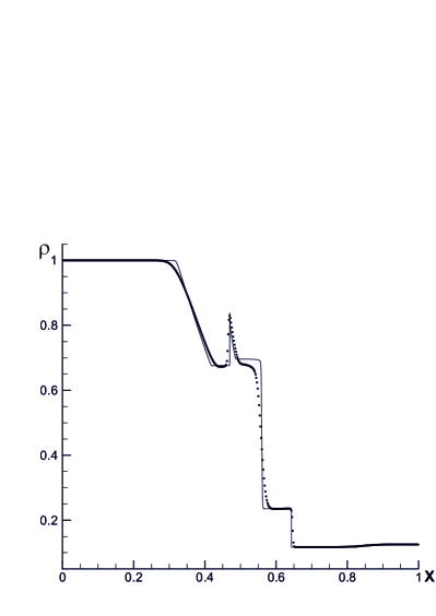
Figure 1: Test 5.1. Density distribution obtained on the grid $N=512$ in comparison with the exact one.

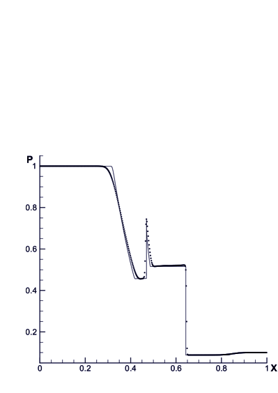
Figure 2: Test 5.1. The same for the pressure.

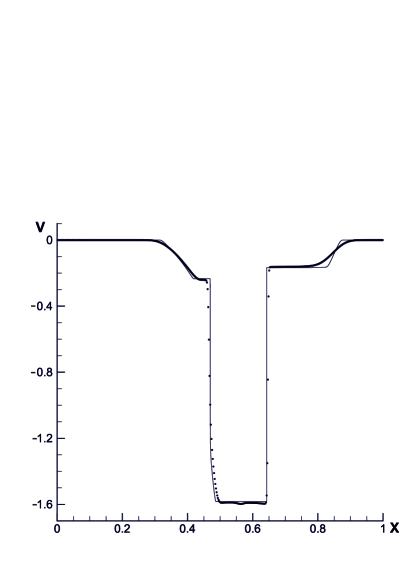
Figure 3: Test 5.1. The same for $y$-component of the velocity.

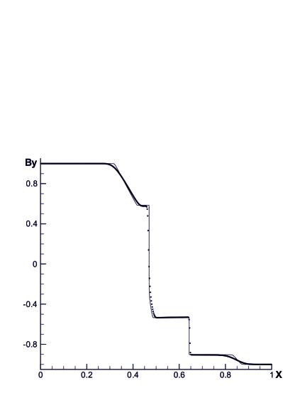
Figure 4: Test 5.1. The same for $y$-component of the magnetic field.

Table 1: Test 5.1. The average relative errors and the rates of convergence at $T=0.1$.

$N$	$\delta_{N}$	$R_{N}$
128	$6.91\times 10^{-2}$	-
256	$4.34\times 10^{-2}$	0.67
512	$2.74\times 10^{-2}$	0.67
1024	$1.52\times 10^{-2}$	0.85

As can be seen from Table 1, with mesh refinement the scheme error decreases with speed typical to first-order schemes. The quality of the numerical solution could be improved by adjustment of the numerical coefficients $Pr$ and $Sc$ (10) for this test case.

The same test was performed in Popov et al. (2008) using the PPML method that is third order-accurate in space and second order-accurate in time. The PPML results obtained on the grid with 512 cells are very similar to the presented above except the region of contact discontinuity. The PPML resolves contact discontinuities better but it requires more computational cost than QMHD. Still QMHD requires more detailed computational grid to obtain the comparative quality of a solution.

5.2 Riemann problem with formation of all forms of discontinuities

Here the solution consists of two fast shock waves with the speed equal to 1.84 and 1.28 of Mach number and directed to the left and to the right respectively, two slow shock waves, moving to the left and to the right with the speed 1.38 and 1.49 of Mach number correspondingly, one rotational and two contact discontinuities. Initial conditions are given by Dai et al. (1994):

$$\left(\rho^{\,L},u^{\,L},v^{\,L},w^{\,L},B_{y}^{\,L},B_{z}^{\,L},p^{\,L}\right)=\left(0.18405,3.8964,0.5361,\right.\\ \left.2.4866,2.394/\sqrt{4\pi},1.197/\sqrt{4\pi},0.3641\right),$$

$$\left(\rho^{\,R},u^{\,R},v^{\,R},w^{\,R},B_{y}^{\,R},B_{z}^{\,R},p^{\,R}\right)=\\ \left(0.1,-5.5,0,0,2/\sqrt{4\pi},1/\sqrt{4\pi},0.1\right).$$

Component of the magnetic field $B_{x}=4/\sqrt{4\pi}$, adiabatic index $\gamma=5/3$, $N=512,T=0.15$, Courant number $\beta=0.2$, regularization coefficient $\alpha=0.5$. Computation results are presented on Fig. 5-8.

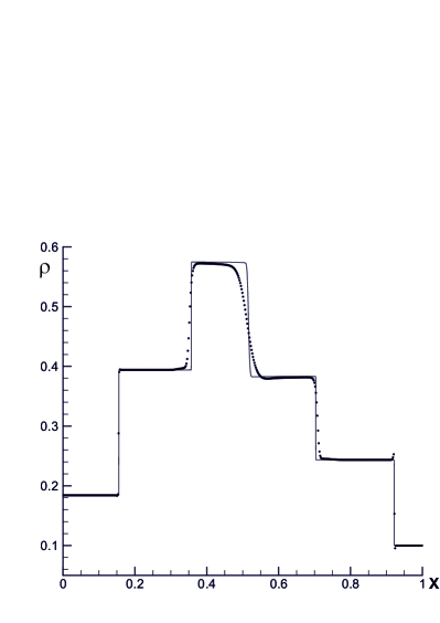
Figure 5: Test 5.2. Density distribution obtained on the grid $N=512$ in comparison with the exact one.

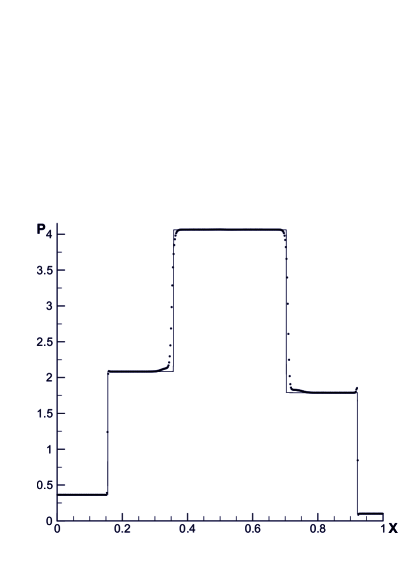
Figure 6: Test 5.2. The same for the pressure.

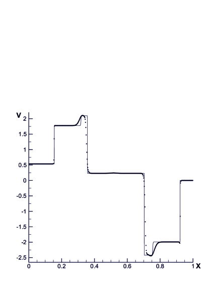
Figure 7: Test 5.2. The same for $y$-component of the velocity.

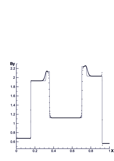
Figure 8: Test 5.2. The same for $y$-component of the magnetic field.

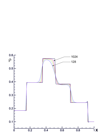
Figure 9: Test 5.2. Mesh convergence by example of the density. The computations were performed on the meshes from $N=128$ to $N=1024$ cells.

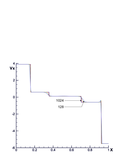
Figure 10: Test 5.2. The same for $x$ -component of the velocity.

Table 2: Test 5.2. The average relative errors and the rates of convergence at $T=0.15$.

$N$	$\delta_{N}$	$R_{N}$
128	$6.47\times 10^{-2}$	-
256	$3.65\times 10^{-2}$	0.83
512	$2.05\times 10^{-2}$	0.84
1024	$1.09\times 10^{-2}$	0.91

A solution convergence by consecutive reducing of mesh step by two times to exact solution of the problem for the density and the velocity profiles are shown on Fig. 9-10. Since the scheme has the first order of accuracy, it is implied from the computations that accurate enough distribution of the density is achieved on fine meshes, while the velocity and the pressure profiles are well resolved on rough meshes (Table 2).

5.3 Propagation of MHD waves in two-dimensional case

The next problem is a perfect quantitative test to determine accuracy and convergence order of a numerical algorithm. All physical parameters in entire computational domain are equal to constant values to be chosen that main waves are well enough distinct and the wave vector is directed at some angle to magnetic field. The waves are specified as perturbations to initial constant values of physical quantities in the following form

$$\delta{\bf U}=A{\bf R}\sin\left(2\pi x\right).$$

Here, $\bf U$ is the vector of conservative variables, $A$ is a magnitude, $\bf R$ is a vector of right eigenvectors of hyperbolic MHD system matrix with given numerical values for every wave. In all cases, the magnitude is $A=10^{-6}$. The size of computation domain is equal to the one wave length. Periodic boundary conditions are used for all variables. An error of numerical solution is measured by norm estimation after the wave once passes computational domain

$$||\delta{\bf U}||=\sqrt{\sum^{k=N}_{k=1}\left(\delta U_{k}\right)^{2}},\quad\delta U_{k}=\sum_{i}|U^{n}_{k,i}-U^{0}_{k,i}|/N,$$

Here, $U^{n}_{k,i}$ is a numerical solution for $k$-th component of vector of conservative variables for each point $i$ at the time moment $n$, $U^{0}_{k,i}$ is an initial solution and $N$ represents the number of points in the domain. Initial conditions are given by Sturrock (1994); Gardiner et al. (2005):

$$\rho=1,p=\frac{1}{\gamma},b_{x}=1,b_{y}=\sqrt{2},b_{z}=0.5,$$

where $b=B/\sqrt{4\pi}$ and $\gamma=5/3$.

The values of right eigenvectors components equal to:

for moving to the left fast magnetosonic wave

$${\bf R}=(0.4472135954999580,-0.8944271909999160,\\ 0.4216370213557840,0.1490711984999860,\\ 2.012457825664615,0.8432740427115680,\\ 0.2981423969999720),$$

for moving to the left Alfven wave

$${\bf R}=(0,0,-0.3333333333333333,\\ 0.9428090415820634,0,-0.3333333333333333,\\ 0.9428090415820634),$$

for moving to the left slow magnetosonic wave

$${\bf R}=(0.8944271909999159,-0.4472135954999579,\\ -0.8432740427115680,-0.2981423969999720,\\ 0.6708136850795449,-0.4216370213557841,\\ -0.1490711984999860),$$

where components of the right eigenvectors correspond to the ordering of the conservative parameters vector $\bf U$ of the form ${\bf U}=[\rho,v_{x},v_{y},v_{z},E,B_{y},B_{z}]$. Speed of the fast magnetosonic wave is equal to 2, the speed of Alfven wave is equal to 1 and the speed of slow magnetosonic wave is equal to 0.5. The absolute error in propagation of each of these waves and the order of numerical algorithm accuracy are presented in the following tables: for the fast magnetosonic wave (Table 3), for the Alfven wave (Table 4), for the slow magnetosonic wave (Table 5).

Table 3: Test 5.3. The average relative errors and the rates of convergence at $T=0.15$ for the fast magnetosonic wave.

$N$	$\delta_{N}$	$R_{N}$
64	$1.5395\times 10^{-7}$	-
128	$8.1368\times 10^{-8}$	0.9231
256	$4.1871\times 10^{-8}$	0.9618
512	$2.1243\times 10^{-8}$	0.9823
1024	$1.0700\times 10^{-8}$	0.9928
2048	$5.3696\times 10^{-9}$	0.9981

Table 4: Test 5.3. The average relative errors and the rates of convergence at $T=0.15$ for the Alfven wave.

$N$	$\delta_{N}$	$R_{N}$
64	$5.6148\times 10^{-8}$	-
128	$2.9196\times 10^{-8}$	0.9467
256	$1.4920\times 10^{-8}$	0.9718
512	$7.5461\times 10^{-9}$	0.9868
1024	$3.7953\times 10^{-9}$	0.9949
2048	$1.9033\times 10^{-9}$	0.9991

Table 5: Test 5.3. The average relative errors and the rates of convergence at $T=0.15$ for the slow magnetosonic wave.

$N$	$\delta_{N}$	$R_{N}$
64	$1.2508\times 10^{-7}$	-
128	$6.6601\times 10^{-8}$	0.9124
256	$3.4399\times 10^{-8}$	0.9564
512	$1.7485\times 10^{-8}$	0.9796
1024	$8.8157\times 10^{-9}$	0.9914
2048	$4.4262\times 10^{-9}$	0.9974

5.4 Numerical dissipation and decay of Alfven waves

In numerical modeling using a space mesh, any numerical scheme always has some dissipation. In order to estimate a level of numerical dissipation of the QMHD scheme a test on decay of Alfven waves was conducted (Balsara, 1998). At the initial moment of time, the Alfven wave has the following parameters

$$\delta u_{x}=u_{amp}c_{a}\sin\left(k_{x}x+k_{y}y\right),$$

and moves on fixed background with $\rho_{0}=1,p_{0}=1,B_{x}=1,B_{x}=B_{y}=0$.

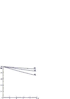
Figure 11: Test 5.4: Time evolution of the magnetic field $z$-component in computations on various meshes. Values of $N$ are represented by numbers.

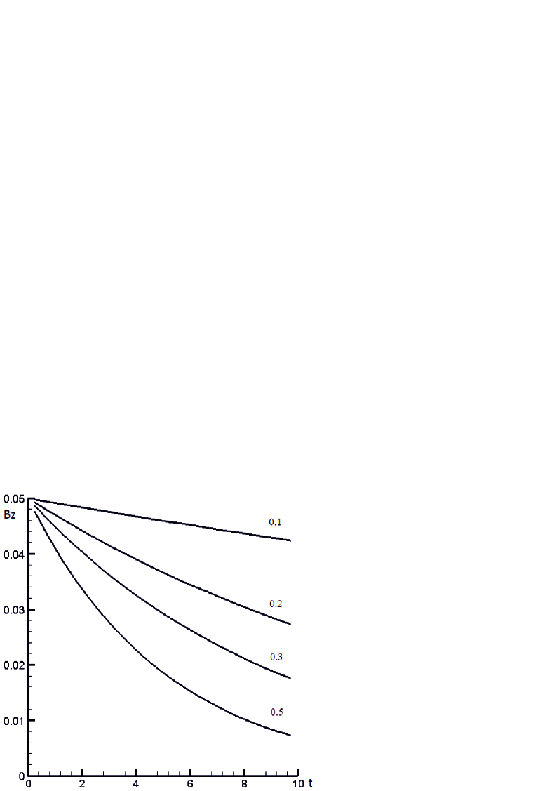
Figure 12: Test 5.4: The same on the mesh with $N=128$ at various values $\alpha$.

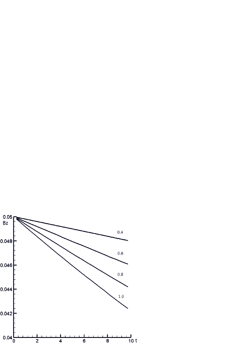
Figure 13: Test 5.4: The same at various Schmidt numbers $Sc$.

Computational domain represents a square of side $L=1$. Computations were performed on three meshes with number of cells in each direction $N=64$, $128$, $256$. The initial Alfven wave speed is $c_{a}=0.7071$ and its magnitude is $u_{amp}=0.1$, the adiabatic index is $\gamma=5/3$. Computations were done with the Courant number $\beta=0.3$, parameter $\alpha=0.1$ and with implementation of the periodic boundary conditions. Fig. 13 shows the time evolution of magnetic field $z$-component maximum on a sequence of twice refined meshes. Dissipation level corresponds to the schemes of the first order by space and time, and quickly decreases with mesh refinement. With the given Courant number and number of the mesh cells, Figs. 13-13 show that dissipation of the numerical scheme decreases with $\alpha$ and $S\!c$ parameters reducing.

The smallest dissipation level of the numerical scheme, wherein solution stability preserves, corresponds to values of parameters $\alpha=0.1$ and Schmidt number $S\!c=0.4$ on the mesh with $N=128$. In this case computational results are similar to results obtained with PPML method for $N=64$ (Popov et al., 2008; Ustyugov et al., 2009).

5.5 Propagation of a circularly polarized Alfven wave

This test problem was considered in the paper Gardiner et al. (2005) to study the accuracy and the order of convergence of numerical schemes on smooth solutions. The Alfven wave propagates along diagonal of the mesh at the angle $\theta=\tan^{-1}(0.5)\approx 26.6^{{\rm o}}$ to axis $x$. Computational domain has a size of $L_{x}=2L_{y}$, with cells number of $N_{x}=2N_{y}$. Since the wave does not move along diagonals of discrete cells, the problem has real multidimensional nature. Initial conditions are given by:

$$\rho=1,u_{||}=0,u_{\bot}=0.1\sin(2\pi\xi),u_{z}=0.1\cos(2\pi\xi),$$

$$p=1,B_{||}=0,B_{\bot}=0.1\sin(2\pi\xi),B_{z}=0.1\cos(2\pi\xi),$$

where $\xi=x\cos\theta+y\cos\theta$. Here, $u_{||},u_{\bot},B_{||},B_{\bot}$ are components of the velocity and the magnetic field, directed in parallel and perpendicular to the direction of the Alfven wave movement. The wave propagates towards a point $(x,y)=(0,0)$ with speed $B_{||}/\sqrt{\rho}=1$. The problem was solved with numerical cells of $N=16,32,64,128,256$ in the direction $x$, herewith relative numerical error was estimated for each quantity by the formula

$$\delta_{N}(U)=\frac{\sum^{i=2N}_{i=1}\sum^{i=2N}_{j=1}|U^{N}_{i,j}-U^{E}_{i,j}|}{\sum^{i=2N}_{i=1}\sum^{i=2N}_{j=1}|U^{E}_{i,j}|}\\ ,\quad U=u_{\bot},u_{z},B_{\bot},B_{z},$$

where $U^{E}_{i,j}$ is the exact solution. Convergence order of the scheme was estimated as

$$R_{N}=\log_{2}\left(\delta_{N/2}/\delta_{N}\right),$$

where $\delta_{N}$ was defined as mean by

$$\delta_{N}=\frac{1}{4}\left(\delta_{N}(u_{\bot})+\delta_{N}(u_{z})+\delta_{N}(B_{\bot})+\delta_{N}(B_{z})\right),$$

The computations were carried out until the time moment of $t=5$ with the Courant number of $\beta=0.2$ , the parameter $\alpha=0.1$, the adiabatic index $\gamma=5/3$, and with the periodic boundary conditions were used. On the Fig. 14, orthogonal component $B_{\bot}$ of the magnetic field is presented in computations on various meshes. The values of $N$ are indicated by numbers. It can be seen that the numerical solution of the problem tends to the exact solution with increasing of $N$. Obtained results confirm that with increasing of the resolution the numerical scheme has the first order of accuracy in space and time. The same test was performed by PPML code in Popov et al. (2008). For PPML method acceptable numerical solution begins from the grid resolution equal to 32 cells, but for QMHD – from 64 cells.

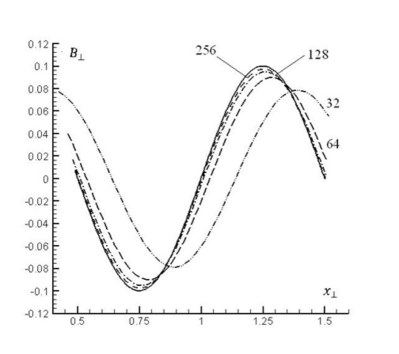
Figure 14: Test 5.5: The lines of orthogonal component of the magnetic field in the computations on various meshes. The values of N are indicated by numbers.

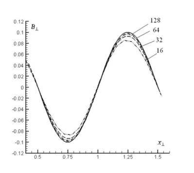
Figure 15: Test 5.5: The lines of the perpendicular component of the magnetic field in the computations on various meshes in the case of the stationary wave. The values of $N$ are indicated by numbers.

Also, computations were performed for the case of the stationary Alfven wave with $u_{||}=1$. On Fig. 15, the orthogonal component $B_{\bot}$ of the magnetic field are presented in computations on various meshes. The values of $N$ are indicated by numbers. In Table 6, the average relative error and the order of convergence are shown. It can be seen that the numerical solution of the problem with increasing of $N$ rapidly tends to the exact solution and the order of convergence is close to one even for small $N$. These results are compared with high-order Constrained Transport/Central Difference(CT/CD) scheme (Tóth, 2000), see Table 7. Comparison of the tables shows, that for $N=16$ the accuracy of both methods are similar, and for $N=32$ and 64 the accuracy of Flux-CD/CT scheme is approximately two times higher.

Table 6: Test 5.5. The average relative errors and the rates of convergence with $u_{||}=1$

$N$	$\delta_{N}$	$R_{N}$
16	0.12671	-
32	0.064888	0.9688
64	0.032914	0.9825
128	0.016569	0.9935
256	0.0083133	0.9984

Table 7: Test 5.5. The same for $u_{||}=1$ by Flux-CD/CT scheme taken from Tóth (2000).

$N$	$\delta_{N}$	$R_{N}$
8	$0.315$	-
16	$0.122$	1.368
32	$0.037$	1.721
64	$0.013$	1.509

5.6 A blast wave propagation through magnetized medium

In this problem, a propagation of the initial finite perturbation of the pressure through a medium with superimposed magnetic field (Dai et al., 1998) is investigated. The problem is solved in the square computational domain with side dimension $L=1$ and number of cells $400\times 400$. In the initial time, in the entire domain the initial density $\rho=1$ and pressure $p=1$, excepting central part with radius $r=0.05$, where pressure is $p=1000$. Uniform magnetic field with magnitude $B=10$ is directed along axis $x$. The adiabatic index $\gamma=1.4$. Computations were carried out until time $t=0.02$ with the Courant number $\beta=0.1$, the parameter $\alpha=0.4$. Gradients of all parameters were equal to zero on the domain boundary. Figs. 16-17 present the numerical solution at $t=0.02$.

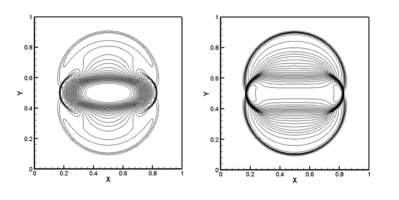
Figure 16: Test 5.6: Distribution of logarithm of the density and logarithm of the pressure.

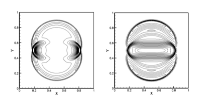
Figure 17: Test 5.6: Distribution of the kinetic energy and logarithm of the magnetic energy.

Magnetic field introduces anisotropy in a substance expansion. Under the action of the pressure, substance accelerates along magnetic field lines, and shock waves with higher kinetic and magnetic energy can be seen on the boundary in the middle part of the domain. A rarefied area with lower density and pressure and the prevalence of magnetic energy over the kinetic and thermal energy forms in the center of the square. In spite of the large initial difference in the pressure and high magnetization of the medium in the middle part of the computation domain, the numerical QMHD scheme provides positive values of the pressure and density, and describes all intrinsic discontinuities with good accuracy for the scheme of the first order in space and in time at the final stage of substance expansion.

5.7 Two-dimensional Riemann problem with four states with the magnetic field

Structures formation is studied in the interaction of the four states with a superimposed magnetic field (Dai et al., 1998; Arminjon et al., 2005). Initial conditions are given by:

$$(\rho,p,u_{x},u_{y}) =(1,1,0.75,0.5), x>0,y>0$$

$$(\rho,p,u_{x},u_{y}) =(2,1,0.75,0.5), x<0,y>0$$

$$(\rho,p,u_{x},u_{y}) =(1,1,-0.75,0.5), x<0,y<0$$

$$(\rho,p,u_{x},u_{y}) =(3,1,-0.75,-0.5), x>0,y<0$$

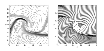
Figure 18: Test 5.7: Distributions of density contour lines and magnetic field lines.

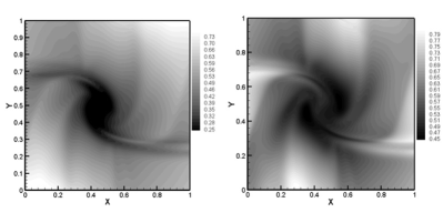
Figure 19: Test 5.7: Distributions of the magnetic energy and pressure.

The problem is solved in the square domain with side dimension $L=1$. The uniform magnetic field ${\bf B}=(2,0,1)$ is imposed. A numerical solution is computed up to time of $t=0.8$ on the mesh of $400\times 400$ with the Courant number of $\beta=0.1$, the parameter $\alpha=0.4$, the adiabatic index $\gamma=1.4$. Gradients of all parameters were equal to zero on the domain boundary. Figs. 18-19 show results of the numerical solution at $t=0.8$. In the center of the square, a rarefied area forms with lower pressure and magnetic energy, the magnetic field lines are strongly curved and diverge. In the middle of the square far from the center on the edges of the vortex area, formation of the compression waves can be seen with increasing of the density, pressure, magnetic energy and a large concentration of the magnetic field lines. Contour lines of the density and magnetic energy describe the structure of the vortex flow with enough precision.

5.8 Orszag-Tang Vortex

In this problem, the formation of the complex structure of shock waves in supersonic turbulence is considered (Arminjon et al., 2005). The problem is solved in square domain with side $L=1$. Initial conditions are given by:

$$\rho=25/(36\pi),p=5/(12\pi),u_{x}=-\sin(2\pi y),u_{y}=\sin(2\pi x),$$

$$u_{z}=0,B_{x}=-B_{0}\sin(2\pi y),B_{y}=B_{0}\sin(4\pi x),B_{z}=0,$$

A solution is computed up to time $t=2$ on the meshes $400\times 400$ and $800\times 800$ with the Courant number of $\beta=0.2$ and the parameter $\alpha=0.3$, the adiabatic index $\gamma=5/3$. Periodic boundary conditions were used. Fig. 20 shows distribution of the pressure contour lines at time $t=0.5$.

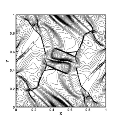
Figure 20: Test 5.8: Distribution of the pressure contour lines in the range of $0.05$ to $0.5$ with step $0.015$ at the moment $t=0.5$.

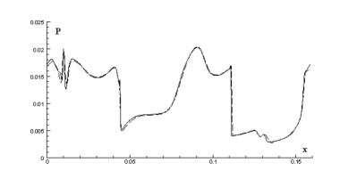
Figure 21: Test 5.8: Pressure along line $y=0.3125$.

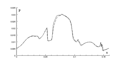
Figure 22: Test 5.8: Pressure along line $y=0.4277$.

Figs. 21-22 show distributions of pressure in the two-dimensional plane sections along the lines $y=0.3125(j=130)$ and $y=0.4277(j=176)$, allowing to estimate a reproducing accuracy of the discontinuities in the solution. Result on mesh with $N=400$ is depicted by dash line and solid line for $N=800$. Fig. 23 shows distribution of the pressure and magnetic energy contour lines for $t=0.5$ on the mesh of $800\times 800$. Comparing to the results, obtained with the high-order PPML method (Ustyugov et al., 2009), we can say that QMHD gives the correct structure of the flow with all discontinuities. On the fine grid the accuracy of QMHD is acceptable.

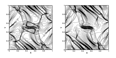
Figure 23: Test 5.8: Distributions pressure and magnetic energy on the mesh $800\times 800$

5.9 Interaction of a shock wave with a cloud

The problem of a cloud destruction by a shock wave in a magnetic field (Tóth, 2000) is considered here. The problem is solved in a square domain with a side $L=1$. In the initial moment of time, two stationary states are defined

$$U_{l}=(3.86859,11.2536,0,0,167.345,$$

$$0,2.1826182,-2.1826182),$$

$$U_{r}=(1,0,0,0,1,0,0.56418958,0.56418958),$$

related to the shock wave, and separated by a plane $x=0.05$.

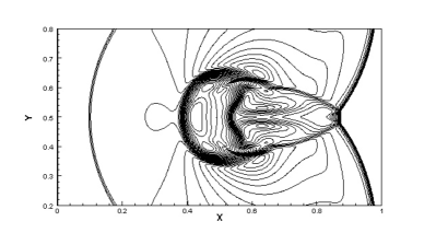
Figure 24: Test 5.9: The contours represent levels of logarithm of the density.

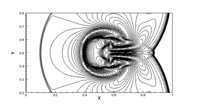
Figure 25: Test 5.9: The same for logarithm of the magnetic energy.

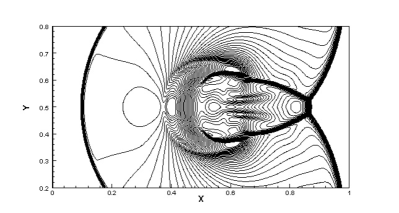
Figure 26: Test 5.9: The same for logarithm of the pressure.

A spherical cloud with density $\rho=10$ and radius $r=0.15$ is set in hydrostatic equilibrium with the environment at the point with coordinates $(0.3,0.5)$. The solution is computed at time moment of $t=0.06$ on the mesh of $400\times 400$ with the Courant number $\beta=0.1$, the parameter $\alpha=0.4$. The adiabatic index $\gamma=5/3$. Gradients of all parameters were equal to zero on the domain boundary. Figs. 24-26 show distributions of contour levels of logarithm of the density, magnetic energy and pressure correspondingly.

6 Conclusions

In this paper, we presented the extension of quasi-gas dynamic approach for a solution of ideal problems of magnetohydrodynamics. We obtained the regularized, or quasi-gas dynamic (QMHD) system of equations for ideal magnetohydrodynamics by applying temporal averaging to all physical parameters, including the magnetic field. The numerical QMHD scheme is multidimensional, where evolution of all physical quantities is carried out in unsplit form by space directions.

It is shown that based on a single approach, the QMHD computational method applied for a compressible magnetohydrodynamics allows modeling a wide range of non-stationary MHD problems. For all studied test cases, computation shows steady converging of numerical solution to its exact solution with shredding of space mesh, providing accurate representation of distribution for all physical quantities on smooth part of a solution and on discontinuities as well. With adjustment of the tuning parameters the quality of the numerical solution may be increased.

The tests of Orszag-Tang vortex, a blast wave propagation through magnetized medium, and interaction of a shock wave with a cloud have been solved recently by QMHD scheme for full 3D case (Popov et al., 2013). The value of tuning parameters $\alpha=0.5$, $Sc=Pr=1$ are suitable for all problems in 1D, 2D and 3D cases.

Simplicity of numerical realization and uniformity of the algorithm provides natural realization on parallel computer systems implying domain-decomposition technique. The second makes QMHD approach promising for numerical solution of complex 3D MHD problems.

The disadvantage of the QMHD method is the first-order approximation, that requires more detailed computational mesh to obtain the quality of a solution in comparison to high-order schemes, such as PPML. On the other hand, the high approximation orders are a little bit formal since they are true only for smooth solutions, whereas in most interesting applications the solutions are discontinuous .

Still QMHD method is robust, relatively cheap by computational cost and requires no additional monotonization procedures, e.g. limiting functions, what is very nice property especially for magnetohydrodynamic simulations.

References

- Almgren et al. (2010) Almgren A. S. et al. CASTRO: a new compressible astrophysical solver. I. Hydrodynamics and self-gravity. Astrophys. J. 2010; 715 1221–1238.
- Arminjon et al. (2005) Arminjon P., Touma R. Central finite volume methods with constrained transport divergence treatment for ideal MHD. J. Comput. Phys. 2005; 204: 737–759.
- Balsara (1998) Balsara D. S. Total variation diminishing scheme for adiabatic and isothermal magnetohydrodynamics. Astrophys. J. Suppl. Series 1998; 116: 133–153.
- Bird (1994) Bird M., Molecular gas dynamics and the direct simulation of gas flows. – Oxford: Clarendon Press, 1994.
- Brio (1988) Brio M., Wu C. C. An upwind differencing scheme for the equations of ideal magnetohydrodynamics. J. Comput. Phys. 1988; 75: 400–422.
- Chetverushkin (2008) Chetverushkin B. N. Kinetic schemes and Quasi-Gas Dynamic System of Equations. CIMNE: Barselona, 2008.
- Chpoun et al. (2005) Chpoun A., Elizarova T. G., Graur I. A., Lengrand J. C. Simulation of the rarefied gas flow around a perpendicular disk. Europ. J. of Mechanics (B/Fluids) 2005; 24: 457–467.
- Dai et al. (1994) Dai W., Woodward P. Extension of the Piecewise Parabolic Method to multidimensional ideal magnetohydrodynamics. J. Comput. Phys. 1994; 115: 485–514.
- Dai et al. (1998) Dai W., Woodward P. A simple finite difference scheme for multidimensional magnetohydrodynamical equations. J. Comput. Phys. 1998; 142: 331–369.
- Ducomet et al. (2013) Ducomet B., Zlotnik A. On a regularization of the magnetic gas dynamics system of equations. Kinetic Theory and Related Models 2013; accepted [http://arxiv.org/abs/1211.3539].
- Elizarova et al. (2001) Elizarova T. G., Graur I. A., Lengrand J.-C. Two-fluid computational model for a binary gas mixture. Europ. J. of Mechanics (B/Fluids) 2001; 3: 351–369.
- Elizarova (2009) Elizarova T. G. Quasi-Gas Dynamic Equations. Springer, 2009.
- Elizarova et al. (2009) Elizarova T. G., Shil’nikov E. V. Capabilities of a Quasi-Gasdynamic Algorithm as Applied to Inviscid Gas Flow Simulation. Comp. Mathem. and Mathem. Phys. 2009; 49: 532–548.
- Elizarova et al. (2011a) Elizarova T. G., Ustyugov S. D. Quasi-gas dynamic algorithm of solution of magnetohydrodynamic equations. One dimensional case. Preprint of Keldysh Institute of Applied Mathematics 2011; 30: 24 pages [in Russian] http://library.keldysh.ru/preprint.asp?id=2011-30
- Elizarova et al. (2011b) Elizarova T. G., Ustyugov S. D. Quasi-gas dynamic algorithm of solution of magnetohydrodynamic equations. Multidimensional case. Preprint of Keldysh Institute of Applied Mathematics 2011; 1: 20 pages [in Russian] http://library.keldysh.ru/preprint.asp?id=2011-1
- Elizarova (2011) Elizarova T. G. Time Averaging as an Approximate Technique for Constructing Quasi-Gasdynamic and Quasi-Hydrodynamic Equations. Comput. Mathem. and Mathem. Phys. 2011; 51: 1973–1982.
- Fryxell B. et al. (2000) Fryxell B. et al. FLASH: An Adaptive mesh hydrodynamics code for modeling astrophysical thermonuclear flashes. Astrophys. J. Suppl. Ser. 2000; 131: 273–334.
- Gardiner et al. (2005) Gardiner T. A., Stone J. M. An unsplit Godunov method for ideal MHD via constrained transport. J. Comput. Phys. 2005; 205: 509–539.
- Graur et al. (2004) Graur I. A., Elizarova T. G., Ramos A., Tejeda G., Fernandez J. M., Montero S. A study of shock waves in expanding flows on the basis of spectroscopic experiments and quasi-gasdynamic equations. J. Fluid Mechanics 2004; 504: 239–270.
- Jiang et al. (1999) Jiang G. S., Wu C. C. A high-order WENO finite difference scheme for the equations of ideal magnetohydrodynamics. J. Comput. Phys. 1999; 150: 561–594.
- Jiang et al. (2012) Jiang R.-L., Fang C., Chen P.-F. A new MHD code with adaptive mesh refinement and parallelization for astrophysics. Comput. Phys. Communicat. 2012; 183: 1617–1633.
- Li (2005) Li S. An HLLC Riemann solver for magneto-hydrodynamics. J. Comput. Phys. 2005; 203: 344–357.
- Mate et al. (2001) Mate B.,Graur I. A., Elizarova T., Chirokov I., Tejeda G., Fernandez J. M., Montero S. Experimental and numerical investigation of an axisymmetric supersonic jet. J. Fluid Mechanics 2001; 426: 177–197.
- Miyoshi et al. (2005) Miyoshi T., Kusano K. A multi-state HLL approximate Riemann solver for ideal magnetohydrodynamics. J. Comput. Phys. 2005; 208: 315–344.
- O’Shea B. et al. (2005) O’Shea B. et al. Introducing Enzo, an AMR cosmology application // adaptive mesh refinement – theory and applications, lecture notes. Comput. Sci. and Engng. Berlin: Springer-Verlag 2005; 41: 341–350. [astroph/0403044].
- Popov et al. (2008) Popov M. V., Ustyugov S. D. Piecewise Parabolic Method on Local Stencil for Ideal Magneto-hydrodynamics. Comput. Mathem. and Mathem. Phys. 2008; 48: 477–499.
- Popov et al. (2013) Popov M. V., Elizarova T. G. Simulation of 3D flows in magneto quasi-gasdynamics. Preprint of Keldysh Institute of Applied Mathematics 2013; 23: 32 pages [in Russian] http://library.keldysh.ru/preprint.asp?id=2013-23
- Tóth et al. (1996) Tóth G., Odstrcil D. Comparison of Some Flux Corrected Transport and Total Variation Diminishing Numerical Schemes for Hydrodynamic and Magnetohydrodynamic Problems. J. Comput. Phys. 1996; 128: 82–100.
- Tóth (2000) Tóth G. The constraint in shock-capturing magnetohydrodynamics codes. J. Comput. Phys. 2000; 161: 605–652.
- Ustyugov et al. (2009) Ustyugov S. D., Popov M. V., Kritsuk A. G., Norman M. L. Piecewise Parabolic Method on a Local Stencil for Magnetized Supersonic Turbulence Simulation. J. Comput. Phys. 2009; 228: 7614–7633.
- Sheretov (2009) Sheretov Yu. V. Dynamic of Continuous Medium in Spatio-Time Averaging. SPC ”Regular and Caotic Dynamics”: Moscow-Izhevsk, 2009.
- Stone et al. (2008) Stone J. M., Gardiner T. A., Teuben P. et al. Athena: a new code for astrophysical MHD. Astrophys. J. Suppl. Ser. 2008; 178: 137–177.
- Sturrock (1994) Sturrock P. A. Plasma Physics: An Introduction to the Theory of Astrophysical, Geophysical, and Laboratory Plasmas. Cambridge University Press, 1994.
- Yu et al. (2001) Yu. H., Liu, Y.-P. A Second-Order Accurate, Component-Wise TVD Scheme for Nonlinear, Hyperbolic Conservation Laws. J. Comput. Phys. 2001; 173: 1–16.