ICRR-Report-653-2013-2

IPMU 13-0104

Domain wall and isocurvature perturbation problems
in axion models

Masahiro Kawasaki^a,b, Tsutomu T. Yanagida^b and Kazuyoshi Yoshino^a

^aInstitute for Cosmic Ray Research, University of Tokyo, Kashiwa, Chiba 277-8582, Japan
^bKavli Institute for the Physics and Mathematics of the Universe(WPI), Todai Institutes for Advanced Study,, University of Tokyo, Kashiwa, Chiba 277-8583, Japan

Axion models have two serious cosmological problems, domain wall and isocurvature perturbation problems. In order to solve these problems we investigate the Linde’s model in which the field value of the Peccei-Quinn (PQ) scalar is large during inflation. In this model the fluctuations of the PQ field grow after inflation through the parametric resonance and stable axionic strings may be produced, which results in the domain wall problem. We study formation of axionic strings using lattice simulations. It is found that in chaotic inflation the axion model is free from both the domain wall and the isocurvature perturbation problems if the initial misalignment angle $\theta_{a}$ is smaller than $O(10^{-2})$. Furthermore, axions can also account for the dark matter for the breaking scale $v\simeq 10^{12-16}\,\mathrm{GeV}$ and the Hubble parameter during inflation $H_{\mathrm{inf}}\lesssim 10^{11-12}\,\mathrm{GeV}$ in general inflation models.

1 Introduction

Axion [1] is a scalar particle predicted in Peccei-Quinn (PQ) mechanism [2] which is a natural solution to the strong CP problem in QCD. In the PQ mechanism there exits a compelex scalar field with global $U(1)_{\mathrm{PQ}}$ symmetry. The $U(1)_{\mathrm{PQ}}$ symmetry is spontaneously broken at some scale $v$ and axion is a Nambu-Goldstone boson associated with it. The axion is also attractive in cosmology because the coherent oscillation of the axion field behaves like the nonrelativistic fluid and can be a good candidate for the dark matter of the universe [3].

In the cosmological scenario, however, the axion models cause the domain wall problem [4]. When the cosmic temperature falls to the symmetry breaking scale $v$, $U(1)_{\mathrm{PQ}}$ symmetry is spontaneously broken, which leads to formation of one-dimensional topological defects called axionic strings. Furthermore, when the cosmic temperature cools down as low as the QCD scale, the axion potential is lifted up through the QCD instanton effect and the axion acquires its mass. Since the axion potential has $N_{\rm DW}$ ($N_{\rm DW}$ is called domain wall number) desecrate minima and the axion field settles down to one of the minima, domain walls are formed so that $N_{\rm DW}$ domain walls attach each string. $N_{\rm DW}$ is determined by QCD anomaly and it depends on details of axion models. For example, $N_{\mathrm{DW}}$ is the number of heavy quarks which have $U(1)_{\mathrm{PQ}}$ charge in the KSVZ model [5], while it is double of the number of generations, i.e. $N_{\rm DW}=6$, in the DFSZ model [6]. It is known that stable domain walls are disastrous in cosmology because they dominate the universe soon after their formation and overclose the universe, which contradicts the present observations.

There are a few solutions to the domain wall problem. One is the $N_{\mathrm{DW}}=1$ model which can be realized in the KSVZ model. The domain walls with $N_{\mathrm{DW}}=1$ are disk-like objects whose boundaries are strings and they collapse by their tension [7]. Thus, string-wall networks with $N_{\mathrm{DW}}=1$ are unstable. In this case, domain walls decay into axion particles soon after their formation. In Ref. [8] the spectrum of axions radiated from strings and domain walls is calculated numerically and it was found that the axion decay constant $F_{a}$, which is related with the PQ breaking scale as $v=N_{\mathrm{DW}}F_{a}$, should satisfy $F_{a}\lesssim(2.0-3.8)\times 10^{10}\,\mathrm{GeV}$ in order that the axion abundance does not exceed the dark matter abundance. Another solution for $N_{\mathrm{DW}}\geq 2$ is to postulate the bias parameter which breaks the PQ symmetry explicitly [4]. Due to the bias, the degeneracy of the potential minimum is resolved and domain walls become unstable. However, this bias also shifts the minimum of the axion potential and hence violates CP. In Ref. [9] it was found that the phase of the bias parameter needs to be fine-tuned in order to satisfy the constraint from CP violation as well as cosmological and astrophysical constraints.

The above arguments apply to the case where the PQ symmetry breaking occurs after inflation. Assuming that the PQ symmetry is spontaneously broken before or during inflation, the domain wall problem is expected to be solved for the general domain number $N_{\mathrm{DW}}$ because the exponential cosmic expansion during inflation makes the value of the axion field homogeneous in the whole observable universe. However, the axion field obtains fluctuation $\delta a=H_{\mathrm{inf}}/2\pi$ with $H_{\mathrm{inf}}$ being the Hubble parameter during inflation, which leads to large isocurvature density perturbations [10, 11, 12, 13, 14, 15]. The isocurvature density perturbations are stringently constrained by cosmic microwave background (CMB) observations [16, 17]. Therefore, when the PQ symmetry breaking takes place during or before inflation, we have another cosmological difficulty, i.e., isocurvature perturbation problem. In particular, this problem is serious for the chaotic inflation model [18] because of its large Hubble parameter during inflation and the axion model may be inconsistent with chaotic inflation.

In Ref. [19], Linde proposed that the large expectation value in the radial direction of the PQ field during inflation can suppress the isocurvature perturbations and it can avoid the domain wall problem simultaneously. After inflation, though, the large fluctuations of the PQ field are generated by the parametric resonance [20, 21, 22] and they can lead to nonthermal restoration of the $U(1)_{\mathrm{PQ}}$ symmetry [23, 24, 25, 26]. Then, stable axionic strings are formed at the subsequent $U(1)_{\mathrm{PQ}}$ symmetry breaking and eventually the domain wall problem comes again after the QCD phase transition  [27, 28]. The formation of the stable strings with the nonthermal symmetry restoration was calculated using lattice simulations in the radiation dominated background after chaotic inflation with quartic potential in Ref. [29]. It was found that the $U(1)_{\mathrm{PQ}}$ symmetry breaking scale must satisfy $v\gtrsim 3\times 10^{16}\,\mathrm{GeV}$ in order that the stable axionic strings which lead to the domain wall problem are not formed.

In this paper, we reexamine the formation of the axionic strings in Linde’s model using lattice simulation. We assume that the universe is matter dominated after inflation in contrast to Ref. [29], which is natural when the inflaton oscillates along the quadratic potential. We find that the constraint on the PQ breaking scale is much relaxed as $v\gtrsim 10^{-4}\left|\Phi\right|_{i}$, where $\left|\Phi\right|_{i}$ represents the initial value of the PQ field. Together with observational constrains, it is found that chaotic inflation is consistent with the axion model if the initial misalignment angle $\theta_{a}$ is less than $O(10^{-2})$. Furthermore, we find that axion can be dark matter without the isocurvature perturbation problem nor the domain wall problem for $v\simeq 10^{12-16}\,\mathrm{GeV}$ and $H_{\mathrm{inf}}\lesssim 10^{11-12}\,\mathrm{GeV}$ in general inflation models.

This paper is organized as follows. Section 2 introduces our model and studies the analytical prediction for the constraint of $U(1)_{\mathrm{PQ}}$ breaking scale. In Section 3, the numerical simulation for the nonlinear dynamics after inflation is carried out. Section 4 describes the observational constraints on the model parameters. We summaries our conclusion in Section 5.

2 Dynamics of the Fields

Let us consider an inflaton field $\chi$ and a complex PQ field $\Phi$ with the potential

$$V=\frac{M^{2}}{2}\chi^{2}+\frac{\lambda}{2}\left(\left|\Phi\right|^{2}-v^{2}\right)^{2},$$ (1)

where $M$ is the mass of the inflaton, $\lambda$ is a self-coupling constant of the PQ field and $v$ is the breaking scale of $U(1)_{\mathrm{PQ}}$ symmetry. Here, for concreteness we consider the chaotic inflation model and the inflaton has a value larger than Planck scale during inflation. We assume that the value in the radial direction of the PQ field during inflation is large enough to satisfy the observational constraint on isocurvature perturbations. When the PQ field satisfies the slow-roll condition, it follows the attractor solution given by [30]

$$\left|\Phi\right|=\frac{M}{\sqrt{2\lambda}}\left(\ln\frac{\chi_{0}}{\chi}\right)^{-1/2},$$ (2)

where $\chi_{0}$ is the inflaton value when the inflaton escapes from the stochastic region, given by

$$\chi_{0}\sim 3\times 10^{3}M_{\mathrm{p}}\left(\frac{10^{13}\,\mathrm{GeV}}{M}\right)^{1/2}.$$ (3)

In the chaotic inflation model, the field value of the inflaton corresponding to e-folding number $N=60$ is $\chi_{N=60}\simeq 15M_{\mathrm{p}}$ and the inflation ends at $\chi_{\mathrm{end}}=\sqrt{2}M_{\mathrm{p}}$. Therefore, from Eqs. (2) and (3) we obtain $\left|\Phi\right|_{N=60}\simeq 1.2\left|\Phi\right|_{\mathrm{end}}$. Namely, the PQ field hardly move during inflation.

After inflation the universe is dominated by the oscillation of the inflaton. Since the effective mass of the PQ field in the radial direction is $m_{\mathrm{eff}}\simeq\sqrt{3\lambda}\left|\Phi\right|\simeq 0.8H$ at the end of inflation, the PQ field starts to oscillate soon after inflation. When the amplitude of the PQ field is much larger than $v$, the potentail of the PQ field is approximately quartic and the amplitude of the PQ field oscillation decreases as $a^{-1}$. Thus, the scale factor $a_{c}$ when the PQ field settles down to the minimum of its potential is estimated as

$$a_{c}\simeq\frac{\left|\Phi\right|_{i}}{v}a_{i},$$ (4)

where the subscript $``\,i\,"$ represents the initial time at the beginning of oscillation. Hereafter we adopt the normalization as $a_{i}=1$.

Until the homogeneous mode of the PQ field settles down to the potential minimum, the fluctuations of the PQ field grow exponentially through the parametric resonance. If the amplitude of the fluctuations $\delta\Phi$ become larger than $v$, the effective potential is lifted up and the PQ symmetry is restored nonthermally. After that, the fluctuations decrease by the cosmic expansion, $U(1)_{\mathrm{PQ}}$ symmetry is spontaneously broken again and stable cosmic strings which lead to the domain wall formation may eventually be formed.

We perform lattice simulations and examine whether stable cosmic strings are formed or not. Before showing the results of the numerical simulations, let us estimate the order of the PQ scale $v$ for strings not to be formed. We define two real scalar fields $X=\mathrm{Re}\,\Phi$ and $Y=\mathrm{Im}\,\Phi$, and these two fields can be decomposed into their homogeneous parts and fluctuations as $X=\bar{X}+\delta X$ and $Y=\bar{Y}+\delta Y$ with the initial conditioins $\bar{X}_{i}=\left|\Phi\right|_{i},\bar{Y}_{i}=0$. When the amplitude of $\bar{X}$ is much larger than $v$, the time evolution of $\bar{X}$ is approximately given by [31]

$$\bar{X}(\tau)\simeq\frac{\left|\Phi\right|_{i}}{a(\tau)}\cos\left(c\sqrt{\lambda}\left|\Phi\right|_{i}\left(\tau-\tau_{\mathrm{i}}\right)\right),$$ (5)

where $\tau=\int dt/a$ is the conformal time and $c\simeq 0.8472$ is a constant. The linearized equations of motion of the fluctuations in Fourier space are

$$\ddot{\delta X}_{k}+3H\dot{\delta X}_{k}-\frac{k^{2}}{a^{2}}\delta X_{k}+\lambda\left(3\bar{X}^{2}-v^{2}\right)\delta X_{k} = 0,$$ (6)

$$\ddot{\delta Y}_{k}+3H\dot{\delta Y}_{k}-\frac{k^{2}}{a^{2}}\delta Y_{k}+\lambda\left(\bar{X}^{2}-v^{2}\right)\delta Y_{k} = 0.$$ (7)

Rescaling as $z=c\sqrt{\lambda}\left|\Phi\right|_{i}\left(\tau-\tau_{i}\right)$, $\delta x_{k}=a\delta X_{k}$, $\delta y_{k}=a\delta Y_{k}$, Eqs. (6) and (7) become Mathieu equation:

$$\frac{d^{2}\delta x_{k}}{dz^{2}}+\left[A_{x}+2q_{x}\cos 2z\right]\delta x_{k} \simeq 0,$$ (8)

$$\frac{d^{2}\delta y_{k}}{dz^{2}}+\left[A_{y}+2q_{y}\cos 2z\right]\delta y_{k} \simeq 0,$$ (9)

where

$$A_{x}=\frac{k^{2}-a^{2}\lambda v^{2}}{c^{2}\lambda\left|\Phi\right|_{i}^{2}}+2q_{x},\ \ A_{y}=\frac{k^{2}-a^{2}\lambda v^{2}}{c^{2}\lambda\left|\Phi\right|_{i}^{2}}+2q_{y},\ \ q_{x}=\frac{3}{4c^{2}},\ \ q_{y}=\frac{1}{4c^{2}}.$$

Here we have neglected the term which contains the decreasing factor $\frac{a^{\prime\prime}}{a}=\frac{2}{\tau^{2}}$ for simplicity. From Eq. (4) and $q_{x}\simeq 1.04,q_{y}\simeq 0.35$, $A_{x}$ is larger than unity for any momentum, on the other hand $A_{y}$ can be unity for an appropriate momentum. Therefore the parametric resonance occurs in the first instability band for $\delta y_{k}$, but it occurs in the second instability band for $\delta x_{k}$. Since the resonance of $\delta y_{k}$ is stronger than that of $\delta x_{k}$, the growth of the fluctuations of the imaginary part of the PQ field is faster than that of the real part. This is also understood from the fact that there is no potential in the imaginary direction. Neglecting the fluctuations of the real part $\delta X$ for the above reason, the amplitude of the field fluctuations is estimated as

$$\braket{\left missing}{\delta\Phi}{{}^{2}} \simeq \braket{\delta Y^{2}}$$ (10)

$$= \frac{1}{a^{2}}\int\frac{dk}{k}\frac{k^{3}}{2\pi^{2}}\left|\delta y_{k}\right|^{2}.$$

Assuming that the initial condition for the fluctuations is the flat spectrum $\frac{k^{3}}{2\pi^{2}}\left(\frac{H_{\mathrm{inf}}}{2\pi}\right)^{2}$ which is generated during inflation, and that the first instability band dominates the momentum integration, we have

$$\braket{\left missing}{\delta\Phi}{{}^{2}} \simeq \frac{1}{a^{2}}\left(\frac{H_{\mathrm{inf}}}{2\pi}\right)^{2}\frac{\Delta k_{*}}{k_{*}}e^{2\mu_{k_{*}}z}$$ (11)

$$= \frac{1}{a^{2}}\left(\frac{H_{\mathrm{inf}}}{2\pi}\right)^{2}\frac{1}{4c\sqrt{c^{2}-\frac{1}{2}}}e^{\frac{\sqrt{\lambda}\left|\Phi\right|_{\mathrm{i}}}{4c}\left(\tau-\tau_{i}\right)},$$

where the typical momentum and the width in the first instability band are $k_{*}\simeq\sqrt{\lambda}\left|\Phi\right|_{i}\sqrt{c^{2}-\frac{1}{2}}$ and $\Delta k_{*}\simeq\frac{\sqrt{\lambda}\left|\Phi\right|_{i}}{4c}$, the growth rate of $\delta y_{k}$ in the first instability band is $\mu_{k_{*}}=1/(8c^{2})$ [22]. Moreover, the initial conformal time is $\tau_{i}=\frac{2}{H_{i}}\simeq\frac{2}{\sqrt{3\lambda}\left|\Phi\right|_{i}}$ and the conformal time when the homogeneous mode settles down into the minimum of its potential is $\tau_{c}=\sqrt{\Phi_{i}/v}\,\tau_{i}$ from Eq. (4) since $a\propto\tau^{2}$ and $aH\tau=2$ in the matter dominated universe. From Eq. (11), the condition for strings not to be formed $\braket{\left missing}{\delta\Phi}{{}^{2}}(\tau_{c})\lesssim v^{2}$ is given by

$$v\gtrsim\left|\Phi\right|_{i}\left[1+2\sqrt{3}c\ln\left(16\pi^{2}c\sqrt{c^{2}-\frac{1}{2}}\left(\frac{\left|\Phi\right|_{i}}{H_{\mathrm{inf}}}\right)^{2}\right)\right]^{-2}.$$ (12)

This expression is independent of the self-coupling constant $\lambda$, because the duration of resonance is dependent on only the ratio $\left|\Phi\right|_{i}/v$ from Eq. (4) and the strength of resonance $\sqrt{\lambda}\left|\Phi\right|/m_{\mathrm{eff}}$ is constant. Since the Hubble parameter during the chaotic inflation is $H_{\mathrm{inf}}\simeq 10^{13}\,\mathrm{GeV}$, the above condition is $v\gtrsim 3\times 10^{14}\,\mathrm{GeV}$ for $\left|\Phi\right|_{i}=M_{\mathrm{p}}$, $v\gtrsim 5\times 10^{13}\,\mathrm{GeV}$ for $\left|\Phi\right|_{i}=0.1M_{\mathrm{p}}$ and $v\gtrsim 7\times 10^{12}\,\mathrm{GeV}$ for $\left|\Phi\right|_{i}=0.01M_{\mathrm{p}}$. The results of the numerical simulations in the next section show that Eq. (12) slightly overestimates the condition because the back reaction is not taken into account.

The condition (12) and the result obtained in the next section is much weaker than that given in [29] where the universe is radiation dominated after inflation. Since the scale factor $a$ is proportional to $t^{1/2}$ in the radiation dominated universe, the PQ field oscillates $\sim(|\Phi|_{i}/v)$ times until it settles down to the potential minimum, which should be compared with $\sim(|\Phi|_{i}/v)^{1/2}$ in the case of the matter dominated universe. Thus, the parametric resonance is more significant for the case considered in [29] and the more strong condition is obtained.

3 Numerical Simulations

In order to study the precise evolution of the PQ field after inflation, we have performed the lattice simulation in two dimensions. From Eq. (1) the equation of motion of the PQ field is as follows:

$$\ddot{\Phi}+3H\dot{\Phi}-\frac{\nabla^{2}}{a^{2}}\Phi+\lambda\left(\left|\Phi\right|^{2}-v^{2}\right)\Phi=0.$$ (13)

Let us rescale the variables as

$$d\bar{\tau}=\sqrt{\lambda}\left|\Phi\right|_{i}\frac{dt}{a},\ \ d\bar{x}=\sqrt{\lambda}\left|\Phi\right|_{i}dx,\ \ \varphi=a\frac{\Phi}{\left|\Phi\right|_{i}}.$$ (14)

Then, the initial rescaled conformal time is $\bar{\tau}_{i}=2/\sqrt{3}$ and Eq. (13) is written as

$$\varphi^{\prime\prime}-\frac{2}{\bar{\tau}^{2}}\varphi-\nabla^{2}_{\bar{x}}\varphi+\left[\left|\varphi\right|^{2}-a^{2}\left(\frac{v}{\left|\Phi\right|_{i}}\right)^{2}\right]\varphi=0,$$ (15)

where the prime represents the derivative with respect to $\bar{\tau}$ and we have used the time dependence of the scale factor $a\propto\tau^{2}$ in the matter dominated universe. We solve numerically Eq. (15) on a $1024^{2}$ lattice with the 4th-order symplectic integrator [32, 33]. Since our interest is whether cosmic strings are formed or not, we choose box size which is larger than horizon size and lattice size which is smaller than string width at any time of the simulations for each set of parameters. Furthermore, we choose total number of time steps so that the parametric resonance ends before the final time of every simulation. Table 1 shows some examples of simulation parameters. The initial condition of the fluctuations of the PQ field $\delta\Phi/\Phi_{i}$ is taken as random numbers whose amplitude is in the range between $0$ and $H_{\mathrm{inf}}/(2\pi\left|\Phi\right|_{i})$ because variance of the PQ field fluctuations during inflation is given by $H^{2}_{\mathrm{inf}}/(2\pi)^{2}$. The Hubble parameter during inflation is fixed to $H_{\mathrm{inf}}=10^{13}\,\mathrm{GeV}$ as is required for the chaotic inflation model. In order to check the accuracy of the code, we calculate the total energy density of this system without cosmic expansion and confirm that the energy is conserved with error less than $0.1\%$.

Table 1: Some examples of rescaled comoving box size, rescaled conformal time and resolution of lattice at the end of simulations for some $v$ and $\left|\Phi\right|_{i}$. $\delta_{\mathrm{st}}(=1/\sqrt{\lambda}v)$ represents the width of a string.

$v\,(\mathrm{GeV})$	$\left|\Phi\right|_{i}$	$\bar{L}$	$\bar{\tau}_{f}-\bar{\tau}_{i}$	$\left.{\delta_{\mathrm{st}}\big{/}dx}\right|_{f}$
$7\times 10^{13}$	$M_{\mathrm{p}}$
$7\times 10^{12}$	$0.1M_{\mathrm{p}}$	$350$	$320$	$1.3$
$7\times 10^{11}$	$0.01M_{\mathrm{p}}$
$2\times 10^{14}$	$M_{\mathrm{p}}$
$2\times 10^{13}$	$0.1M_{\mathrm{p}}$	$250$	$200$	$1.6$
$2\times 10^{12}$	$0.01M_{\mathrm{p}}$
$7\times 10^{14}$	$M_{\mathrm{p}}$
$7\times 10^{13}$	$0.1M_{\mathrm{p}}$	$200$	$140$	$1.2$
$7\times 10^{12}$	$0.01M_{\mathrm{p}}$

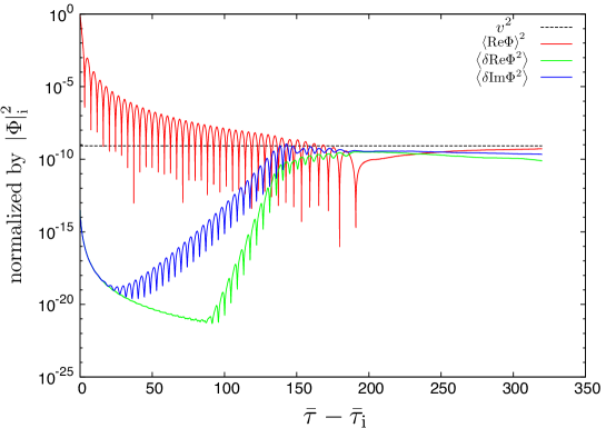
Figure 1: Time evolution of the square of the homogeneous real part of PQ field (red line) and the variances of the real part (green line) and the imaginary part (blue line) for $\left|\Phi\right|_{\mathrm{i}}=M_{\mathrm{p}},v=7\times 10^{13}\,\mathrm{GeV}$. The dashed black line denotes the square of PQ breaking scale. The vertical axis is normalized by the square of the initial amplitude of the homogeneous part $\left|\Phi\right|^{2}_{i}$.

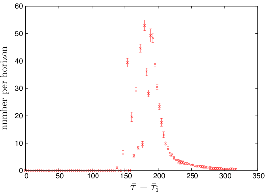
Figure 2: Average number of strings per horizon as the function of conformal time for $\left|\Phi\right|_{i}=M_{\mathrm{p}}$ and $v=7\times 10^{13}~{}\mathrm{GeV}$. We perform the simulation for $10$ realizations.

Varying the breaking scale $v$ of $U(1)_{\mathrm{PQ}}$, we perform the simulations for three initial values; $\left|\Phi\right|_{i}=M_{\mathrm{p}}$, $0.1M_{\mathrm{p}}$ and $0.01M_{\mathrm{p}}$. Fig. 1 shows a example of the evolution of the homogenous part and the variance of the fluctuation of the PQ field for $\left|\Phi\right|_{i}=M_{\mathrm{p}}$ and $v=7\times 10^{13}~{}\mathrm{GeV}$. We define the real part as the direction of the initial value $\Phi_{i}$. As mentioned before, the fluctuations of the imaginary part grows faster than those of the real part because the imaginary part does not have the potential. In Fig. 1, it is found that the amplitude of the fluctuations becomes larger than the breaking scale and the homogeneous part oscillates around the origin with amplitude smaller than the beraking scale $v$. Therefore, the $U(1)_{\mathrm{PQ}}$ symmetry is restored nonthermally and cosmic strings are formed. The number of strings per horizon for these model parameters is shown in Fig. 2. Here, we identify the cosmic strings with the method in [34]. We can find that the exponential growth of the fluctuations is followed by the turbulent stage when many strings are formed, and that the number of strings per horizon remains $O(1)$ after the homogeneous part settles down.

When we search the model parameters for which strings are not formed, there is one subtle problem. In some simulations, strings are temporally formed and disappear soon after the homogeneous part settles, which does not lead to formation of the domain walls. Thus, in this paper, adopting the criterion in [29] we judge stable strings are formed if strings per horizon remains almost constant. From this criterion, we find that the condition for the stable strings not to be formed is $v\gtrsim 2\times 10^{14}~{}\mathrm{GeV}$ for $\left|\Phi\right|_{i}=M_{\mathrm{p}}$, $v\gtrsim 2\times 10^{13}~{}\mathrm{GeV}$ for $\left|\Phi\right|_{i}=0.1M_{\mathrm{p}}$ and $v\gtrsim 2\times 10^{12}~{}\mathrm{GeV}$ for $\left|\Phi\right|_{\mathrm{i}}=0.01M_{\mathrm{p}}$. Performing some simulations with larger grid points $(2048^{2})$ in order to check these results, we confirmed that they are not changed. Therefore, we can derive the following constraint on the breaking scale:

$$v\gtrsim 1\times 10^{-4}\left|\Phi\right|_{i}.$$ (16)

Namely, the growth of the fluctuations of the PQ field depends on only the duration of the homogeneous oscillation determined by the ratio $\left|\Phi\right|_{i}/v$, which is consistent with the analytic estimation (12).

4 Observational Constraints

In this section, we consider the observational constraints on the present axion model. The first constraint comes from the cosmic density of axions. Since the coherent oscillation of the axion field after the QCD phase transition behaves like the nonrelativistic fluid and gives a significant contribution to the dark matter density. Thus, the axion density should satisfy $\Omega_{a}h^{2}\leq\Omega_{\mathrm{CDM}}h^{2}=0.12$ [35].

When axionic strings and domain walls are not formed after inflation, the axion abundance in the present universe is given by [36, 37, 38]

$$\Omega_{a}h^{2}\simeq 0.18\left(\theta^{2}_{a}+\braket{\delta\theta^{2}_{a}}\right)\left(\frac{F_{a}}{10^{12}\,\mathrm{GeV}}\right)^{1.19},$$ (17)

where $F_{a}$ is the axion decay constant, $\theta_{a}$ is the background initial misalignment angle defined by the axion field value at the beginning of coherent oscillation $a_{1}=F_{a}\theta_{a}$ and $\braket{\delta\theta^{2}_{a}}$ is the spatial dispersion of fluctuations generated during inflation. In our model, the radial direction of the PQ field has a large expectation value during inflation. Thus, the fluctuations of misalignment angle can be suppressed as

$$\braket{\delta\theta^{2}_{a}}\simeq\frac{N_{\mathrm{DW}}^{2}}{\left|\braket{\Phi}\right|^{2}}\left(\frac{H_{\mathrm{inf}}}{2\pi}\right)^{2},$$ (18)

where we use the relation between the misalignment angle $\theta_{a}$ and the phase of the PQ field $\theta$, $\theta_{a}=N_{\mathrm{DW}}\theta$.

If axionic strings are formed after inflation, the above expressions are not valid since the misalignment angle has large inhomogeneity in space. Thus, we need to replace $\theta^{2}_{a}+\braket{\delta\theta^{2}_{a}}$ with averaged value $2\times(\pi^{2}/3)$, where we take the anharmonic effect into account [36]. In case of $N_{\mathrm{DW}}\geq 2$, the string-wall system is stable and it leads to the domain wall problem. On the other hand, the domain wall problem can be avoided for $N_{\mathrm{DW}}=1$ since the string-wall system decays soon after formation. In this cace, strings and domain walls decay into axion particles which contribute to the cosmic axion density. In fact, this additional contribution dominates over that from the coherent oscillation and the abundance in the present universe is estimated as [8]

$$\Omega_{a}h^{2}\simeq 8.8\left(\frac{F_{a}}{10^{12}\,\mathrm{GeV}}\right)^{1.19}.$$ (19)

The second constraint is imposed from CMB observations of the CDM isocurvature perterbations. The fluctuations of the axion field during inflation produce the CDM isocurvature perturbations whose power spectrum is given by [39, 40]

$$\mathcal{P}_{\mathcal{S}_{\mathrm{CDM}}}(k)\simeq 4\left(\frac{\Omega_{a}}{\Omega_{\mathrm{CDM}}}\right)^{2}\frac{\mathcal{P}_{\delta\theta_{a}}(k)}{\theta^{2}_{a}+\braket{\delta\theta^{2}_{a}}},$$ (20)

where $\mathcal{P}_{\delta\theta_{a}}(k)$ is the power spectrum of $\delta\theta_{a}$. $\mathcal{P}_{\mathcal{S}_{\mathrm{CDM}}}$ is constrained from the last CMB observation as [17]

$$\beta_{\mathrm{iso}}\equiv\frac{\mathcal{P}_{\mathcal{S}_{\mathrm{CDM}}}(k_{0})}{\mathcal{P}_{\zeta}(k_{0})+\mathcal{P}_{\mathcal{S}_{\mathrm{CDM}}}(k_{0})}<0.036~{}~{}~{}~{}~{}\mathrm{at}~{}~{}95\%~{}\mathrm{CL},$$ (21)

where $\mathcal{P}_{\zeta}(k_{0})$ is the power spectrum of the curvature perturbations and $k_{0}=0.002\,\mathrm{Mpc}^{-1}$. This leads to the constraint on the model parameters via Eq. (20). If strings and domain walls are formed after inflation, perturbations of the misalignment angle generated during inflation disappear due to the restoration of PQ symmetry. Therefore, there is no constraint from the observation of CDM isocurvature perturbations.

4.1 Chaotic inflation model

Now we apply the observational constraints to our model and examine the allowed parameter region. First we assume the chaotic inflation model with the quadratic potential and take the Hubble parameter during inflation to be the large value $H_{\mathrm{inf}}\simeq 10^{13}~{}\mathrm{GeV}$. The cosmological effect of domain walls is quite different between $N_{\mathrm{DW}}=1$ and $N_{\mathrm{DW}}\geq 2$, so we discuss two cases separately.

4.1.1 $N_{\mathrm{DW}}\geq 2$

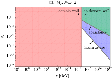
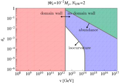
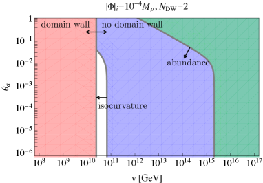
Figure 3: Constraints on $v~{}(=N_{\mathrm{DW}}F_{a})$ and $\theta_{a}$ for $N_{\mathrm{DW}}=2$ and various values of initial amplitude $\left|\Phi\right|_{i}$ in the chaotic inflation model, i.e. $H_{\mathrm{inf}}=10^{13}\,\mathrm{GeV}$. The red region is excluded in order to avoid the domain wall problem from our numerical simulation. The blue region and the green region are excluded by the observation of isocurvature perturbations and dark matter abundance, respectively.

In case of $N_{\mathrm{DW}}\geq 2$, strings and domain walls are stable once they are formed. Therefore, from our numerical simulations the $U(1)_{\mathrm{PQ}}$ breaking scale must satisfy $v\gtrsim 1\times 10^{-4}\left|\Phi\right|_{i}$ in order to avoid the domain wall problem. Fig. 3 shows the result of our simulation and the observational constraints for $N_{\mathrm{DW}}=2$ and three initial conditions $\left|\Phi\right|_{i}=M_{\mathrm{p}}$, $10^{-2}M_{\mathrm{p}}$ and $10^{-4}M_{\mathrm{p}}$. Here, we take the expectation value of the PQ field during inflation to be $\left|\braket{\Phi}\right|=\left|\Phi\right|_{i}$ since the PQ field hardly move during inflation and it starts to oscillate soon after the end of inflation as described in Section 2. It is found that the axion can not be a main component of the dark matter because the constraint from the isocurvature perturbations is much stronger than that from the axion density in the chaotic inflation model. Moreover, the initial misalignment angle must be smaller than $O(10^{-2})$ so that the observational constraints are satisfied. Here it should be noticed that the axion model with $N_{\mathrm{DW}}\geq 2$ can be excluded by the isocurvature perturbation constraint if the PQ scalar settles at the potential minimum ($|\langle\Phi\rangle|=v$) during inflation. Therefore, the present model succeeds in solving the serious isocuravture perturbation problem in chaotic inflation for $|\Phi|_{i}\gg v$. As is seen from Eqs. (17) and (20), this result is almost unchanged even if $N_{\mathrm{DW}}$ is larger than two. In case of $N_{\mathrm{DW}}=6$, for instance, the upper bounds for $\theta_{a}$ and $v$ become about $1.2$ times larger and about $0.5$ times smaller, respectively.

4.1.2 $N_{\mathrm{DW}}=1$

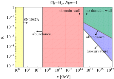
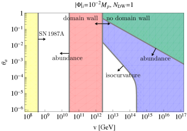
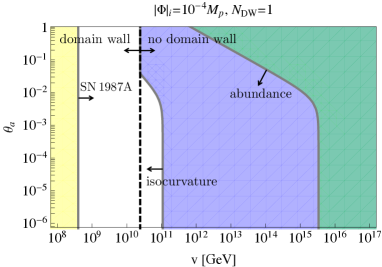
Figure 4: Constraints on $v~{}(=N_{\mathrm{DW}}F_{a})$ and $\theta_{a}$ for $N_{\mathrm{DW}}=1$ and various values of initial amplitude $\left|\Phi\right|_{\mathrm{i}}$ in the chaotic inflation model, i.e. $H_{\mathrm{inf}}=10^{13}\,\mathrm{GeV}$. In the case of $v\gtrsim 10^{-4}\left|\Phi\right|_{i}$, the blue and the green regions are excluded by the observation of the isocurvature perturbations and CDM abundance, respectively. In the case of $v\lesssim 10^{-4}\left|\Phi\right|_{i}$, the red region is the constraint from the axion abundance and the yellow region is excluded by the supernova 1987A.

For $N_{\mathrm{DW}}=1$, the domain wall problem can be solved even if $U(1)_{\mathrm{PQ}}$ symmetry is broken after inflation as mentioned above. Therefore, we consider both regions $v\gtrsim 10^{-4}\left|\Phi\right|_{i}$ and $v\lesssim 10^{-4}\left|\Phi\right|_{i}$. In the former case, the expression for the present axion abundance Eq. (17) and that for the CDM isocurvature perturbation Eq. (20) can be adopted since there is no symmetry restoration after inflation. On the other hand, the axion abundance comes from emission from string-wall system [Eq. (19)] in the latter case. Furthermore, there is another observational constraint coming from the cooling rate of supernova 1987A which imposes the lower limit on axion decay constant as $F_{a}\gtrsim 4\times 10^{8}\,\mathrm{GeV}$ [41]. Fig. 4 shows the parameter regions allowed by the result of the numerical simulations and the observational constraints for $N_{\mathrm{DW}}=1$ and three initial conditions $\left|\Phi\right|_{i}=M_{\mathrm{p}}$, $10^{-2}M_{\mathrm{p}}$ and $10^{-4}M_{\mathrm{p}}$. In the case of $v\gtrsim 10^{-4}\left|\Phi\right|_{i}$, axion can not become a main component of dark matter and the initial misalignment angle must be smaller than $O(10^{-2})$ in the same way as $N_{\mathrm{DW}}\geq 2$. In the case of $v\lesssim 10^{-4}\left|\Phi\right|_{i}$, it is found that axion can become dark matter for $v\simeq 3\times 10^{10}~{}\mathrm{GeV}$ and $\left|\Phi\right|_{i}\gtrsim 10^{-4}M_{\mathrm{p}}$.

4.2 General inflation model

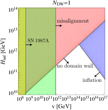
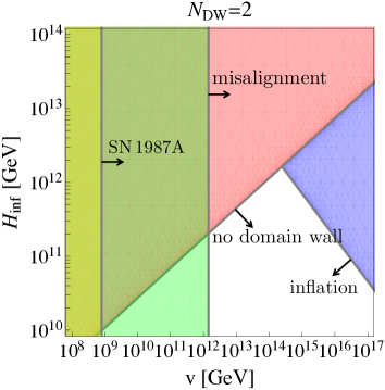
Figure 5: The parameter regions for $v~{}(=N_{\mathrm{DW}}F_{a})$ and $H_{\mathrm{inf}}$ allowed by some conditions and observational constraints in case that axion is the main component of dark matter, $\Omega_{a}h^{2}=\Omega_{\mathrm{CDM}}h^{2}$. The yellow and the green regions represent the observational constraint for the cooling rate of supernova 1987A and the condition for the misalignment angle, $\theta^{2}_{a}+\braket{\delta\theta^{2}_{a}}\lesssim 1$, respectively. The red region is excluded by the constraints for the domain wall problem and CDM isocurvature perturbation. The blue region is the condition for the PQ field not to cause inflation.

So far we have assumed the chaotic inflation model and $H_{\mathrm{inf}}\simeq 10^{13}~{}\mathrm{GeV}$. Now, we consider general models of inflation in which the Hubble parameter $H_{\mathrm{inf}}$ is smaller and inflaton oscillates with the quadratic potential after the end of inflation. The value of the Hubble parameter determines only the initial amplitude of the fluctuations of the PQ field and the exponential growth of its fluctuations is independent of the Hubble parameter from our discussion in Section 2. Therefore, it is expected that the lower limit of the breaking scale $v$ which is necessary to avoid the domain wall problem is scarcely varied when the Hubble parameter changes by a few order. Indeed, performing some simulations for $H_{\mathrm{inf}}=10^{10}~{}\mathrm{GeV}$ and $\left|\Phi\right|_{i}=M_{\mathrm{p}}$, we found that the PQ breaking scale must be larger than $(1-2)\times 10^{14}~{}\mathrm{GeV}$. This is consistent with the above result in the chaotic inflation model in Section 3.

If we impose a condition that axions are the main component of the dark matter $\Omega_{a}h^{2}=\Omega_{\mathrm{CDM}}h^{2}$, the power spectrum of the isocurvature perturbations Eq. (20) is a function of the Hubble parameter $H_{\mathrm{inf}}$, the initial value of the PQ field $\left|\Phi\right|_{i}$, the breaking scale of PQ symmetry $v$ and the domain wall number $N_{\mathrm{DW}}$. Avoiding the domain wall problem constrains the initial value $\left|\Phi\right|_{i}$ to satisfy Eq. (16). In addition, in order for the PQ field not to cause inflation, $\left|\Phi\right|_{i}\lesssim M_{\mathrm{p}}$ is should be satisfied. Since the amplitude of the isocurvature perturbations has a minimum value when $\left|\Phi\right|_{i}$ has the maximum value, it is needed that the power spectrum of the isocurvature perturbations for $\left|\Phi\right|_{i}=10^{4}v$ and $\left|\Phi\right|_{i}=M_{\mathrm{p}}$ satisfies the observational constraint simultaneously as

$$\left.\mathcal{P}_{\mathcal{S}_{\mathrm{CDM}}}(k_{0})\right|_{\left|\Phi\right|_{i}=10^{4}v}<\frac{\beta_{\mathrm{iso}}}{1-\beta_{\mathrm{iso}}}\mathcal{P}_{\zeta}(k_{0}),~{}~{}~{}~{}\left.\mathcal{P}_{\mathcal{S}_{\mathrm{CDM}}}(k_{0})\right|_{\left|\Phi\right|_{i}=M_{\mathrm{p}}}<\frac{\beta_{\mathrm{iso}}}{1-\beta_{\mathrm{iso}}}\mathcal{P}_{\zeta}(k_{0}).$$ (22)

Furthermore, there is a condition that the misalignment angle is less than unity, $\theta^{2}_{a}+\braket{\delta\theta^{2}_{a}}\lesssim 1$, by definition. Fig. 5 shows the constraints Eq. (22) for $\Omega_{a}h^{2}=\Omega_{\mathrm{CDM}}h^{2}$, the lower bound of the breaking scale $v$ from the observation of SN 1987A and the condition for the misalignment angle. From the figure, it is found that axion can be the main component of the dark matter avoiding both domain wall and isocurvautre perturbation problems for $v\simeq 10^{12-16}\,\mathrm{GeV}$ and $H_{\mathrm{inf}}\lesssim 10^{11-12}\,\mathrm{GeV}$ in general inflation models. It should be noticed that the present argument does not apply to the string axion model, i.e. $F_{a}\simeq 10^{16}\,\mathrm{GeV}$ [42, 43], because the dynamics of PQ field is different from that of our model. In practice, for the string axion model the Hubble parameter during inflation should be less than $10^{9}\,\mathrm{GeV}$ in order to avoid the isocurvature problem (e.g. see [40]).

5 Conclusion

We have considered the axion model in which $U(1)_{\mathrm{PQ}}$ symmetry is spontaneously broken during inflation and the value of the PQ field is large enough to suppress the axion isocurvature perturbations. The homogeneous part of the PQ field oscillates along its potential in the matter dominated universe after inflation and their fluctuations grows exponentially due to the parametric resonance through the self-coupling of the PQ field. If the fluctuations is large, the $U(1)_{\mathrm{PQ}}$ symmetry is restored and many stable strings are formed, which results in the domain wall problem. Calculating the formation of stable axionic strings using lattice simulations, we have found that $U(1)_{\mathrm{PQ}}$ breaking scale should satisfy $v\gtrsim 10^{-4}\left|\Phi\right|_{i}$, where $\left|\Phi\right|_{i}$ is the value of PQ field at the beginning of oscillation, for the stable strings not to be formed. This result is much weaker than that in Ref. [29] because it assumed the radiation dominated universe where the parametric resonance is more significant as shown in Section 2. Combining our numerical result with the observational constraints from the matter density of the universe and the CDM isocurvature perturbations, it is found that the axion model is consistent with chaotic inflation if the initial misalignment angle $\theta_{a}$ is less than $O(10^{-2})$. In this case axions can not be the main component of dark matter in the chaotic inflation model with Hubble parameter $H_{\mathrm{inf}}\simeq 10^{13}\,\mathrm{GeV}$. However, when we consider general inflation models axion can account for the dark matter without the domain wall problem nor isocurvature perturbation problem for $v\simeq 10^{12-16}\,\mathrm{GeV}$ and $H_{\mathrm{inf}}\lesssim 10^{12}\,\mathrm{GeV}$. This implies that topological inflation model [44, 45, 46] is marginally allowed since the Hubble parameter during inflation is estimated as $H_{\mathrm{inf}}\simeq 10^{12}\,\mathrm{GeV}$[47].

References

- [1] S. Weinberg, Phys. Rev. Lett. 40, 223 (1978); F. Wilczek, Phys. Rev. Lett. 40, 279 (1978).
- [2] R. D. Peccei and H. R. Quinn, Phys. Rev. D 16, 1791 (1977); Phys. Rev. Lett. 38, 1440 (1977).
- [3] J. Preskill, M. B. Wise and F. Wilczek, Phys. Lett. B 120, 127 (1983); L. F. Abbott and P. Sikivie, Phys. Lett. B 120, 133 (1983); M. Dine and W. Fischler, Phys. Lett. B 120, 137 (1983).
- [4] P. Sikivie, Phys. Rev. Lett. 48, 1156 (1982).
- [5] J. E. Kim, Phys. Rev. Lett. 43, 103 (1979); M. A. Shifman, A. I. Vainshtein and V. I. Zakharov, Nucl. Phys. B 166, 493 (1980).
- [6] M. Dine, W. Fischler and M. Srednicki, Phys. Lett. B 104, 199 (1981); A. R. Zhitnitsky, Sov. J. Nucl. Phys. 31, 260 (1980) [Yad. Fiz. 31, 497 (1980)].
- [7] A. Vilenkin and A. E. Everett, Phys. Rev. Lett. 48, 1867 (1982).
- [8] T. Hiramatsu, M. Kawasaki, K. ’i. Saikawa and T. Sekiguchi, Phys. Rev. D 85, 105020 (2012) [Erratum-ibid. D 86, 089902 (2012)] [arXiv:1202.5851 [hep-ph]].
- [9] T. Hiramatsu, M. Kawasaki, K. ’i. Saikawa and T. Sekiguchi, JCAP 1301, 001 (2013) [arXiv:1207.3166 [hep-ph]].
- [10] M. Axenides, R. H. Brandenberger, M. S. Turner, Phys. Lett. B126, 178 (1983).
- [11] D. Seckel, M. S. Turner, Phys. Rev. D32, 3178 (1985).
- [12] A. D. Linde, Phys. Lett. B158, 375-380 (1985).
- [13] A. D. Linde, D. H. Lyth, Phys. Lett. B246, 353-358 (1990).
- [14] M. S. Turner, F. Wilczek, Phys. Rev. Lett. 66, 5 (1991).
- [15] D. H. Lyth, Phys. Rev. D45, 3394 (1992).
- [16] G. Hinshaw et al. [WMAP Collaboration], arXiv:1212.5226 [astro-ph.CO].
- [17] P. A. R. Ade et al. [Planck Collaboration], arXiv:1303.5082 [astro-ph.CO].
- [18] A. D. Linde, Phys. Lett. B 129, 177 (1983).
- [19] A. D. Linde, Phys. Lett. B 259, 38 (1991).
- [20] L. Kofman, A. D. Linde and A. A. Starobinsky, Phys. Rev. Lett. 76, 1011 (1996) [hep-th/9510119].
- [21] L. Kofman, A. D. Linde and A. A. Starobinsky, Phys. Rev. D 56, 3258 (1997) [hep-ph/9704452].
- [22] Y. Shtanov, J. H. Traschen and R. H. Brandenberger, Phys. Rev. D 51, 5438 (1995) [hep-ph/9407247].
- [23] I. I. Tkachev, Phys. Lett. B 376, 35 (1996) [hep-th/9510146].
- [24] I. Tkachev, S. Khlebnikov, L. Kofman and A. D. Linde, Phys. Lett. B 440, 262 (1998) [hep-ph/9805209].
- [25] S. Kasuya and M. Kawasaki, Phys. Rev. D 56, 7597 (1997) [hep-ph/9703354].
- [26] S. Kasuya and M. Kawasaki, Phys. Rev. D 58, 083516 (1998) [hep-ph/9804429].
- [27] S. Kasuya, M. Kawasaki and T. Yanagida, Phys. Lett. B 409, 94 (1997) [hep-ph/9608405].
- [28] S. Kasuya, M. Kawasaki and T. Yanagida, Phys. Lett. B 415, 117 (1997) [hep-ph/9709202].
- [29] S. Kasuya and M. Kawasaki, Phys. Rev. D 61, 083510 (2000) [hep-ph/9903324].
- [30] K. Harigaya, M. Ibe, M. Kawasaki and T. T. Yanagida, Phys. Rev. D 87, 063514 (2013) [arXiv:1211.3535 [hep-ph]].
- [31] P. B. Greene, L. Kofman, A. D. Linde and A. A. Starobinsky, Phys. Rev. D 56, 6175 (1997) [hep-ph/9705347].
- [32] H. Yoshida, Phys. Lett. A 150, 262 (1990).
- [33] T. Hiramatsu, M. Kawasaki and K. ’i. Saikawa, JCAP 1108, 030 (2011) [arXiv:1012.4558 [astro-ph.CO]].
- [34] T. Hiramatsu, M. Kawasaki, T. Sekiguchi, M. Yamaguchi and J. ’i. Yokoyama, Phys. Rev. D 83, 123531 (2011) [arXiv:1012.5502 [hep-ph]].
- [35] P. A. R. Ade et al. [Planck Collaboration], arXiv:1303.5076 [astro-ph.CO].
- [36] M. S. Turner, Phys. Rev. D 33, 889 (1986).
- [37] K. J. Bae, J. -H. Huh and J. E. Kim, JCAP 0809, 005 (2008) [arXiv:0806.0497 [hep-ph]].
- [38] O. Wantz and E. P. S. Shellard, Phys. Rev. D 82, 123508 (2010) [arXiv:0910.1066 [astro-ph.CO]].
- [39] M. Kawasaki, K. Nakayama, T. Sekiguchi, T. Suyama and F. Takahashi, JCAP 0811, 019 (2008) [arXiv:0808.0009 [astro-ph]].
- [40] C. Hikage, M. Kawasaki, T. Sekiguchi and T. Takahashi, arXiv:1211.1095 [astro-ph.CO].
- [41] G. G. Raffelt, Lect. Notes Phys. 741, 51 (2008) [hep-ph/0611350].
- [42] M. Kawasaki and T. Yanagida, Prog. Theor. Phys. 97, 809 (1997) [hep-ph/9703261].
- [43] P. Svrcek and E. Witten, JHEP 0606, 051 (2006) [hep-th/0605206].
- [44] A. Vilenkin, Phys. Rev. Lett. 72, 3137 (1994) [hep-th/9402085].
- [45] K. I. Izawa, M. Kawasaki and T. Yanagida, Prog. Theor. Phys. 101, 1129 (1999) [hep-ph/9810537].
- [46] M. Kawasaki, N. Sakai, M. Yamaguchi and T. Yanagida, Phys. Rev. D 62, 123507 (2000) [hep-ph/0005073].
- [47] K. Harigaya, M. Kawasaki and T. T. Yanagida, Phys. Lett. B 719, 126 (2013) [arXiv:1211.1770 [hep-ph]].