Variable selection for sparse Dirichlet-multinomial regression with an application to microbiome data analysis

Abstract

With the development of next generation sequencing technology, researchers have now been able to study the microbiome composition using direct sequencing, whose output are bacterial taxa counts for each microbiome sample. One goal of microbiome study is to associate the microbiome composition with environmental covariates. We propose to model the taxa counts using a Dirichlet-multinomial (DM) regression model in order to account for overdispersion of observed counts. The DM regression model can be used for testing the association between taxa composition and covariates using the likelihood ratio test. However, when the number of covariates is large, multiple testing can lead to loss of power. To address the high dimensionality of the problem, we develop a penalized likelihood approach to estimate the regression parameters and to select the variables by imposing a sparse group $\ell_{1}$ penalty to encourage both group-level and within-group sparsity. Such a variable selection procedure can lead to selection of the relevant covariates and their associated bacterial taxa. An efficient block-coordinate descent algorithm is developed to solve the optimization problem. We present extensive simulations to demonstrate that the sparse DM regression can result in better identification of the microbiome-associated covariates than models that ignore overdispersion or only consider the proportions. We demonstrate the power of our method in an analysis of a data set evaluating the effects of nutrient intake on human gut microbiome composition. Our results have clearly shown that the nutrient intake is strongly associated with the human gut microbiome.

T1Supported in part by NIH Grants CA127334, GM097505 and UH2DK083981.

and

1 Introduction

The human body is inhabited by complex microbial communities, called microbiomes. It is estimated that the number of microbial cells associated with the human body is 10 times the total number of human cells. The collective genomes of these microbes constitute an extended human genome that provides us with genetic and metabolic capabilities that we do not inherently possess [Bäckhed et al. (2005)]. With the development of next generation sequencing technology such as the 454 pyrosequencing and Illumina Solexa sequencing, microbiome composition can now be determined by direct DNA sequencing without laborious cultivation. Typically, instead of sequencing all bacterial genomic DNA as in a shotgun metagenomic approach, only the 16S rRNA gene, which is ubiquitous in the bacteria kingdom and has variable regions, is sequenced. Since each bacterial cell is assumed to have the same number of copies of this gene, the basic idea is to isolate from all the bacteria the DNA strands corresponding to some variable region of the gene, to count different versions of the sequences, and then to identify to which bacteria the versions correspond. The types and abundances of different bacteria in a sample can therefore be determined. After preprocessing of the raw sequences, the 16S sequences are either mapped to an existing phylogenetic tree in a taxonomic dependent way [e.g., Matsen, Kodner and Armbrust (2010)] or clustered into operational taxonomic units (OTUs) at a certain similarity level in a taxonomic independent way [e.g., Caporaso et al. (2010), Schloss et al. (2009)]. At 97% similarity level, these OTUs are used to approximate the taxonomic rank species. The OTU based approach is most commonly used in 16S based microbiome studies. Each OTU is characterized by a representative DNA sequence and can be assigned a taxonomic lineage by comparing to a known bacterial 16S rRNA database. Most OTUs are in extremely low abundances, with a large proportion being simply singletons (possibly due to sequencing error). We can further aggregate OTUs from the same genus and perform analysis on the abundances at the genus level, which is more robust to sequencing error and can reduce the number of variables significantly. Either way we finally obtain the taxa counts for each sample.

Recent studies have linked the microbiome with human diseases including obesity and inflammatory bowel disease [Virgin and Todd (2011)]. It is therefore important to understand how genetic or environmental factors shape the human microbiome in order to gain insight into etiology of many microbiome-related diseases and to develop therapeutic measures to modulate the microbiome composition. Benson et al. (2010) demonstrated that genetic variants are associated with the mouse gut microbiome. Wu et al. (2011) showed that dietary nutrients are associated with the human gut microbiome. Both studies have considered a large number of genetic loci or nutrients and aimed to identify the genetic variants or nutrients that are associated with the gut microbiome. When there are numerous possible covariates affecting the microbiome composition, variable selection becomes necessary. Variable selection cannot only increase biological interpretability but also provide researchers with a short list of top candidates for biological validation. The methods we develop in this paper are particularly motivated by an ongoing study at the University of Pennsylvania to link the nutrient intake to the human gut microbiome. In this study, gut microbiome data were collected on 98 normal volunteers. In addition, food frequency questionnaire (FFQ) were filled out by these individuals. The questionnaires were scored and the quantitative measurements of 214 micronutrients were obtained. Details of the study and the data set can be found in Section 6 and in Wu et al. (2011). Our goal is to identify the nutrients that are associated with the gut microbiome and also their associated bacterial taxa.

Most of the microbiome studies used distance-based methods to link the microbiome and environmental covariates, where a distance metric was defined between two microbiome samples and statistical analysis was then performed using the distances. However, the choice of distance metric is sometimes subjective and different distances vary in their power of identifying relevant environmental factors. Another limitation of distance-based methods is its inefficiency for detecting subtle changes since distances summarize the overall relationship. In addition, such distance-based approaches do not provide information on how covariates affect the microbiome compositions and which taxa are affected. Therefore, it is desirable to model the counts directly instead of summarizing the data as distances. One way of testing for covariate effects is by performing a multivariate multiple regression (called redundancy analysis in ecology) after appropriate transformation of the count data such as converting into proportions [Legendre and Legendre (2002)]. A pseudo-$F$ statistic is then calculated and the significance is then evaluated by permutation test. Alternatively, one can define a distance between the samples and then use a PERMANOVA procedure to test for covariate effects [McArdle (2001)]. It is easy to show that when the distance is Euclidean, these two procedures are equivalent.

In this paper, we consider the sparse Dirichlet-multinomial (DM) regression [Mosimann (1962)] to link high-dimensional covariates to bacterial taxa counts from microbiome data. The DM regression model is chosen to model the overdispersed taxa counts. The observed taxa count variance is much larger than that predicted by a multinomial model that assumes fixed underlying taxa proportions, an assumption that is hardly met for real microbiome data. Uncontrollable sources of variation such as individual-to-individual variability, day-to-day variability, sampling location variability or even technical variability such as sample preparation lead to enormous variability in the underlying proportions. In contrast, the DM model assumes that the underlying taxa proportions come from a Dirichlet distribution. We use a log-linear link function to associate the mean taxa proportions with covariates. In this DM modeling framework, the effects of the covariates on taxa proportions can be tested using the likelihood ratio test.

When the number of the covariates is large, we propose a sparse group $\ell_{1}$ penalized likelihood approach for variable selection and parameter estimation. The sparse group $\ell_{1}$ penalty function [Friedman, Hastie and Tibshirani (2010)] consists of a group $\ell_{1}$ penalty and an overall $\ell_{1}$ penalty, which induce both group-level sparsity and within-group sparsity. This is particularly relevant in our setting. For the nutrient-microbiome association example, we have $p$ nutrients and $q$ taxa, so the fully parameterized model has $(p+1)\times q$ coefficients including the intercepts, since each nutrient-taxon association is characterized by one coefficient. The $q$ coefficients for each nutrient constitute a group. If we assume many nutrients have no or ignorable effects on the microbiome composition, the groups of coefficients associated with these irrelevant nutrients should be zero altogether, which is a group-level sparsity that is achieved by imposing a group $\ell_{1}$ penalty. However, the group $\ell_{1}$ penalty does not perform within-group selection, wherein if one group is selected, all the coefficients in that group are nonzeros. In the case of nutrient-microbiome association, we are also interested in knowing which taxa are associated with a selected nutrient. By imposing an overall $\ell_{1}$ penalty, within-group selection becomes possible. Therefore, we impose a sparse group $\ell_{1}$ penalty not only to select these important nutrients but also to recover relevant nutrient-taxon associations.

Section 2 reviews the Dirichlet-multinomial model for count data. Section 3 introduces the Dirichlet-multinomial regression framework for incorporating covariate effects and proposes a likelihood ratio statistic for testing the covariate effect. Section 4 proposes a sparse group $\ell_{1}$ penalized likelihood procedure for variable selection for the DM models followed by a detailed description of a block-coordinate descent algorithm in Section 4.1. Section 5 shows simulation results and Section 6 demonstrates the proposed method on a real human gut microbiome data set to associate the nutrient intake with the human gut microbiome composition.

2 Dirichlet-multinomial model for microbiome composition data

Suppose we have $q$ bacterial taxa and their counts $Y=(Y_{1},Y_{2},\ldots,Y_{q})$ are random variables. Denote ${\mathbf{y}}=(y_{1},y_{2},\ldots,y_{q})$ as the observed counts. The simplest model for count data is the multinomial model and its probability function is given as

$$f_{M}(y_{1},y_{2},\ldots,y_{q};\bolds{\phi})=\pmatrix{y_{+}\cr{\mathbf{y}}}\prod_{j=1}^{q}\phi_{j}^{y_{j}},$$

where $y_{+}=\sum_{j=1}^{q}y_{j}$ and $\bolds{\phi}=(\phi_{1},\phi_{2},\ldots,\phi_{q})$ are underlying species proportions with $\sum_{j=1}^{q}\phi_{j}=1$. Here the total taxa count $y_{+}$ is determined by the sequencing depth and is treated as an ancillary statistic since its distribution does not depend on the parameters in the model. The mean and variance of the multinomial component $Y_{j}$ $(j=1,\ldots,q)$ are

$$\mathrm{E}(Y_{j})=y_{+}\phi_{j},\qquad\operatorname{Var}(Y_{j})=y_{+}\phi_{j}(1-\phi_{j}).$$ (1)

For microbiome composition data, the actual variation is usually larger than what would be predicted by the multinomial model, which assumes fixed underlying proportions. This increased variation is due to the heterogeneity of the microbiome samples and the underlying proportions vary among samples. To account for the extra variation or overdispersion, we assume the underlying proportions $(\phi_{1},\phi_{2},\ldots,\phi_{q})$ are themselves positive random variables $(\Phi_{1},\Phi_{2},\ldots,\Phi_{q})$ subject to the constraint $\sum_{j=1}^{q}\Phi_{j}=1$. One commonly used distribution is the Dirichlet distribution [Mosimann (1962)] with the probability function given by

$$f_{D}(\phi_{1},\phi_{2},\ldots,\phi_{q};\bolds\gamma)=\frac{\Gamma(\gamma_{+})}{\prod_{j=1}^{q}\Gamma(\gamma_{j})}\prod_{j=1}^{q}\phi_{j}^{\gamma_{j}-1},$$

where $\bolds\gamma=(\gamma_{1},\gamma_{2},\ldots,\gamma_{q})$ are positive parameters, $\gamma_{+}=\sum_{j=1}^{q}\gamma_{j}$ and $\Gamma(\cdot)$ is the Gamma function. The mean and variance of the Dirichlet component $\Phi_{j}$ $(j=1,\ldots,q)$ are

$$\mathrm{E}(\Phi_{j})=\frac{\gamma_{j}}{\gamma_{+}},\qquad\operatorname{Var}(\Phi_{j})=\frac{\gamma_{j}(\gamma_{+}-\gamma_{j})}{(1+\gamma_{+})\gamma_{+}^{2}}.$$

The mean is proportional to $\gamma_{j}$ and the variance is controlled by $\gamma_{+}$, which can be regarded as a “precision parameter.” As $\gamma_{+}$ becomes larger, the proportions are more concentrated around the means.

The Dirichlet-multinomial (DM) distribution [Mosimann (1962)] results from a compound multinomial distribution with weights from the Dirichlet distribution (parametrization I):

$$f_{\mathrm{DM}}(y_{1},y_{2},\ldots,y_{q};\bolds\gamma) = \int f_{M}(y_{1},y_{2},\ldots,y_{q};\bolds{\phi})f_{D}(\bolds{\phi};\bolds\gamma)\,d\bolds{\phi}$$

$$= \pmatrix{y_{+}\cr{\mathbf{y}}}\frac{\Gamma(y_{+}+1)\Gamma(\gamma_{+})}{\Gamma(y_{+}+\gamma_{+})}\prod_{j=1}^{q}\frac{\Gamma(y_{j}+\gamma_{j})}{\Gamma(\gamma_{j})\Gamma(y_{j}+1)}.$$

The mean and variance of the DM distribution for each component $Y_{j}$ $(j=1,\ldots,q)$ is given by

$$\mathrm{E}(Y_{j})=y_{+}\mathrm{E}(\Phi_{j}),\qquad\operatorname{Var}(Y_{j})=y_{+}\mathrm{E}(\Phi_{j})\bigl{\{}1-\mathrm{E}(\Phi_{j})\bigr{\}}\biggl{(}\frac{y_{+}+\gamma_{+}}{1+\gamma_{+}}\biggr{)}.$$ (3)

Comparing (3) with (1), we see that the variation of the DM component is increased by a factor of $(y_{+}+\gamma_{+})/(1+\gamma_{+})$, where $\gamma_{+}$ controls the degree of overdispersion with a larger value indicating less overdispersion. Using an alternative parameterization, the probability function can be written as (parameterization II)

$$f_{\mathrm{DM}}^{*}(y_{1},y_{2},\ldots,y_{q};\bolds{\phi},\theta)=\pmatrix{y_{+}\cr{\mathbf{y}}}\frac{\prod_{j=1}^{q}\prod_{k=1}^{y_{j}}\{\phi_{j}(1-\theta)+(k-1)\theta\}}{\prod_{k=1}^{y_{+}}\{1-\theta+(k-1)\theta\}},$$ (4)

where $\phi_{j}=\gamma_{j}/\gamma_{+}$ is the mean and $\theta=1/(1+\gamma_{+})$ is the dispersion parameter. When $\theta=0$, it is easy to verify (4) is reduced to the multinomial distribution.

3 Dirichlet-multinomial regression for incorporating the covariate effects

When there is no covariate effect, the DM model can be used to produce more accurate estimates of taxa proportions of a given microbiome sample than the simple multinomial model, due to its ability to model the overdispersion. Beyond proportion estimation, microbial ecologists are more interested in associating the microbiome composition with some environmental covariates. Suppose we have $n$ microbiome samples and $q$ species. Let ${\mathbf{Y}}=(y_{ij})_{n\times q}$ be the observed count matrix for the $n$ samples. Let ${\mathbf{X}}=(x_{ij})_{n\times p}$ be the design matrix of $p$ covariates for $n$ samples. We assume the parameters $\gamma_{j}$ $(j=1,\ldots,q)$ in the DM model (parametrization I) depend on the covariate via the following log-linear model,

$$\gamma_{j}\bigl{(}{\mathbf{x}}^{i}\bigr{)}=\exp\Biggl{(}\alpha_{j}+\sum_{k=1}^{p}\beta_{jk}x_{ik}\Biggr{)},$$ (5)

where ${\mathbf{x}}^{i}$ is the $i$th row vector of ${\mathbf{X}}$ and $\beta_{jk}$ is the coefficient for the $j$th taxon with respect to $k$th covariate, whose sign and magnitude measure the effect of the $k$th covariate on the $j$th taxon. From (3), we see that $\mathrm{E}(Y_{ij})\propto\exp(\alpha_{j})\prod_{k=1}^{p}\exp(\beta_{jk}x_{ik})$, where $\exp(\alpha_{j})$ can be interpreted as the baseline abundance level for species $j$ and the coefficient $\beta_{jk}$ indicates the magnitude of the $k$th covariate effect on species $j$. Though the log-linear link is assumed mainly for ease of computation, it is biologically consistent, in that microorganisms usually exhibit exponential growth in a favorable environment.

For notational simplicity, we denote $\beta_{j0}$ as $\alpha_{j}$ and augment ${\mathbf{X}}$ with an $n$-vector of $1$’s as its first column. We number the columns from $0$ to $p$. The link function becomes

$$\gamma_{j}\bigl{(}{\mathbf{x}}^{i}\bigr{)}=\exp\Biggl{(}\sum_{k=0}^{p}\beta_{jk}x_{ik}\Biggr{)}.$$ (6)

Let $\bolds{\beta}$ be the $q\times(p+1)$ regression coefficient matrix, $\bolds{\beta}^{j}=(\beta_{j0},\ldots,\beta_{jp})^{T}$ be the vector of coefficients for the $j$th taxon ($j=1,\ldots,q$) and $\bolds{\beta}_{k}=(\beta_{1k},\ldots,\break\beta_{qk})^{T}$ be the vector of coefficients for the $k$th covariate ($k=0,\ldots,p$). We also use $\bolds{\beta}$ to denote the $q(p+1)$ vector that contains all the coefficients. Substituting (5) into DM probability function (2) and ignoring the part that does not involve the parameters, the log-likelihood function given the covariates is given by

$$l(\bolds{\beta};{\mathbf{Y}},{\mathbf{X}}) = \sum_{i=1}^{n}\Biggl{[}\tilde{\Gamma}\Biggl{(}\sum_{j=1}^{q}\gamma_{j}\bigl{(}{\mathbf{x}}^{i};\bolds{\beta}^{j}\bigr{)}\Biggr{)}-\tilde{\Gamma}\Biggl{(}\sum_{j=1}^{q}y_{ij}+\sum_{j=1}^{q}\gamma_{j}\bigl{(}{\mathbf{x}}^{i};\bolds{\beta}^{j}\bigr{)}\Biggr{)}$$

$$\hskip 45.0pt{}+\sum_{j=1}^{q}\bigl{\{}\tilde{\Gamma}\bigl{(}y_{ij}+\gamma_{j}\bigl{(}{\mathbf{x}}^{i};\bolds{\beta}^{j}\bigr{)}\bigr{)}-\tilde{\Gamma}\bigl{(}\gamma_{j}\bigl{(}{\mathbf{x}}^{i};\bolds{\beta}^{j}\bigr{)}\bigr{)}\bigr{\}}\Biggr{]},$$

where $\tilde{\Gamma}(\cdot)$ is the log-gamma function.

Based on the likelihood function (3), one can test the effect of a given covariate or the joint effects of all covariates on the microbiome composition using the standard likelihood ratio test (LRT). To solve the maximization problem, we implemented the Newton–Raphson algorithm, since the gradient and Hessian matrix of the log-likelihood can be calculated analytically. Alternatively, we can use the general-purpose optimization algorithm such as $nlm$ in R, which computes the gradient and Hessian numerically. By selecting an appropriate starting point (e.g., $\bolds{\alpha}=\bolds{\beta}={\mathbf{0}}$), for moderate-size problems in the dimensions $p$ and $q$, the algorithm converges to a stationary point sufficiently fast.

With a large number of covariates in the DM regression model, direct maximization of the likelihood function becomes infeasible or unstable. When each covariate is tested separately using the LRT, adjustment for multiple testing is required. In addition, when the number of taxa $q$ is large, the null distribution of the LRT has large degrees of freedom and therefore reduced power. It is also desirable to select the relevant covariates that are associated with the microbiome composition. Although one can test the null hypothesis $H_{0}\dvtx\beta_{jk}=0$ for each $(j,k)$ pair by the LRT, adjustment of multiple comparisons can lead to a loss of power. In the next section we present a sparse group $\ell_{1}$ penalized estimation for variable selection and parameter estimation for sparse DM regression models.

4 Variable selection for sparse Dirichlet-multinomial regression

To perform variable selection, we estimate the regression coefficient vector $\bolds{\beta}$ in model (6) by minimizing the following sparse group $\ell_{1}$ penalized negative log-likelihood function,

$$\mathit{pl}(\bolds{\beta};{\mathbf{Y}},{\mathbf{X}},\lambda_{1},\lambda_{2})=-l(\bolds{\beta};{\mathbf{Y}},{\mathbf{X}})+\lambda_{1}\sum_{k=1}^{p}\|\bolds{\beta}_{k}\|_{2}+\lambda_{2}\sum_{k=1}^{p}\|\bolds{\beta}_{k}\|_{1},$$ (8)

where $l(\bolds{\beta};{\mathbf{Y}},{\mathbf{X}})$ is the log-likelihood function defined as in (3), $\lambda_{1}$ and $\lambda_{2}$ are the tuning parameters and $\|\bolds{\beta}_{k}\|_{1}=\sum_{j=1}^{q}|\beta_{ik}|$ is the $\ell_{1}$ norm and $\|\bolds{\beta}_{k}\|_{2}=\sqrt{\sum_{j=1}^{q}\beta_{ik}^{2}}$ is the group $\ell_{1}$ norm of the coefficient vector $\bolds{\beta}_{k}$, respectively. We do not penalize the intercept vector $\bolds{\beta}_{0}$. The first part of the sparse group $\ell_{1}$ penalty is the group $\ell_{1}$ penalty that induces group-level sparsity, which facilitates selection of the covariates that are associated with taxa proportions. The second $\ell_{1}$ penalty on all the coefficients facilitates the within-group selection, which is important for interpretability of the resulting model. A similar penalty involving both group $\ell_{1}$ and $\ell_{1}$ terms is discussed in Peng et al. (2010) and Friedman, Hastie and Tibshirani (2010) for regularized multivariate linear regression. When $\lambda_{2}=0$, criterion (8) reduces to the group lasso.

4.1 A block-coordinate gradient descent algorithm for sparse group $\ell_{1}$ penalized DM regression

The sparse group $\ell_{1}$ estimates of $\bolds{\beta}$ can be obtained by minimizing the penalized negative log-likelihood function (8):

$$\hat{\bolds{\beta}}_{\lambda_{1},\lambda_{2}}=\mathop{\arg\min}_{\bolds{\beta}}\Biggl{\{}-l(\bolds{\beta};{\mathbf{Y}},{\mathbf{X}})+\lambda_{1}\sum_{k=1}^{p}\|\bolds{\beta}_{k}\|_{2}+\lambda_{2}\sum_{k=1}^{p}\|\bolds{\beta}_{k}\|_{1}\Biggr{\}}.$$

Using the general block coordinate gradient descent algorithm of Tseng and Yun (2008), we develop in the following an efficient algorithm to solve this optimization problem. Meier, van de Geer and Bühlmann (2008) present a block coordinate gradient descent algorithm for group lasso for logistic regression that includes only the group $\ell_{1}$ penalty (i.e., $\lambda_{2}=0$). In contrast, our optimization problem (8) has two nondifferentiable parts, both at the individual $\beta_{jk}$ and at the group $\bolds{\beta}_{k}$ levels.

The key idea of the algorithm is to combine a quadratic approximation of the log-likelihood function with an additional line search. First we expand (3) at current estimate $\hat{\bolds{\beta}}^{(t)}$ to a second-order Taylor series. The Hessian matrix is then replaced by a suitable matrix ${\mathbf{H}}^{(t)}$. We define

$$l_{Q}^{(t)}({\mathbf{d}})=l\bigl{(}\hat{\bolds{\beta}}{}^{(t)}\bigr{)}+{\mathbf{d}}^{T}\nabla l\bigl{(}\hat{\bolds{\beta}}{}^{(t)}\bigr{)}+\tfrac{1}{2}{\mathbf{d}}^{T}{\mathbf{H}}^{(t)}{\mathbf{d}},$$ (9)

where ${\mathbf{d}}\in\mathbb{R}^{q(p+1)}$. Also denote $\nabla l(\hat{\bolds{\beta}}{}^{(t)})_{k}$ and ${\mathbf{d}}_{k}$ the gradient and increment with respect to $\hat{\bolds{\beta}}{}^{(t)}_{k}$ for the $k$th group, and $\nabla l(\hat{\bolds{\beta}}{}^{(t)})_{sk}$ and ${\mathbf{d}}_{sk}$ with respect to $\hat{\beta}{}^{(t)}_{sk}$. We then minimize the following function $\mathit{pl}_{Q}^{(t)}({\mathbf{d}})$ with respect to the $k$th penalized parameter group:

$$\mathit{pl}_{Q}^{(t)}({\mathbf{d}}) = -l_{Q}^{(t)}({\mathbf{d}})+\lambda_{1}\sum_{k=1}^{p}\bigl{\|}\hat{\bolds{\beta}}{}^{(t)}_{k}+{\mathbf{d}}_{k}\bigr{\|}_{2}+\lambda_{2}\sum_{k=1}^{p}\bigl{\|}\hat{\bolds{\beta}}{}^{(t)}_{k}+{\mathbf{d}}_{k}\bigr{\|}_{1}$$

$$\approx \mathit{pl}\bigl{(}\hat{\bolds{\beta}}{}^{(t)}+{\mathbf{d}};{\mathbf{Y}},{\mathbf{X}},\lambda_{1},\lambda_{2}\bigr{)}.$$

We restrict ourselves to vectors ${\mathbf{d}}$ with ${\mathbf{d}}_{j}={\mathbf{0}}$ for $j\neq k$ and the corresponding $q\times q$ submatrix ${\mathbf{H}}_{kk}^{(t)}$ for the $k$th group is a diagonal matrix of the form ${\mathbf{H}}_{kk}^{(t)}=h_{k}^{(t)}{\mathbf{I}}_{q}$ for some scalar $h_{k}^{(t)}\in\mathbb{R}$.

The solution to the general optimization problem of the form (4.1) is given by Theorem 1 and its corollary in the Appendix. Let $S=\{s||\nabla l(\hat{\bolds{\beta}}{}^{(t)})_{sk}-h_{k}^{(t)}\hat{\beta}{}^{(t)}_{sk}|<\lambda_{2}\}$ and $\bar{S}$ be the set $\{1,\ldots,q\}\setminus S$. Denote ${\mathbf{d}}_{Sk}$ the subvector of ${\mathbf{d}}_{k}$ with indices in $S$ and ${\mathbf{d}}_{\bar{S}k}$ in $\bar{S}$. The minimizer of (4.1) can be decomposed into two parts: The first part ${\mathbf{d}}_{Sk}^{(t)}$ can be obtained by

$${\mathbf{d}}_{Sk}^{(t)}=-\hat{\bolds{\beta}}{}^{(t)}_{Sk}.$$

The second part ${\mathbf{d}}_{\bar{S}k}^{(t)}$ can be computed by minimizing

$$f^{(t)}({\mathbf{d}}_{k})=-\bigl{\{}{\mathbf{d}}_{k}^{T}{\mathbf{u}}_{k}^{(t)}+\tfrac{1}{2}{\mathbf{d}}_{k}^{T}{\mathbf{H}}_{kk}^{(t)}{\mathbf{d}}_{k}\bigr{\}}+\lambda_{1}\bigl{\|}\hat{\bolds{\beta}}{}^{(t)}_{k}+{\mathbf{d}}_{k}\bigr{\|}_{2}$$ (11)

with respect to ${\mathbf{d}}_{\bar{S}k}$ (set components other than ${\mathbf{d}}_{\bar{S}k}$ to be $0$), where

$${\mathbf{u}}^{(t)}_{k}=\bigl{[}\nabla l\bigl{(}\hat{\bolds{\beta}}{}^{(t)}\bigr{)}_{k}-\lambda_{2}\operatorname{sgn}\bigl{\{}\nabla l\bigl{(}\hat{\bolds{\beta}}{}^{(t)}\bigr{)}_{k}-h_{k}^{(t)}\hat{\bolds{\beta}}{}^{(t)}_{k}\bigr{\}}\bigr{]}$$

and sgn($\cdot$) is the sign function.

Minimization of (11) with respective to ${\mathbf{d}}_{\bar{S}k}$ can be performed in a similar fashion as in Meier, van de Geer and Bühlmann (2008) for the group $\ell_{1}$ penalty. Specifically, if $\|{\mathbf{u}}^{(t)}_{\bar{S}k}-h_{k}^{(t)}\bolds{\beta}^{(t)}_{\bar{S}k}\|_{2}<\lambda_{1}$, the minimizer of equation (11) for ${\mathbf{d}}_{\bar{S}k}$ is

$${\mathbf{d}}_{\bar{S}k}^{(t)}=-\hat{\bolds{\beta}}{}^{(t)}_{\bar{S}k}.$$

Otherwise

$${\mathbf{d}}_{\bar{S}k}^{(t)}=-\frac{1}{h_{k}^{(t)}}\biggl{\{}{\mathbf{u}}^{(t)}_{\bar{S}k}-\lambda_{1}\frac{{\mathbf{u}}^{(t)}_{\bar{S}k}-h_{k}^{(t)}\hat{\bolds{\beta}}{}^{(t)}_{\bar{S}k}}{\|{\mathbf{u}}^{(t)}_{\bar{S}k}-h_{k}^{(t)}\hat{\bolds{\beta}}{}^{(t)}_{\bar{S}k}\|_{2}}\biggr{\}}.$$

For the unpenalized intercept, the solution can be directly computed:

$${\mathbf{d}}_{0}^{(t)}=-\frac{1}{h_{0}^{(t)}}\nabla l\bigl{(}\hat{\bolds{\beta}}{}^{(t)}\bigr{)}_{0}.$$

If ${\mathbf{d}}^{(t)}\neq{\mathbf{0}}$, an inexact line search using the Armijo rule will be performed. Let $\alpha^{(t)}$ be the largest value in $\{\alpha_{0}\delta^{l}\}_{l\geq 0}$ such that

$$\mathit{pl}\bigl{(}\hat{\bolds{\beta}}{}^{(t)}+\alpha^{(t)}{\mathbf{d}}^{(t)}\bigr{)}-\mathit{pl}\bigl{(}\hat{\bolds{\beta}}{}^{(t)}\bigr{)}\leq\alpha^{(t)}\sigma\Delta^{(t)},$$

where $0<\delta<1,0<\sigma<1,\alpha_{0}>0$, and $\Delta^{(t)}$ is the improvement in the objective function $\mathit{pl}(\bolds{\beta})$ using a linear approximation, that is,

$$\Delta^{(t)} = -{\mathbf{d}}^{(t)T}\nabla l\bigl{(}\hat{\bolds{\beta}}{}^{(t)}\bigr{)}+\lambda_{1}\Biggl{\{}\sum_{k=1}^{p}\bigl{\|}\hat{\bolds{\beta}}{}^{(t)}_{k}+{\mathbf{d}}_{k}^{(t)}\bigr{\|}_{2}-\sum_{k=1}^{p}\bigl{\|}\hat{\bolds{\beta}}{}^{(t)}_{k}\bigr{\|}_{2}\Biggr{\}}$$

$${}+\lambda_{2}\Biggl{\{}\sum_{k=1}^{p}\bigl{\|}\hat{\bolds{\beta}}{}^{(t)}_{k}+{\mathbf{d}}_{k}^{(t)}\bigr{\|}_{1}-\sum_{k=1}^{p}\bigl{\|}\hat{\bolds{\beta}}{}^{(t)}_{k}\bigr{\|}_{1}\Biggr{\}}.$$

Finally, we update the current estimate by

$$\hat{\bolds{\beta}}{}^{(t+1)}=\hat{\bolds{\beta}}{}^{(t)}+\alpha^{(t)}{\mathbf{d}}^{(t)}.$$

For ${\mathbf{H}}_{kk}^{(t)}$, we use the same choice as in Meier, van de Geer and Bühlmann (2008), that is,

$$h_{k}^{(t)}=-\max\bigl{[}\operatorname{diag}\bigl{\{}-\nabla^{2}l\bigl{(}\hat{\bolds{\beta}}{}^{(t)}\bigr{)}_{kk}\bigr{\}},c^{*}\bigr{]},$$

where $c^{*}>0$ is a lower bound to ensure convergence. In this paper, we use the standard choices for the parameters, $\alpha_{0}=1,\delta=0.5,\sigma=0.1$ and $c^{*}=0.001$ [Tseng and Yun (2008)], in the block coordinate descent algorithm to ensure the convergence of the algorithm.

In each iteration of the algorithm detailed above, when estimating the $k$th column of the $q\times p$ coefficient matrix $\bolds{\beta}$ with all other columns fixed, the algorithm first identifies the coefficients with zero estimates, denoted by set $S$ in the algorithm. For the coefficients in set $S$, $d_{Sk}^{(t)}=-\hat{\bolds{\beta}}{}^{(t)}_{Sk}$ and, therefore, when $\alpha^{t}=1$, $\hat{\bolds{\beta}}{}^{(t+1)}_{Sk}=\hat{\bolds{\beta}}{}^{(t)}_{Sk}+\alpha^{t}d_{Sk}^{(t)}=0$ and the coefficients in $S$ are shrunk to zero. Based on its definition, the set $S$ depends on the turning parameter $\lambda_{2}$ and a larger value of $\lambda_{2}$ leads to fewer nonzero coefficients. The algorithm then performs a group shrinkage of the nonzero estimates of the coefficients in the complementary set $\bar{S}$. These nonzero coefficients can further be shrunk to zero as a group if the condition $\|{\mathbf{u}}^{(t)}_{\bar{S}k}-h_{k}^{(t)}\bolds{\beta}^{(t)}\|_{2}<\lambda_{1}$ is met, in which case $d_{\bar{S}k}^{(t)}=-\hat{\bolds{\beta}}_{\bar{S}k}^{(t)}$ and, therefore, $\hat{\bolds{\beta}}_{\bar{S}k}^{(t+1)}=\hat{\bolds{\beta}}_{{\bar{S}k}}^{(t)}+d_{\bar{S}k}^{(t)}=0$. Clearly, this group shrinkage depends on the tuning parameter $\lambda_{1}$. Thus, with careful choice of the tuning parameters $\lambda_{1}$ and $\lambda_{2}$, some column group coefficients are set to zero and the within-group sparsity is achieved by the plain $\ell_{1}$ penalty.

4.2 Tuning parameter selection

Two tuning parameters $\lambda_{1}$ and $\lambda_{2}$ in the penalized likelihood estimation need to be tuned with data by $v$-fold cross-validation or a BIC criterion. To facilitate computation, we reparameterize $\lambda_{1}$ and $\lambda_{2}$ as $\lambda_{1}=c\lambda\sqrt{q}$ and $\lambda_{2}=(1-c)\lambda$. The multiplier $\sqrt{q}$ in the group penalty is used so that the group $\ell_{1}$ penalty and overall $\ell_{1}$ penalty are on a similar scale. Here we use $\lambda$ to control the overall sparsity level and use $c\in[0,1]$ to control the proportion of group $\ell_{1}$ in the composite sparse group penalty. When $c=0$, the penalty is reduced to the lasso; when $c=1$, it is reduced to a group lasso. We consider the tuning parameter $c$ from the set $\{0,0.05,0.1,0.2,0.4\}$. For each $c$, to search for the best tuning parameter value, we run the algorithm from $\lambda_{\mathrm{max}}$ so that it produces the sparsest model with the intercepts $\bolds{\beta}_{0}$ only. The value $\lambda_{\mathrm{max}}$ can be roughly determined by using the starting value $\bolds{\beta}^{(0)}$ with components $\bolds{\beta}_{j}^{(0)}={\mathbf{0}}$ $(j\neq 0)$ and $\bolds{\beta}_{0}^{(0)}$ the MLE of (3) without covariates, and choosing the smallest value of $\lambda$ so that the iteration converges in the first iteration, that is, $\bolds{\beta}^{(0)}$ is a stationary point. We then decrease the $\lambda$ value and use the estimate of $\bolds{\beta}$ from the last $\lambda$ as a warm start. The grid of $\lambda$ can be chosen to be equally spaced on a log-scale, for example, $\lambda_{j}=0.96^{j}\lambda_{\mathrm{max}}$ $(j=1,\ldots,m)$, where $m$ is set so that $\lambda_{\mathrm{min}}=0.2\lambda_{\mathrm{max}}$ or, alternatively, we could terminate the loop until the model receives more than the maximum number of nonzero coefficients allowed.

5 Simulation studies

5.1 Simulation strategies

We simulate $n$ microbiome samples, $p$ nutrients and $q$ bacterial taxa to mimic the real data set that we analyze in Section 6. The nutrient intake vector is simulated using a multivariate normal distribution with mean ${\mathbf{0}}$ and a covariance matrix $\Sigma_{i,j}=\rho^{|i-j|}$. We simulate $p_{r}$ relevant nutrients with each nutrient being associated with $q_{r}$ taxa. For each nutrient, the association coefficients $\beta_{ij}$ for the $q_{r}$ taxa are equally spaced over the interval $[0.6f,0.9f]$ with alternative signs, where $f$ controls the association strength. We consider two growth models to relate the taxa abundances to the covariates. In the exponential growth model, the proportion of the $j$th taxon of the $i$th sample is determined as

$$\phi_{ij}=\frac{\exp(\beta_{j0}+\sum_{k=1}^{p}\beta_{jk}x_{ik})}{\sum_{j=1}^{q}\exp(\beta_{j0}+\sum_{k=1}^{p}\beta_{jk}x_{ik})}.$$ (12)

The intercepts $\bolds{\beta}_{0}$, which determine the base abundances of the taxa, are taken from a uniform distribution over $(-2.3,2.3)$ so that the base taxa abundances can differ up to 100 folds. The exponential growth model is a common model for bacteria growth in response to environmental stimuli. We also consider a linear growth model, in which the proportion of the $j$th taxon of the $i$th sample is determined as

$$\phi_{ij}=\frac{\beta_{j0}+\sum_{k=1}^{p}\beta_{jk}x_{ik}}{\sum_{j=1}^{q}(\beta_{j0}+\sum_{k=1}^{p}\beta_{jk}x_{ik})}.$$

The intercepts $\bolds{\beta}_{0}$ are now drawn from a uniform distribution over $(0.02,2)$ so that the base taxa abundances can also differ up to 100 folds. To deal with possible negative $\sum_{k=0}^{p}\beta_{jk}x_{ik}$, we add a small constant to make it positive.

We then generate the count data using the DM model of parametrization II (4) with a common dispersion $\theta$. The number of individuals (sequence reads) for the $i$th sample $m_{i}$ is generated from a uniform distribution over $(m,2m)$. Note that the data are not generated exactly according to our model assumptions, which are based on parametrization I (2) and link (6). This can further demonstrate the robustness of our proposed model.

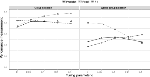
Figure 1: Effect of the tuning parameter $c$ on variable selection. The tuning parameter $c$ is varied from $0$ to $0.4$. Under each value of $c$, the best $\lambda$ value, which maximizes the likelihood of the test data set, is selected to generate the sparse model. Group (left) and within-group (right) selection performances are then evaluated using measures of recall, precision and $F_{1}$ based on 100 replications. Simulation setting: $n=100$, $p=100$, $p_{r}=4$, $q=40$, $q_{r}=4$, $m=500$, $\theta=0.025$, $\rho=0.4$.

5.2 Evaluation of the penalized likelihood approach for selecting covariates affecting the microbiome composition

To evaluate the variable selection performance of the proposed sparse penalized likelihood approach with group $\ell_{1}$ penalty, we first simulate the count data using the exponential growth model with $n=100$, $p=100$, $p_{r}=4$, $q=40$, $q_{r}=4$, $m=1000$, $\theta=0.025$, and $\rho=0.4$, totaling $4000$ variables. We compare the results to the corresponding penalized estimation of the DM model using only the $\ell_{1}$ penalty function and two other sparse group $\ell_{1}$ estimations based on multinomial or Dirichlet regression. In sparse multinomial regression, we use the multinomial model for count data and the link function is given by (12). We set $\beta_{10}=0$ to make the coefficients identifiable. In sparse Dirichlet regression, instead of modeling the counts directly, we model the proportions using the Dirichlet distribution and the link function is the same as that of the DM regression. Since the count data contain zeros, we add 0.5 to the cells with 0 counts. We also include results from the LRT based univariate testing procedure for group selection controlling the false discovery rate (FDR) at 0.05.

We measure the selection performance using

$$\mathrm{recall}=\frac{\mathrm{TP}}{\mathrm{TP}+\mathrm{FN}},\qquad\mathrm{precision}=\frac{\mathrm{TP}}{\mathrm{TP}+\mathrm{FP}},\qquad F_{1}=2\cdot\frac{\mathrm{precision}\cdot\mathrm{recall}}{\mathrm{precision}+\mathrm{recall}},$$

where $\mathrm{TP}$, $\mathrm{FN}$ and $\mathrm{FP}$ are true positives, false negatives and false positives, respectively, and $F_{1}$ is an overall measure, which weights the precision and recall equally. The averages of these measures are reported based on $100$ replications.

To select the best tuning parameter values, we simulate an independent test data set of $n/2$ samples. We then run the penalized procedure over the training data set and re-estimate the selected coefficients using an unpenalized procedure (“nlm” function in R). The log-likelihood of the test data set is calculated based on the re-estimated coefficients and the tuning parameter is selected to maximize the log-likelihood over the test data set. We choose the tuning parameter $c$ from the set $\{0,0.05,0.1,0.2,0.4\}$. Figure 1 shows that a small $c$ is sufficient to identify the groups efficiently, while further increase of $c$ only improves the group selection marginally. On the other hand, within-group selection exhibits a unimode pattern indicating slight grouping could lead to better identification of within-group elements. In the following simulations, we tune both $c$ and $\lambda$ to achieve the maximum likelihood values in the test data sets.

Table 1 shows the simulation results. The sparse group $\ell_{1}$ penalized DM regression has a much higher precision rate in group selection than the corresponding $\ell_{1}$ penalized procedure, while both achieve similar recall rates, demonstrating the gain from including the group $\ell_{1}$ penalty in the regularization. Interestingly, the sparse group penalized DM regression also performs better in within-group selection, as shown by a higher recall rate and $F_{1}$, indicating better group selection could also facilitate better overall variable selection. Compared to models based on the sparse Dirichlet regression and multinomial regression, the DM model performs

= Sparse group $\bolds{\ell_{1}}$ penalization $\bolds{\ell_{1}}$ penalization Within-group Group Within-group Group Model R P F R P F R P F R P F Exponential growth, $p=100,q_{r}=4,\theta=0.025$ DM 0.59 0.70 0.59 0.86 0.92 0.87 0.42 0.76 0.48 0.88 0.68 0.70 (0.23) (0.23) (0.18) (0.23) (0.16) (0.18) (0.21) (0.23) (0.18) (0.22) (0.29) (0.22) D 0.48 0.73 0.52 0.83 0.89 0.82 0.36 0.82 0.45 0.82 0.77 0.72 (0.23) (0.23) (0.20) (0.26) (0.18) (0.21) (0.20) (0.21) (0.19) (0.26) (0.27) (0.23) M 0.46 0.72 0.50 0.82 0.85 0.79 0.36 0.76 0.44 0.84 0.70 0.69 (0.23) (0.26) (0.21) (0.27) (0.24) (0.25) (0.19) (0.24) (0.18) (0.26) (0.28) (0.24) LRT – – – 0.96 0.54 0.66 – – – 0.96 0.54 0.66 – – – (0.11) (0.21) (0.16) – – – (0.11) (0.21) (0.16)

Table 1: Comparison of sparse group $\ell_{1}$ and $\ell_{1}$ penalized procedures for variable selection under Dirichlet-multinomial (DM),Dirichlet (D) and multinomial (M) regression models. The selection performance, both group selection andwithin-group selection, is evaluated using recall rate (R), precision rate (P) and $F_{1}$ (F), all averaged over 100 runs(standard deviation in parenthesis). The selection based on a univariate likelihood ratio test (LRT) at FDR${}={}$0.05 is also indicated

better in variable selection, especially for within-group selection, suggesting the DM model is more appropriate than multinomial or Dirichlet models when the counts exhibit overdispersion. The Dirichlet model performs slightly better than the multinomial model. At 5% FDR, the LRT based univariate testing procedure selects far more variables than these penalized procedures, yielding a higher recall rate but a much worse precision rate.

5.3 Effects of overdispersion and model misspecification

We further investigate the effect of overdispersion and simulate the count data with different degrees of overdispersion and present the results in Figure 2. We observe that larger overdispersion makes the selection more difficult for all three models, as shown by smaller $F_{1}$ values. When the data have slight overdispersion ($\theta=0.005$), the selection performances of the three models are similar. On the other hand, when the data have much overdispersion ($\theta=0.1$), DM performs much better than the other two models in terms of both group selection and within-group selection. Therefore, modeling overdispersion can lead to power gains in identifying relevant variables if the data are overdispersed.

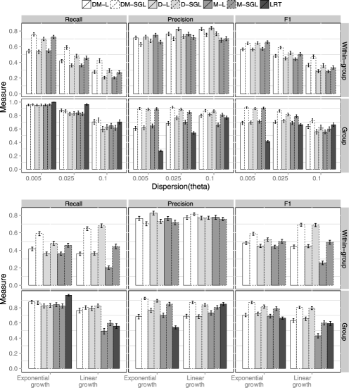
Figure 2: Effects of overdispersion (top panel) and model-misspecification (bottom panel) on the performance of three different models and methods. DM-SGL: sparse group $\ell_{1}$ penalized Dirichlet-multinomial model; DM-L: $\ell_{1}$ penalized Dirichlet-multinomial model; M-SGL: sparse group $\ell_{1}$ penalized multinomial model; M-L: $\ell_{1}$ penalized multinomial model; D-SGL: sparse group $\ell_{1}$ penalized Dirichlet model; D-L: $\ell_{1}$ penalized Dirichlet model. For each bar, mean${}\pm{}$standard error is presented based on 100 replications.

To assess the sensitivity to model misspecification, we simulate the counts using the linear growth model instead and compare the results with the exponential growth model (see Figure 2). Interestingly, both the Dirichlet and DM model are very robust to model misspecification and their selection performances do not decrease significantly. On the other hand, the multinomial model suffers a large performance loss with the $F_{1}$ measure for group selection decreasing from $0.79$ to $0.56$. We also study the effect of the total counts for each sample (data not shown). Even increasing the total count by 10 folds, the DM model is still better than the proportion based Dirichlet model. Therefore, even though we have much deeper sequencing of the microbiome that results in larger counts for each sample, using the DM model can still lead to improved performance over the model that considers only the proportions.

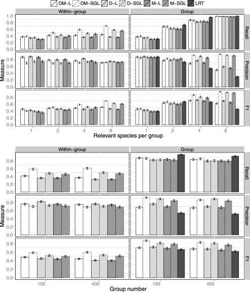
Figure 3: Effects of the number of relevant taxa (top panel) and the number of the covariates (bottom panel) on the performances of several models and methods. DM-SGL: sparse group $\ell_{1}$ penalized Dirichlet-multinomial model; DM-L: $\ell_{1}$ penalized Dirichlet-multinomial model; M-SGL: sparse group $\ell_{1}$ penalized multinomial model; M-L: $\ell_{1}$ penalized multinomial model; D-SGL: sparse group $\ell_{1}$ penalized Dirichlet model; D-L: $\ell_{1}$ penalized Dirichlet model. For each bar, mean${}\pm{}$standard error is presented based on 100 replications.

5.4 Effects of the number of the covariates and the relevant taxa

We next study the effect of the number of relevant taxa in each group on the performance of different models and present the results in Figure 3. When each relevant group contains only one relevant taxon, the grouping is not very helpful, so the sparse group regularized DM model and $\ell_{1}$ regularized DM model do not differ much in selecting the relevant groups. When the relevant group contains $8$ relevant taxa, variable grouping becomes much more important and the sparse group regularized DM model performs much better than the $\ell_{1}$ penalized DM. The group penalized multinomial and Dirichlet regression models, on the other hand, select groups as well as the DM regression model, since the grouping effect is much stronger.

Figure 3 also shows the results when we increase the dimension of covariates to 400 ($16\mbox{,}000$ variables in total). Increase of the dimension does not deteriorate the variable selection performance, demonstrating the efficiency of our method in handling high-dimensional data.

6 Associating nutrient intake with the human gut microbiome composition

Diet strongly affects the human health, partly by modulating gut microbial community composition. Wu et al. (2011) studied the habitual diet effect on the human gut microbiome, where a cross-section of 98 healthy volunteers were enrolled in the study. Diet information was collected using a food frequency questionnaire (FFQ) and was then converted to nutrient intake values of 214 micronutrients. Nutrient intake was further normalized using the residual method to adjust for caloric intake and was standardized to have mean 0 and standard deviation 1. Since some nutrient measurements were almost identical, we used only one representative for these highly correlated nutrients (correlation $\rho>0.9$), resulting in 118 representative nutrients. Stool samples were collected and DNA samples were analyzed by the 454$/$Roche pyrosequencing of 16S rDNA gene segments of the V1–V2 region. The pyrosequences were denoised prior to taxonomic assignment, yielding an average of $9265\pm 3864$ (SD) reads per sample. The denoised sequences were then analyzed by the QIIME pipeline [Caporaso et al. (2010)] with the default parameter settings. The OTU table contained 3068 OTUs (excluding the singletons) and these OTUs can be further combined into 127 genera. We studied 30 relatively common genera that appeared in at least 25 subjects. Finally, we had the count matrix ${\mathbf{Y}}_{98\times 30}$ and covariate matrix $X_{98\times 118}$. Our goal is to identify the micronutrients that are associated with the gut microbiomes and the specific genera that the selected nutrients affect.

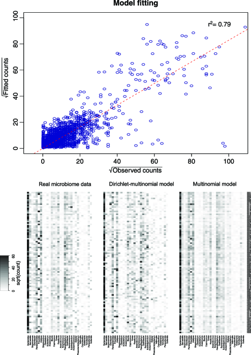
Figure 4: Model fit using the variables selected by the sparse group $l_{1}$ penalized DM model. Top plot: square root of the fitted counts versus square root of the observed counts based on the DM model with the selected nutrients; bottom plots: observed counts and simulated counts produced by the fitted sparse DM model and multinomial model.

= Row: taxon; column: nutrient – $-0.03$ $-0.08$ 0.09 $-0.08$ $-0.10$ $-0.02$ $0.02$ $0.10$ – $-0.03$ $-$0.32 – $-0.33$ – – – $0.22$ – – – – $-$0.38 – – – – – – – – $-0.29$ – – $-0.01$ $-0.08$ 0.13 $-0.07$ – – – $0.02$ $-0.23$ – – – $0.23$ – – $0.36$ $0.63$ $-0.72$ – – – $-$0.19 $-0.04$ – 0.16 – – – – – – $0.05$ – – – – – – – – – – $0.16$ – – – – – $-0.08$ – – – $0.07$ – – $-0.02$ – – – – – – $-0.10$ – – – – $0.19$ – – – – – – – – – $0.02$ – – – – – – $-0.12$ $-0.12$ $0.14$ – – – – $-0.35$ – – – – – – $-$0.26 – $-0.29$ – – – – – – – – Marginal $\bolds{p}$-value $4.5\times 10^{-3}$ $2.2\times 10^{-4}$ $8.4\times 10^{-4}$ $3.6\times 10^{-4}$ $1.1\times 10^{-1}$ $6.0\times 10^{-3}$ $9.5\times 10^{-6}$ $2.7\times 10^{-3}$ $5.9\times 10^{-3}$ $5.8\times 10^{-2}$ $5.2\times 10^{-3}$ Bootstrap selection probability 0.50 $0.93$ $0.72$ 0.94 $0.35$ $0.67$ $0.43$ $0.58$ $0.92$ $0.61$ $0.60$

Table 2: Estimated regression coefficients from the sparse group $\ell_{1}$ penalized DM regression for the diet-gut microbiome data.The exponentiation of a given coefficient can be interpreted as the factor of change in proportion of a taxon whena given nutrient changes by one unit while other nutrients remain constant. Columns 1–11 represent the selected nutrients: Polyunsaturated fat, Methionine, Sucrose, Animal Protein, Vitamin E-Food Fortification, Maltose, Added Germ from wheats, Choline-Phosphatidylcholine, Taurine, Naringenin-flavanone and Eriodictyol-flavonone. Rows 1–13 represent the selectedbacteria taxa: Bacteroides, Barnesiella, Odoribacter, Parabacteroides, Prevotella, Alistipes, Coprococcus, Faecalibacterium,Oscillibacter, Ruminococcus, Subdoligranulum, Phascolarctobacterium and Parasutterella. The marginal $p$-valuebased on the LRT and the bootstrap selection probability of each of the selected nutrients are also shown

We applied the sparse group $\ell_{1}$ penalized DM regression to this data set. We used the BIC to select the tuning parameters. The final DM model selected 11 nutrients and 13 associated genera. We refit the DM regression model using the selected variables and obtained the maximum likelihood estimates of the coefficients. We compared the fitted counts (total count${}\times{}$fitted proportion) against the observed counts in Figure 4 (top panel). The model fits the data quite well with $r^{2}=0.79$. Table 2 shows the MLEs of the regression coefficients for the selected nutrients and genera. Except for Methionine (second column), the coefficients are not too small. Since the nutrient measurements are standardized, the exponentiation of a given coefficient can be interpreted as the factor of change in proportion of a taxon when a given nutrient changes by one unit while other nutrients remain constant. The marginal $p$-value based on the LRT for each of the selected nutrients is also shown in this table. Except for Vitamin E and Eriodictyol, these selected nutrients all showed a significant marginal association with the gut microbiome.

To further assess the relevance of the nutrients selected, we used the bootstrap to analyze the stability of the selected nutrients [Bach (2008)]. Specifically, we took 100 bootstrap samples and for each sample we ran our algorithm to select the nutrients. Since some nutrients are highly correlated, we expect that highly correlated nutrients (if the correlation is greater than 0.75) can be selected in different bootstrap samples; we define the bootstrap selection probability of a given nutrient as the number of times that this nutrient or its correlated nutrients were selected. Table 2 shows the bootstrap probabilities of the nutrients that were selected by the sparse DM regression, indicating quite stable selection of most of the selected microbiome-associated nutrients. Vitamin E had the least stable selection over the 100 bootstrap samples.

The identified nutrient-taxon associations are visualized in a bipartite graph shown in Figure 5, where the genera and nutrients are depicted with circles and hexagons, respectively. These results further confirmed the findings of Wu et al. (2011), where they found the human gut microbiome can be clustered into two enterotypes characterized by Prevotella and Bacteroides, respectively, and the Prevotella enterotype is associated with a high carbohydrate diet while the Bacteroides enterotype is associated with a high protein/fat/choline diet. Figure 5 shows that two carbohydrates, Maltose and Sucrose, are positively associated with Prevotella and negatively associated with Bacteroides, while animal proteins are positively associated with Bacteroides, Parabacteroides and Alistipes, the three genera mostly enriched in the Bacteroides enterotype. Choline is positively associated with Bacteroides and negatively associated with Prevotella. Polyunsaturated fat is strongly associated with Alistipes, Odoribacter, Barnesiella and Parasutterella, indicating the large effect of fat on the human microbiome.

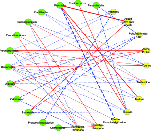
Figure 5: Association of nutrients with human gut microbial taxa identified by the sparse group $\ell_{1}$ regularized DM model. We use a bipartite graph to visualize the selected nutrients and their associated genera based on sparse group $\ell_{1}$ penalized DM regression. Circle: genus; hexagon: nutrient; solid line: positive correlation; dashed line: negative correlation. The thickness of the line represents the association strength.

The DM model also identified several other associations that are worth further investigation. For example, we found that Naringenin (flavanone) was positively associated with Faecalibacterium, an anti-inflammatory commensal bacterium identified by gut microbiota analysis of Crohn’s disease patients [Sokol et al. (2008)]. If the association is validated, diet with high Naringenin (e.g., Orange, Grapefruit) can be beneficial for patients with Crohn’s disease.

As a comparison, we also ran the sparse group $\ell_{1}$ penalized multinomial or Dirichlet regression models and the identified nutrient-genus associations showed significant overlap with those from the DM regression model. However, the interpretability of the DM regression model was the best. To further demonstrate the advantage of the DM model, we simulated taxa counts for each individual based on the fitted models and the observed total taxa counts. The bottom plot of Figure 4 shows that the simulated counts produced by the fitted sparse DM model resemble the observed counts better than those from the sparse multinomial model, where the simulated counts are apparently over-smoothed. This indicates the importance of considering the overdispersion in modeling the gut microbiome data. We also performed the LRT based univariate testing procedure. At FDR${}={}$0.05, the LRT identified 13 nutrients, 8 of which are also identified or highly correlated with the nutrients identified by the sparse group $\ell_{1}$ penalized DM model.

7 Discussion

We have proposed a sparse group $\ell_{1}$ penalized estimation for the DM regression in order to select covariates associated with the microbiome composition. The sparse group $\ell_{1}$ penalty encourages both group-level and within-group sparsity, with which we can select the relevant taxa associated with the selected covariates. We have performed extensive simulations to evaluate our proposed penalized estimation procedure for both group and within-group selections. We demonstrated the procedure with a real data set on associating nutrient intakes with gut microbiome composition and confirmed the major findings in Wu et al. (2011).

In our penalized likelihood estimation of the DM model, we use a combination of group $\ell_{1}$ and individual $\ell_{1}$ penalties, which result in a convex and separable (in groups of parameters) penalty function. This property facilitates the application of the general coordinate gradient descent method of Tseng and Yun (2008) to implement an efficient optimization algorithm. In each iteration, we have a closed form solution for a block update. For a given set of the sparsity tuning parameters, our algorithm is fully automatic and does not require the specification of an algorithmic tuning parameter to ensure convergence. For example, it took about 3 minutes on a standard laptop (Core i5, 2G memory) to finish the analysis of the real data set using an R implementation of the algorithm (available at http://statgene.med.upenn.edu/). Besides the sparse $l_{1}$ group penalty, other group penalty functions such as the sup-norm penalty in Zhang et al. (2008) and the composite absolute penalties in Zhao, Rocha and Yu (2009) can also be used in the setup of the Dirichlet multinomial regression. However, efficient implementation of the optimization problems with these penalty functions is challenging.

In microbiome data analysis literature, one commonly used approach is to normalize the counts into proportions and perform statistical analysis using the proportions. However, by converting into the proportions, the variation associated with the multinomial sampling process is lost. In 16S rRNA sequencing, the sequencing depths (total counts) for samples can vary up to 10-fold. Obviously, the accuracy of the proportion estimates under sequencing depth of $500$ reads is very different from that of $10\mbox{,}000$ reads. As shown in our simulations, modeling counts directly can result in gain of power in selecting relevant variables even when the number of sequence reads is very large. Another problem associated with proportions is the existence of numerous zeros in the taxa count data. Many proportion based approaches require taking logarithms of the proportions, which is problematic for the zero proportions. To circumvent this problem, either a pseudo count (e.g., 0.5) is added to these zero counts before converting into proportions or an arbitrary small proportion is substituted for these zero proportions. The effects of creating pseudo counts have not been evaluated thoroughly when the data contain excessive zeros.

Besides overdispersion, the taxa count data can also exhibit zero-inflation [Barry and Welsh (2002)], where the count data contain more zeros than expected from the DM model. How to model the microbiome count data that allows overdispersion, zero-inflation and possibly the phylogenetic correlations among the taxa is an important future research topic. The multilevel zero-inflated DM regression model for overdispersed count data with extra zeros [Moghimbeigi et al. (2008), Lee et al. (2006)] can potentially provide a solution to this problem. Another problem associated with the DM model is its inflexibility in modeling the covariance structure among the taxa counts. The multinomial model for counts compounded by a logistic normal model [Aitchison (1982)] for proportions provides a possible solution. This needs to be investigated further.

Appendix

Theorem 1.

Letting ${\mathbf{b}},{\mathbf{x}}\in\mathbb{R}^{n}$, $\lambda_{1},\lambda_{2},c$ are nonnegative constants and ${\mathbf{x}}^{0}$ is the minimizer of the following function:

$$f({\mathbf{x}})=\tfrac{1}{2}{\mathbf{x}}^{T}{\mathbf{x}}+{\mathbf{b}}^{T}{\mathbf{x}}+c+\lambda_{1}\|{\mathbf{x}}\|_{2}+\lambda_{2}\|{\mathbf{x}}\|_{1},$$ (13)

then ${\mathbf{x}}^{0}_{S}={\mathbf{0}}$ and

$${\mathbf{x}}^{0}_{\bar{S}}=\arg\min_{{\mathbf{x}}_{\bar{S}}}\bigl{\{}\tfrac{1}{2}{\mathbf{x}}^{T}_{\bar{S}}{\mathbf{x}}_{\bar{S}}+\bigl{(}{\mathbf{b}}_{\bar{S}}-\lambda_{2}\operatorname{sgn}({\mathbf{b}}_{\bar{S}})\bigr{)}^{T}{\mathbf{x}}_{\bar{S}}+c+\lambda_{1}\|{\mathbf{x}}_{\bar{S}}\|_{2}\bigr{\}},$$

where $S=\{i\in\{1,\ldots,n\}||b_{i}|<\lambda_{2}\}$ and $\bar{S}=\{1,\ldots,n\}\setminus S$ and $\operatorname{sgn}(\cdot)$ is the sign function.

We prove ${\mathbf{x}}^{0}_{S}={\mathbf{0}}$ by contradiction. If $x^{0}_{i}\neq 0$ $(i\in S)$, then we can construct a new ${\mathbf{x}}^{1}$ with $x^{1}_{i}=0$ and other components being the same as ${\mathbf{x}}^{0}$. Clearly, $\frac{1}{2}{{\mathbf{x}}^{1}}^{T}{\mathbf{x}}^{1}+{\mathbf{b}}^{T}{\mathbf{x}}^{1}+c+\lambda_{2}\|{\mathbf{x}}^{1}\|_{1}<\frac{1}{2}{{\mathbf{x}}^{0}}^{T}{\mathbf{x}}^{0}+{\mathbf{b}}^{T}{\mathbf{x}}^{0}+c+\lambda_{2}\|{\mathbf{x}}^{0}\|_{1}$ and $\lambda_{1}\|{\mathbf{x}}^{1}\|_{2}<\lambda_{1}\|{\mathbf{x}}^{0}\|_{2}$. The former is due to the fact that $\frac{1}{2}(x_{i}^{0})^{2}+b_{i}x_{i}^{0}+\lambda_{2}|x_{i}^{0}|>0$ for $|b_{i}|<\lambda_{2}$. Hence, ${\mathbf{x}}^{0}$ is not the minimizer of $f({\mathbf{x}})$, which is contradictory. Therefore, ${\mathbf{x}}^{0}_{S}={\mathbf{0}}$.

To prove the second part, we note that $x_{i}^{0}$ must be either $0$ or have an opposite sign of $b_{i}$ for $i\in\{1,\ldots,n\}$. So the minimization of ${\mathbf{f}}({\mathbf{x}})$ is equivalent to minimizing

$$f^{*}({\mathbf{x}})=\tfrac{1}{2}{\mathbf{x}}^{T}{\mathbf{x}}+\bigl{(}{\mathbf{b}}-\lambda_{2}\operatorname{sgn}({\mathbf{b}})\bigr{)}^{T}{\mathbf{x}}+c+\lambda_{1}\|{\mathbf{x}}\|_{2},$$

subject to

$$\operatorname{sgn}(x_{i})=-\operatorname{sgn}(b_{i})\quad\mbox{or}\quad x_{i}=0.$$

Since ${\mathbf{x}}^{0}_{S}={\mathbf{0}}$, we can restrict the minimization over only ${\mathbf{x}}_{\bar{S}}$,

$$f^{*}({\mathbf{x}}_{\bar{S}})=\tfrac{1}{2}{\mathbf{x}}_{\bar{S}}^{T}{\mathbf{x}}_{\bar{S}}+\bigl{(}{\mathbf{b}}_{\bar{S}}-\lambda_{2}\operatorname{sgn}({\mathbf{b}}_{\bar{S}})\bigr{)}^{T}{\mathbf{x}}_{\bar{S}}+c+\lambda_{1}\|{\mathbf{x}}_{\bar{S}}\|_{2},$$ (14)

subject to

$$\operatorname{sgn}(x_{i})=-\operatorname{sgn}(b_{i})\quad\mbox{or}\quad x_{i}=0\qquad(i\in\bar{S}).$$

Since ${\mathbf{x}}^{0}_{\bar{S}}$ is the minimizer of $f^{*}({\mathbf{x}}_{\bar{S}})$ without the constraint, the sign of ${\mathbf{x}}^{0}_{\bar{S}}$ should be the opposite of the sign of $({\mathbf{b}}_{\bar{S}}-\lambda_{2}\operatorname{sgn}({\mathbf{b}}_{\bar{S}}))$. Because $|b_{i}|\geq\lambda_{2}$ for $i\in\bar{S}$, the sign of $({\mathbf{b}}_{\bar{S}}-\lambda_{2}\operatorname{sgn}({\mathbf{b}}_{\bar{S}}))$ is the same as ${\mathbf{b}}_{\bar{S}}$. So the sign of ${\mathbf{x}}^{0}_{\bar{S}}$ is the opposite of that of ${\mathbf{b}}_{\bar{S}}$. Therefore, ${\mathbf{x}}^{0}_{\bar{S}}$ satisfies the constraint.

Using simple variable substitution, we have the following corollary.

Corollary 1.

Letting ${\mathbf{b}},\bolds{\beta},{\mathbf{d}}\in\mathbb{R}^{n}$, $\lambda_{1},\lambda_{2},c$ are nonnegative constants and ${\mathbf{d}}^{0}$ is the minimizer of the following function,

$$f({\mathbf{d}})=\tfrac{1}{2}{\mathbf{d}}^{T}{\mathbf{d}}+{\mathbf{b}}^{T}{\mathbf{d}}+c+\lambda_{1}\|\bolds{\beta}+{\mathbf{d}}\|_{2}+\lambda_{2}\|\bolds{\beta}+{\mathbf{d}}\|_{1},$$ (15)

then ${\mathbf{d}}^{0}_{S}=-\bolds{\beta}_{S}$ and

$${\mathbf{d}}^{0}_{\bar{S}}=\arg\min_{{\mathbf{d}}_{\bar{S}}}\biggl{\{}\frac{1}{2}{\mathbf{d}}^{T}_{\bar{S}}{\mathbf{d}}_{\bar{S}}+\bigl{(}{\mathbf{b}}_{\bar{S}}-\lambda_{2}\operatorname{sgn}({\mathbf{b}}_{\bar{S}}-\bolds{\beta}_{\bar{S}})\bigr{)}^{T}{\mathbf{d}}_{\bar{S}}+c+\lambda_{1}\|{\mathbf{d}}_{\bar{S}}+\bolds{\beta}_{\bar{S}}\|_{2}\biggr{\}},$$

where $S=\{i\in\{1,\ldots,n\}||b_{i}-\beta_{i}|<\lambda_{2}\}$, $\bar{S}=\{1,\ldots,n\}\setminus S$ and $\operatorname{sgn}(\cdot)$ is the sign function.

References

- Aitchison (1982) {barticle}[mr] \bauthor\bsnmAitchison, \bfnmJ.\binitsJ. (\byear1982). \btitleThe statistical analysis of compositional data. \bjournalJ. R. Stat. Soc. Ser. B Stat. Methodol. \bvolume44 \bpages139–177. \bidissn=0035-9246, mr=0676206 \bptokimsref \endbibitem
- Bach (2008) {bmisc}[author] \bauthor\bsnmBach, \bfnmF. R.\binitsF. R. (\byear2008). \bhowpublishedBolasso: Model consistent Lasso estimation through the bootstrap. In ICML’08: Proceedings of the 25th International Conference on Machine Learning 33–40. ACM, New York. \bptokimsref \endbibitem
- Bäckhed et al. (2005) {barticle}[pbm] \bauthor\bsnmBäckhed, \bfnmFredrik\binitsF., \bauthor\bsnmLey, \bfnmRuth E.\binitsR. E., \bauthor\bsnmSonnenburg, \bfnmJustin L.\binitsJ. L., \bauthor\bsnmPeterson, \bfnmDaniel A.\binitsD. A. and \bauthor\bsnmGordon, \bfnmJeffrey I.\binitsJ. I. (\byear2005). \btitleHost-bacterial mutualism in the human intestine. \bjournalScience \bvolume307 \bpages1915–1920. \biddoi=10.1126/science.1104816, issn=1095-9203, pii=307/5717/1915, pmid=15790844 \bptokimsref \endbibitem
- Barry and Welsh (2002) {barticle}[author] \bauthor\bsnmBarry, \bfnmS.\binitsS. and \bauthor\bsnmWelsh, \bfnmA.\binitsA. (\byear2002). \btitleGeneralized additive modelling and zero inflated count data. \bjournalEcological Modelling \bvolume157 \bpages179–188. \bptokimsref \endbibitem
- Benson et al. (2010) {barticle}[author] \bauthor\bsnmBenson, \bfnmA. K.\binitsA. K., \bauthor\bsnmKelly, \bfnmS. A.\binitsS. A., \bauthor\bsnmLegge, \bfnmR.\binitsR., \bauthor\bsnmMa, \bfnmF.\binitsF., \bauthor\bsnmLow, \bfnmS. J.\binitsS. J., \bauthor\bsnmKim, \bfnmJ.\binitsJ., \bauthor\bsnmZhang, \bfnmM.\binitsM., \bauthor\bsnmOh, \bfnmP. L.\binitsP. L., \bauthor\bsnmNehrenberg, \bfnmD.\binitsD., \bauthor\bsnmHua, \bfnmK.\binitsK. \betalet al. (\byear2010). \btitleIndividuality in gut microbiota composition is a complex polygenic trait shaped by multiple environmental and host genetic factors. \bjournalProc. Natl. Acad. Sci. USA \bvolume107 \bpages18933–18938. \bptokimsref \endbibitem
- Caporaso et al. (2010) {barticle}[author] \bauthor\bsnmCaporaso, \bfnmJ. G.\binitsJ. G., \bauthor\bsnmKuczynski, \bfnmJ.\binitsJ., \bauthor\bsnmStombaugh, \bfnmJ.\binitsJ., \bauthor\bsnmBittinger, \bfnmK.\binitsK., \bauthor\bsnmBushman, \bfnmF. D.\binitsF. D., \bauthor\bsnmCostello, \bfnmE. K.\binitsE. K., \bauthor\bsnmFierer, \bfnmN.\binitsN., \bauthor\bsnmPeña, \bfnmA. G.\binitsA. G., \bauthor\bsnmGoodrich, \bfnmJ. K.\binitsJ. K., \bauthor\bsnmGordon, \bfnmJ. I.\binitsJ. I. \betalet al. (\byear2010). \btitleQIIME allows analysis of high-throughput community sequencing data. \bjournalNature Methods \bvolume7 \bpages335–336. \bptokimsref \endbibitem
- Friedman, Hastie and Tibshirani (2010) {bmisc}[author] \bauthor\bsnmFriedman, \bfnmJ.\binitsJ., \bauthor\bsnmHastie, \bfnmT.\binitsT. and \bauthor\bsnmTibshirani, \bfnmR.\binitsR. (\byear2010). \bhowpublishedA note on the group lasso and a sparse group lasso. Preprint. Available at arXiv:\arxivurl1001.0736. \bptokimsref \endbibitem
- Lee et al. (2006) {barticle}[mr] \bauthor\bsnmLee, \bfnmAndy H.\binitsA. H., \bauthor\bsnmWang, \bfnmKui\binitsK., \bauthor\bsnmScott, \bfnmJane A.\binitsJ. A., \bauthor\bsnmYau, \bfnmKelvin K. W.\binitsK. K. W. and \bauthor\bsnmMcLachlan, \bfnmGeoffrey J.\binitsG. J. (\byear2006). \btitleMulti-level zero-inflated Poisson regression modelling of correlated count data with excess zeros. \bjournalStat. Methods Med. Res. \bvolume15 \bpages47–61. \biddoi=10.1191/0962280206sm429oa, issn=0962-2802, mr=2225145 \bptokimsref \endbibitem
- Legendre and Legendre (2002) {bbook}[author] \bauthor\bsnmLegendre, \bfnmP.\binitsP. and \bauthor\bsnmLegendre, \bfnmL.\binitsL. (\byear2002). \btitleNumerical Ecology, \bedition2nd ed. \bpublisherElsevier, \blocationAmsterdam. \bptokimsref \endbibitem
- Matsen, Kodner and Armbrust (2010) {barticle}[pbm] \bauthor\bsnmMatsen, \bfnmFrederick A.\binitsF. A., \bauthor\bsnmKodner, \bfnmRobin B.\binitsR. B. and \bauthor\bsnmArmbrust, \bfnmE. Virginia\binitsE. V. (\byear2010). \btitlepplacer: Linear time maximum-likelihood and Bayesian phylogenetic placement of sequences onto a fixed reference tree. \bjournalBMC Bioinformatics \bvolume11 \bpages538. \biddoi=10.1186/1471-2105-11-538, issn=1471-2105, pii=1471-2105-11-538, pmcid=3098090, pmid=21034504 \bptokimsref \endbibitem
- McArdle (2001) {barticle}[author] \bauthor\bsnmMcArdle, \bfnmB. H.\binitsB. H. (\byear2001). \btitleFitting multivariate models to community data: A comment on distance-based redundancy analysis. \bjournalEcology \bvolume82 \bpages290–297. \bptokimsref \endbibitem
- Meier, van de Geer and Bühlmann (2008) {barticle}[mr] \bauthor\bsnmMeier, \bfnmLukas\binitsL., \bauthor\bparticlevan de \bsnmGeer, \bfnmSara\binitsS. and \bauthor\bsnmBühlmann, \bfnmPeter\binitsP. (\byear2008). \btitleThe group Lasso for logistic regression. \bjournalJ. R. Stat. Soc. Ser. B Stat. Methodol. \bvolume70 \bpages53–71. \biddoi=10.1111/j.1467-9868.2007.00627.x, issn=1369-7412, mr=2412631 \bptokimsref \endbibitem
- Moghimbeigi et al. (2008) {barticle}[mr] \bauthor\bsnmMoghimbeigi, \bfnmAbbas\binitsA., \bauthor\bsnmEshraghian, \bfnmMohammed Reza\binitsM. R., \bauthor\bsnmMohammad, \bfnmKazem\binitsK. and \bauthor\bsnmMcArdle, \bfnmBrian\binitsB. (\byear2008). \btitleMultilevel zero-inflated negative binomial regression modeling for over-dispersed count data with extra zeros. \bjournalJ. Appl. Stat. \bvolume35 \bpages1193–1202. \biddoi=10.1080/02664760802273203, issn=0266-4763, mr=2522147 \bptokimsref \endbibitem
- Mosimann (1962) {barticle}[mr] \bauthor\bsnmMosimann, \bfnmJames E.\binitsJ. E. (\byear1962). \btitleOn the compound multinomial distribution, the multivariate -distribution, and correlations among proportions. \bjournalBiometrika \bvolume49 \bpages65–82. \bidissn=0006-3444, mr=0143299 \bptokimsref \endbibitem
- Peng et al. (2010) {barticle}[mr] \bauthor\bsnmPeng, \bfnmJie\binitsJ., \bauthor\bsnmZhu, \bfnmJi\binitsJ., \bauthor\bsnmBergamaschi, \bfnmAnna\binitsA., \bauthor\bsnmHan, \bfnmWonshik\binitsW., \bauthor\bsnmNoh, \bfnmDong-Young\binitsD.-Y., \bauthor\bsnmPollack, \bfnmJonathan R.\binitsJ. R. and \bauthor\bsnmWang, \bfnmPei\binitsP. (\byear2010). \btitleRegularized multivariate regression for identifying master predictors with application to integrative genomics study of breast cancer. \bjournalAnn. Appl. Stat. \bvolume4 \bpages53–77. \biddoi=10.1214/09-AOAS271, issn=1932-6157, mr=2758084 \bptnotecheck year\bptokimsref \endbibitem
- Schloss et al. (2009) {barticle}[author] \bauthor\bsnmSchloss, \bfnmP. D.\binitsP. D., \bauthor\bsnmWestcott, \bfnmS. L.\binitsS. L., \bauthor\bsnmRyabin, \bfnmT.\binitsT., \bauthor\bsnmHall, \bfnmJ. R.\binitsJ. R., \bauthor\bsnmHartmann, \bfnmM.\binitsM., \bauthor\bsnmHollister, \bfnmE. B.\binitsE. B., \bauthor\bsnmLesniewski, \bfnmR. A.\binitsR. A., \bauthor\bsnmOakley, \bfnmB. B.\binitsB. B., \bauthor\bsnmParks, \bfnmD. H.\binitsD. H., \bauthor\bsnmRobinson, \bfnmC. J.\binitsC. J. \betalet al. (\byear2009). \btitleIntroducing mothur: Open-source, platform-independent, community-supported software for describing and comparing microbial communities. \bjournalApplied and Environmental Microbiology \bvolume75 \bpages7537–7541. \bptokimsref \endbibitem
- Sokol et al. (2008) {barticle}[author] \bauthor\bsnmSokol, \bfnmH.\binitsH., \bauthor\bsnmPigneur, \bfnmB.\binitsB., \bauthor\bsnmWatterlot, \bfnmL.\binitsL., \bauthor\bsnmLakhdari, \bfnmO.\binitsO., \bauthor\bsnmBermúdez-Humarán, \bfnmL. G.\binitsL. G., \bauthor\bsnmGratadoux, \bfnmJ. J.\binitsJ. J., \bauthor\bsnmBlugeon, \bfnmS.\binitsS., \bauthor\bsnmBridonneau, \bfnmC.\binitsC., \bauthor\bsnmFuret, \bfnmJ. P.\binitsJ. P., \bauthor\bsnmCorthier, \bfnmG.\binitsG. \betalet al. (\byear2008). \btitleFaecalibacterium prausnitzii is an anti-inflammatory commensal bacterium identified by gut microbiota analysis of Crohn disease patients. \bjournalProc. Natl. Acad. Sci. USA \bvolume105 \bpages16731–16736. \bptokimsref \endbibitem
- Tseng and Yun (2008) {barticle}[mr] \bauthor\bsnmTseng, \bfnmPaul\binitsP. and \bauthor\bsnmYun, \bfnmSangwoon\binitsS. (\byear2008). \btitleA coordinate gradient descent method for nonsmooth separable minimization. \bjournalMath. Program. \bvolume117 \bpages387–423. \biddoi=10.1007/s10107-007-0170-0, issn=0025-5610, mr=2421312 \bptnotecheck year\bptokimsref \endbibitem
- Virgin and Todd (2011) {barticle}[pbm] \bauthor\bsnmVirgin, \bfnmHerbert W.\binitsH. W. and \bauthor\bsnmTodd, \bfnmJohn A.\binitsJ. A. (\byear2011). \btitleMetagenomics and personalized medicine. \bjournalCell \bvolume147 \bpages44–56. \biddoi=10.1016/j.cell.2011.09.009, issn=1097-4172, pii=S0092-8674(11)01063-4, pmid=21962506 \bptokimsref \endbibitem
- Wu et al. (2011) {barticle}[author] \bauthor\bsnmWu, \bfnmG. D.\binitsG. D., \bauthor\bsnmChen, \bfnmJ.\binitsJ., \bauthor\bsnmHoffmann, \bfnmC.\binitsC., \bauthor\bsnmBittinger, \bfnmK.\binitsK., \bauthor\bsnmChen, \bfnmY. Y.\binitsY. Y., \bauthor\bsnmKeilbaugh, \bfnmS. A.\binitsS. A., \bauthor\bsnmBewtra, \bfnmM.\binitsM., \bauthor\bsnmKnights, \bfnmD.\binitsD., \bauthor\bsnmWalters, \bfnmW. A.\binitsW. A., \bauthor\bsnmKnight, \bfnmR.\binitsR. \betalet al. (\byear2011). \btitleLinking long-term dietary patterns with gut microbial enterotypes. \bjournalScience \bvolume334 \bpages105–108. \bptokimsref \endbibitem
- Zhang et al. (2008) {barticle}[mr] \bauthor\bsnmZhang, \bfnmHao Helen\binitsH. H., \bauthor\bsnmLiu, \bfnmYufeng\binitsY., \bauthor\bsnmWu, \bfnmYichao\binitsY. and \bauthor\bsnmZhu, \bfnmJi\binitsJ. (\byear2008). \btitleVariable selection for the multicategory SVM via adaptive sup-norm regularization. \bjournalElectron. J. Stat. \bvolume2 \bpages149–167. \biddoi=10.1214/08-EJS122, issn=1935-7524, mr=2386091 \bptokimsref \endbibitem
- Zhao, Rocha and Yu (2009) {barticle}[mr] \bauthor\bsnmZhao, \bfnmPeng\binitsP., \bauthor\bsnmRocha, \bfnmGuilherme\binitsG. and \bauthor\bsnmYu, \bfnmBin\binitsB. (\byear2009). \btitleThe composite absolute penalties family for grouped and hierarchical variable selection. \bjournalAnn. Statist. \bvolume37 \bpages3468–3497. \biddoi=10.1214/07-AOS584, issn=0090-5364, mr=2549566 \bptokimsref \endbibitem