Narrowing the gap on heritability of common disease by direct estimation in case-control GWAS

Department of Statistics and Operations Research, Tel-Aviv University.

Summary paragraph

One of the major developments in recent years in the search for missing heritability of human phenotypes is the adoption of linear mixed-effects models (LMMs) to estimate heritability due to genetic variants which are not significantly associated with the phenotype(yang2010common, ). A variant of the LMM approach has been adapted to case-control studies and applied to many major diseases(Lee2011estimating, ; do2011web, ; lee2012estimating, ; lee2013estimation, ), successfully accounting for a considerable portion of the missing heritability. For example, for Crohn’s disease their estimated heritability was 22% compared to 50-60% from family studies. In this letter we propose to estimate heritability of disease directly by regression of phenotype similarities on genotype correlations, corrected to account for ascertainment. We refer to this method as genetic correlation regression (GCR). Using GCR we estimate the heritability of Crohn’s disease at 34% using the same data. We demonstrate through extensive simulation that our method yields unbiased heritability estimates, which are consistently higher than LMM estimates. Moreover, we develop a heuristic correction to LMM estimates, which can be applied to published LMM results. Applying our heuristic correction increases the estimated heritability of multiple sclerosis from 30%(lee2013estimation, ) to 52.6%.

Main text

The mystery of the “missing heritability” is a term commonly used to denote the gap between the expected heritability of many common diseases, as estimated by family and twin studies, and the overall additive (narrow-sense) heritability obtained by accumulating the effects of all single-nucleotide polymorphisms (SNPs) that have been found to be significantly associated with these conditions in genome-wide association studies (GWASs)(bloom2012finding, ; eichler2010missing, ; maher2008case, ; manolio2009finding, ). Many diseases which comprise a considerable portion of the health-care burden display such a gap, including type-1 and type-2 diabetes, bipolar disorder, schizophrenia, Alzheimer’s disease, multiple sclerosis and Parkinson’s disease.

Researchers have proposed several hypothetical solutions to this mystery. These theories include rare causative variants, which are undetected by the current GWAS methodology, common variants with small effects, which do not pass the significance threshold and are therefore unaccounted for, gene-gene and gene-environment interactions which are overlooked by the additive model assumed by the GWAS scheme, epigenetic effects and more(eichler2010missing, ; manolio2009finding, ; zuk2012mystery, ).

Clearly, different theories have major implications for our understanding of human disease, and also dictate different strategies for discovery of the underlying genetic causes of disease. For example, identifying rare variants requires a focus on deep sequencing(nielsen2011genotype, ), while detecting small effects of common variants requires increasing the sample sizes dramatically, or conducting massive meta-analyses(visscher2008sizing, ). Effective planning of genetic research can therefore only be guided by a satisfactory and well founded allocation of missing heritability to its various possible sources and causes. Additionally, accurate estimates of heritability can facilitate better personalized genetic risk predictions(dudbridge2013power, ).

Yang et al.(yang2010common, ) pioneered the use of LMMs to estimate heritability of continuous traits (e.g. height) from GWAS data, while accounting both for significantly and insignificantly associated SNPs, thus providing an estimate of the total heritability explained by common SNPs. Their method was applied to numerous phenotypes including human height, body mass index, von Willebrand factor(yang2011genome, ), gene expression(price2011single, ) and intelligence(visscher2008heritability, ). The LMM method was later adapted to dichotomous disease phenotypes by Lee et al.(Lee2011estimating, ), assuming the well-known liability threshold model(dempster1950heritability, ). They showed that for the case of a random (unascertained) population sample the LMM method can be used to estimate heritability by applying it directly to the observed phenotype as if it were continuous, and correcting the resulting "observed scale" estimate as suggested by Dempster and Lerner(dempster1950heritability, ).

The ascertained case-control scenario, which is relevant for most GWAS studies, proved more challenging, as the enrichment of cases violates the assumption of normality of the genetic component critical for LMM estimation. Lee et al. proposed a complex mathematical solution for this case, and demonstrated that it worked in limited simulations. They applied their method to three phenotypes from the Wellcome Trust Case-Control Consortium (WTCCC)(WTCCC, ): Crohn’s disease (CD), bi-polar disorder (BD) and type-1 diabetes (T1D), and it has since been applied to many major diseases including schizophrenia(lee2012estimating, ), Alzheimer’s disease, multiple sclerosis(lee2013estimation, ) and Parkinson’s disease(do2011web, ). In all these cases, accounting for insignificant SNPs resulted in much higher estimates of heritability than the estimates obtained by accumulating SNPs which were found significant in GWAS.

The basic idea of heritability estimation methods in GWAS is that individuals who are more correlated genetically are more likely to have similar phenotypes. The strength of this connection depends on the heritability – higher heritability implies stronger connection. The genetic correlation of every pair of individuals can be estimated from their genotypes. Since the individuals in the study are unrelated, the correlations between their genotypes are typically small, but non-zero. By accumulating the information across all pairs of individuals in the study, one can leverage these minor differences to separate the phenotypic variance into its genetic and environmental components, resulting in an estimate of heritability.

Ascertained case-control studies pose a considerably harder challenge to deal with theoretically than non-ascertained (prospective or observational) studies, as the fact that cases are over-represented in the study creates a wide range of artifacts. The normality of the genetic component, assumed by the liability threshold model, is violated by over-sampling of cases, as is the assumption that the genetic and environmental components are independent. Methods that critically rely on these assumptions, like LMM, can not be applied anymore, without requiring complex and potentially questionable adjustments.

We therefore developed our GCR method for estimating heritability of polygenic phenotypes in ascertained case-control studies. The key novelty of our method is that we model the selection process directly and account for ascertainment by conditioning on the selection of observed individuals. This is contrary to the existing methods of Lee et al.(Lee2011estimating, ) and Zhou et al.(zhou2013polygenic, ), which apply methodologies suited for prospective studies of a continuous normal phenotype, and then attempt to correct the estimates so that they account for ascertainment.

Technically, we adopt the commonly used liability threshold model(Lee2011estimating, ; dempster1950heritability, ), and derive analytically the relationship between the genetic correlation of any two individuals, and the similarity between their phenotypes, conditional on the fact that both individuals were selected for the study. While this relationship has no closed-form expression, taking the first-order approximation yields a linear relationship between the expected phenotypic similarity and the genetic correlation which depends on the heritability. Our approach then entails performing a regression of phenotype similarities between pairs of individuals on their genetic correlation, as estimated from GWAS data. The slope of the regression is then transformed to an estimate of the heritability (Online Methods).

We applied GCR to the same three phenotypes from WTCCC: CD, BD and T1D, and four additional phenotypes: type-2 diabetes (T2D), coronary artery disease (CAD), rheumatoid arthritis (RA) and hypertension (HT). Our method yields considerably higher estimates than the LMM method(Lee2011estimating, ) for CD and BD (Table 1).

To explore the nature of this considerable gap between our estimates and previously published estimates of the additive heritability, we conducted a wide range of realistic simulations. We simulated an end-to-end generative model, starting from minor allele frequencies (MAFs) and individual SNP effects, through genotypes and phenotypes, and finally the entire selection process (Online Methods).

Our simulations differ from all previously reported simulations of case-control studies in the context of heritability estimation in that they yield realistic, rather than degenerate, correlation structure among the individuals in the study. Since we simulated genotypes, the correlation between individuals is not restricted to a small subset of possible values as in the simulations of Lee et al.(Lee2011estimating, ). Additionally, when both heritability and ascertainment are high, cases tend to be more genetically similar than expected by chance, which was not accounted for in Lee et al.’s simulations. In particular, their assumed correlation structure is highly degenerate, with as many as 99.98% of correlations being exactly 0. For further discussion of the different simulation setups see Online Methods and Supp. Material.

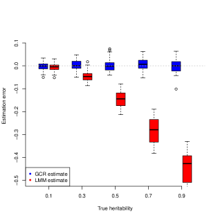
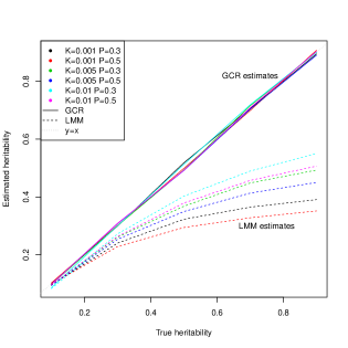
Figure 1: Comparing the performance of our GCR approach to the LMM approach of Lee et al.² on realistic simulation setups. K is the disease prevalence, P is the prevalence in the ascertained case-control study, and $h^{2}$ is the true heritability in the simulation. The left panel shows the distributions of error in estimating heritability as a function of the true heritability for a total of six simulation setups at each heritability level. We observe the significant negative bias incurred by LMM for high heritability values. The right panel shows six example scenarios, and demonstrates the increase in negative bias of LMM as both the true heritability and level of ascertainment increase. At each (heritability, P, K) combination we show the average of ten simulation repetitions.

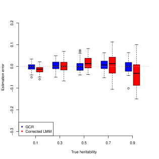
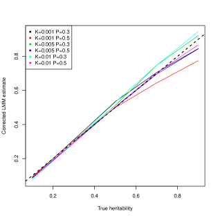
Figure 2: Heuristic correction of LMM estimates. Left - comparison of estimation errors of GCR and corrected LMM estimates, using the same simulations as in Figure 1. Right - breakdown of the average corrected estimates by K,P and $h^{2}$. We see that applying the heuristic correction yields estimates which are still much noisier than GCR estimates, but are considerably less biased than LMM estimates. The heuristic correction works best for intermediate values of the underlying heritability.

Our simulations showed that using the LMM method for heritability estimation in case-control studies yielded considerably negatively-biased estimates, while our method consistently generated unbiased estimates (Fig. 1 and Supp. Figs. 1-7).

The simulations also demonstrated a strong relation between the bias of the LMM approach and the increased variance of genetic effects due to ascertainment. This allowed us to derive a heuristic correction for the LMM heritability estimates, which corrected its bias successfully in all our simulation scenarios (Online Methods, Fig. 2 and Supp. Figs. 12-15). To validate our heuristic correction, we applied it to LMM heritability estimates for all seven WTCCC phenotypes and compared the corrected estimates to the ones obtained using GCR. The correlation between the corrected LMM estimates and GCR estimates was $0.98$, indicating that our heuristic correction generalizes beyond our particular simulations (See Online methods and Supp. material for more details).

We then applied our correction to the results of several published studies which used the LMM approach. As expected, for studies with low ascertainment or phenotypes with low heritability, the corrected estimates were not substantially different from published estimates (Alzheimer’s disease(lee2013estimation, ), endometriosis(lee2013estimation, ), schizophrenia(lee2012estimating, ) and Parkinson’s disease(do2011web, )). However, the corrected heritability estimate of multiple sclerosis – the most ascertained study we inspected – is 52.6%, compared to the uncorrected estimate of 30%. See Supp. material for more details.

An important aspect of heritability estimation is the inclusion of known (fixed) effects that should be accounted for, like known associated SNPs, known environmental effects or sex. However, estimation of fixed effects from ascertained data under the normality assumption might produce biased estimators of both the fixed effects and the heritability(burton2003correcting, ; bowden2007two, ; noh2005robust, ). Conversely, our method can be rigorously extended to allow for fixed effects (Online Methods). Our simulations suggest that GCR produces accurate estimates of heritability in the presence of fixed effects (see Supp. material for more details). Specifically for the WTCCC phenotypes, previous analysis(WTCCC, ) suggested that there’s little population structure (after removing individuals of non British descent). We validated this conclusion using the statistical test described in Patterson et al. (2006)patterson2006population (see Supp. material for more details). We therefore included only sex as a fixed effect in our heritability estimation in Table 1. The estimates of both LMM and GCR for most phenotypes without inclusion of a sex fixed effect are not substantially different from the estimates in Table 1, with the exception of the heart-disease related phenotypes (results without fixed effect not shown). For CAD in particular, it is well known that sex is a major risk factor. Accordingly, the GCR estimate without fixed effect is 71.5%, dropping to about 61% once it is added, as seen in Table 1.

GCR is computationally very efficient compared to the LMM approach (running time scales quadratically rather than cubically in the number of individuals), and so the running time is seconds rather than hours on WTCCC cohorts. As the typical size of GWAS continues to increase, this efficiency can prove critical in allowing GCR to remain computationally practical compared to other approaches. Fast running time is also useful in allowing us to use resampling approaches like the jackknife(efron1994introduction, ) for estimating confidence intervals and standard errors, rather than relying on complex and potentially inaccurate parametric approximations. All standard errors and confidence intervals we report are based on the jackknife.

We also experimented with a more involved version of our approach that included the second order term of the Taylor series expansion. This did not yield more accurate results than our first order GCR in our simulations (Supp. material).

Recently, Zuk et al.(zuk2012mystery, ) have shown an intriguing general result on the connection between the derivative of the dependence of phenotypic similarity on the proportion of identity by descent (IBD) at the average population IBD, and the narrow-sense heritability, regardless of population structure and phenotype-genotype architecture. While Zuk et al.’s result uses IBD and our method relies on estimated genetic correlations, the latter is, in fact, an unbiased estimator of the former, which is unknown. Hence, our method can produce unbiased estimators of narrow-sense heritability, even in the presence of population structure, by multiplying the estimate by a factor of (1-average population IBD).

In conclusion, our new proposed GCR method for estimation of heritability in case-control GWAS, which is based on a regression of phenotype similarities on genotype correlations, is shown to be efficient and accurate. It improves on existing methodology and generates substantially higher estimates of heritability for two major diseases inspected: Crohn’s disease and bipolar disorder. Moreover, we provide a heuristic correction for published LMM heritability estimates, which suggests that the heritability of multiple sclerosis is also considerably larger than previously thought.

Methods  
Note: An implementation of our code for GCR estimation, simulations, and heuristic correction of LMM can be accessed at: https://sites.google.com/site/davidgolanshomepage/gcr

Heritability estimation using genetic correlation regression

Liability threshold model - notations. Denote $K$ the prevalence of a condition in the population and $P$ the prevalence in the study.

Under the liability threshold model, we assume that each individual $i$ has an unknown liability $l_{i}=g_{i}+e_{i}$ where $g_{i}$ is a genetic random effect, which can be correlated across individuals, and $e_{i}$ is the environmental random effect, which is assumed to be independent of each other and of the genetic effects. Both effects are assumed to follow a Gaussian distribution with variances $\sigma_{g}^{2}$ and $1-\sigma_{g}^{2}$ respectively. A person is then assumed to be a case if her liability exceeds a threshold $t=\Phi^{-1}(1-K)$, i.e. the phenotype $y_{i}$ is given by $y_{i}=\mathbb{I}\{l_{i}>t\}$. This definition guarantees that the prevalence in the population is indeed $K.$

Selection probabilities. When the study is observational, the probability of being included in the study is independent of the phenotype. However, in a case-control study, the proportion of cases is usually greatly ascertained. To model this fact, we define a random indicator variable $s_{i}$ indicating whether individual $i$ was selected to the study.

The commonly used “full” or “complete” ascertainment assumption(stene1977assumptions, ) is $\mathbb{P}(s_{i}=1\mid y_{i}=1)=1$. While this assumption can be relaxed, as discussed later, it simplifies subsequent analysis.

Suppose the population is of size $n$ and that the expected size of the study is $n_{s}<n$. The expected number of cases in the study is $nK$. Additionally, the proportion of cases in the study is $P$, so:

$$\frac{nK}{n_{s}}=P,$$

yielding:

$$n_{s}=\frac{nK}{P}.$$

denote $p^{\prime}$ the probability of a control being included in the study (i.e. $p^{\prime}=\mathbb{P}(s_{i}=1\mid y_{i}=0)$). The expected number of controls in the study is $n(1-K)p^{\prime}$. Additionally, the proportion of controls in the study is $(1-P)$ so:

$$n(1-K)p^{\prime}=n_{s}(1-P).$$

Solving for $p^{\prime}$ yields:

$$p^{\prime}=\frac{K(1-P)}{P(1-K)}.$$

From here it follows that the probability of being included in the study for a given individual (with unknown phenotype) is:

$$K+(1-K)\frac{K(1-P)}{P(1-K)}=\frac{K}{P}.$$

Our results do not depend strictly on the full ascertainment assumption (that is, $\mathbb{P}(s_{i}=1\mid y_{i}=1)=1$). The latter assumption can be relaxed such that

$$\mathbb{P}(s_{i}=1\mid y_{i}=1)=p^{*},$$

for any $p^{*}$, as long as the probability of being selected as a control is multiplied by the same probability. This can model any step prior to the selection procedure, for example the probability that an individual is approached by the health administration to begin with. For example, a non-ascertained study ($K=P$) might involve only a proportion $p^{*}$ of the population. In this case deriving the selection probability of a given individual yields $p^{*}$ as expected.

Heritability estimation. Next, consider a pair of individuals in the study, whose genetic effects are correlated and denote by $\rho$ the correlation between their genetic effects.

Denote by $Z_{ij}$ the product of the standardized phenotypes:

$$Z_{ij}=\frac{(y_{i}-P)(y_{j}-P)}{P(1-P)}.$$

The variable $Z_{ij}$ can take three values:

$$Z_{ij}=\begin{cases}\frac{1-P}{P}\;\;\;\;&y_{i}=y_{j}=1\\ -1&y_{i}\neq y_{j}\\ \frac{P}{1-P}&y_{i}=y_{j}=0\end{cases}.$$

We write down the expected value of $Z_{ij}$, conditional on the fact that $s_{i}=s_{j}=1$ (the individuals are part of the study) and given $\rho$:

$$\mathbb{E}[Z_{ij}\mid s_{i}=s_{j}=1;\rho] = \frac{1-P}{P}\mathbb{P}(y_{i}=y_{j}=1\mid s_{i}=s_{j}=1;\rho)-$$

$$\mathbb{P}(y_{i}\neq y_{j}\mid s_{i}=s_{j}=1;\rho)+\frac{P}{1-P}\mathbb{P}(y_{i}=y_{j}=0\mid s_{i}=s_{j}=1;\rho).$$

We apply Bayes rule to the first of the three expressions on the right:

$$\mathbb{P}(y_{i}=y_{j}=1\mid s_{i}=s_{j}=1;\rho)=\frac{\mathbb{P}(s_{i}=s_{j}=1\mid y_{i}=y_{j}=1;\rho)\mathbb{P}(y_{i}=y_{j}=1;\rho)}{\mathbb{P}(s_{i}=s_{j}=1;\rho)}.$$

Under the full ascertainment assumption $\mathbb{P}(s_{i}=s_{j}=1\mid y_{i}=y_{j}=1;\rho)=1$, and so

$$\mathbb{P}(y_{i}=y_{j}=1\mid s_{i}=s_{j}=1;\rho)=\frac{\mathbb{P}(y_{i}=y_{j}=1;\rho)}{\mathbb{P}(s_{i}=s_{j}=1;\rho)}.$$

Similarly:

$$\mathbb{P}(y_{i}=y_{j}=0\mid s_{i}=s_{j}=1;\rho)=\frac{\mathbb{P}(s_{i}=s_{j}=1\mid y_{i}=y_{j}=0;\rho)\mathbb{P}(y_{i}=y_{j}=0;\rho)}{\mathbb{P}(s_{i}=s_{j}=1;\rho)},$$

and since a control is selected to the study with probability $\frac{K(1-P)}{P(1-K)}$, this boils down to:

$$\Big{(}\frac{K(1-P)}{P(1-K)}\Big{)}^{2}\frac{\mathbb{P}(y_{i}=y_{j}=0;\rho)}{\mathbb{P}(s_{i}=s_{j}=1;\rho)}.$$

For the case of $y_{i}\neq y_{j}$, one individual is a case, and is automatically selected, while the other is a control and is selected with probability $\frac{K(1-P)}{P(1-K)}$. Hence:

$$\mathbb{P}(y_{i}\neq y_{j}\mid s_{i}=s_{j}=1;\rho)=\frac{K(1-P)}{P(1-K)}\frac{\mathbb{P}(y_{i}\neq y_{j};\rho)}{\mathbb{P}(s_{i}=s_{j}=1;\rho)},$$

Using these results we get:

$$\mathbb{E}[Z_{ij}\mid s_{i}=s_{j}=1;\rho]=$$

$$\frac{\frac{1-P}{P}\mathbb{P}(y_{i}=y_{j}=1;\rho)-\frac{K(1-P)}{P(1-K)}\mathbb{P}(y_{i}\neq y_{j};\rho)+\frac{P}{1-P}\Big{(}\frac{K(1-P)}{P(1-K)}\Big{)}^{2}\mathbb{P}(y_{i}=y_{j}=0;\rho)}{\mathbb{P}(s_{i}=s_{j}=1;\rho)}.$$

Denote the numerator by $A(\rho)$ and the denominator by $B(\rho)$. We wish to approximate the last equation using a Taylor series around $\rho=0$. Since the individuals are unrelated, the correlation is expected to be close to 0, and therefore such an approximation is expected to be good. Such an approximation would take the form:

$$\mathbb{E}[Z_{ij}\mid s_{i}=s_{j}=1;\rho]\approx\frac{A(0)}{B(0)}+\frac{A^{\prime}(0)B(0)+B^{\prime}(0)A(0)}{B(0)^{2}}\rho.$$

See Supp. Mat. for a discussion of a second order approximation.

Note that with $\rho=0$, the phenotypes of the two individuals are i.i.d. and so $A(0)=0$. Therefore, the Taylor approximation can be simplified:

$$\mathbb{E}[Z_{ij}\mid s_{i}=s_{j}=1;\rho]\approx\frac{A^{\prime}(0)}{B(0)}\rho.$$

Similarly, with $\rho=0$ the events of being included in the study are i.i.d. for both individuals, so $B(0)=\frac{K^{2}}{P^{2}}$.

All that remains is to find $A^{\prime}(0)$. Towards that end, we are interested in computing the probabilities of the three possible combinations of phenotypes:

$$\mathbb{P}(y_{i}=y_{j}=1;\rho,\sigma_{g}^{2})=\int_{t}^{\infty}\int_{t}^{\infty}f_{\rho,\sigma_{g}^{2}}(l_{1},l_{2})dl_{1}dl_{2},$$

$$\mathbb{P}(y_{i}\neq y_{j};\rho,\sigma_{g}^{2})=2\int_{-\infty}^{t}\int_{t}^{\infty}f_{\rho,\sigma_{g}^{2}}(l_{1},l_{2})dl_{1}dl_{2},$$

and

$$\mathbb{P}(y_{i}=y_{j}=0;\rho,\sigma_{g}^{2})=\int_{-\infty}^{t}\int_{-\infty}^{t}f_{\rho,\sigma_{g}^{2}}(l_{1},l_{2})dl_{1}dl_{2},$$

where $f_{\rho,\sigma_{g}^{2}}$ is the multivariate Gaussian density, namely:

$$f_{\rho,\sigma_{g}^{2}}(l_{1},l_{2})=\frac{1}{2\pi}|\Sigma|^{-\frac{1}{2}}e^{-\frac{(l_{1},l_{2})\Sigma^{-1}(l_{1},l_{2})^{\intercal}}{2}},$$

with $\Sigma$ denoting the covariance matrix of the liabilities, given explicitly by:

$$\Sigma=\left(\begin{array}[]{cc}1&\rho\\ \rho&1\end{array}\right)\sigma_{g}^{2}+\left(\begin{array}[]{cc}1&0\\ 0&1\end{array}\right)(1-\sigma_{g}^{2})=\left(\begin{array}[]{cc}1&\rho\sigma_{g}^{2}\\ \rho\sigma_{g}^{2}&1\end{array}\right).$$

The determinant of $\Sigma$ is $|\Sigma|=1-\rho^{2}\sigma_{g}^{4}$ and its inverse is $\Sigma^{-1}=\frac{1}{1-\rho^{2}\sigma_{g}^{4}}\left(\begin{array}[]{cc}1&-\rho\sigma_{g}^{2}\\ -\rho\sigma_{g}^{2}&1\end{array}\right),$ and so the density function $f_{\rho,\sigma_{g}^{2}}$ can be written as:

$$f_{\rho,\sigma_{g}^{2}}(l_{1},l_{2})=\frac{1}{2\pi\sqrt{1-\rho^{2}\sigma_{g}^{4}}}e^{-\frac{l_{1}^{2}+l_{2}^{2}-2l_{1}l_{2}\rho\sigma_{g}^{2}}{2(1-\rho^{2}\sigma_{g}^{4})}}.$$

Differentiating $A(\rho)$ requires differentiating each of the three double integrals w.r.t. $\rho$:

$$\frac{d}{d\rho}\int_{t}^{\infty}\int_{t}^{\infty}f_{\rho,\sigma_{g}^{2}}(l_{1},l_{2})dl_{1}dl_{2}=\int_{t}^{\infty}\int_{t}^{\infty}\frac{d}{d\rho}f_{\rho,\sigma_{g}^{2}}(l_{1},l_{2})dl_{1}dl_{2}.$$

Setting $\rho=0$ in the last expression yields:

$$\int_{t}^{\infty}\int_{t}^{\infty}l_{1}l_{2}\sigma_{g}^{2}\frac{1}{2\pi}e^{-\frac{l_{1}^{2}+l_{2}^{2}}{2}}=\sigma_{g}^{2}\Big{[}\int_{t}^{\infty}l\frac{1}{\sqrt{2\pi}}e^{-\frac{l^{2}}{2}}dl\Big{]}^{2}=\sigma_{g}^{2}\varphi(t)^{2}.$$

Explanation: we differentiate and set $\rho=0$. By the chain rule, the derivative of any expression with $\rho^{2}$ is $0$ at $\rho=0$, and obviously the derivative of any expression which does not depend on $\rho$ is $0$. The only expression whose derivative is therefore not $0$ at $\rho=0$ is $-2l_{1}l_{2}\rho\sigma_{g}^{2}$ in the numerator of the exponent. The denominator of the exponent is $2$ at $\rho=0$, and so the derivative at $\rho=0$ is $l_{1}l_{2}\sigma_{g}^{2}\frac{1}{2\pi}e^{-\frac{l_{1}^{2}+l_{2}^{2}}{2}}$. Similarly:

$$\frac{d}{d\rho}\int_{-\infty}^{t}\int_{t}^{\infty}f_{\rho,\sigma_{g}^{2}}(l_{1},l_{2})dl_{1}dl_{2}=-\sigma_{g}^{2}\varphi(t)^{2},$$

and

$$\frac{d}{d\rho}\int_{-\infty}^{t}\int_{-\infty}^{t}\,f_{\rho,\sigma_{g}^{2}}(l_{1},l_{2})dl_{1}dl_{2}=\sigma_{g}^{2}\varphi(t)^{2}.$$

Using these results we can write down $A^{\prime}(0)$:

$$A^{\prime}(0)=\Big{[}\frac{1-P}{P}+2\frac{K(1-P)}{P(1-K)}+\frac{P}{1-P}\Big{(}\frac{K(1-P)}{P(1-K)}\Big{)}^{2}\Big{]}\sigma_{g}^{2}\varphi(t)^{2}=\frac{1-P}{P(1-K)^{2}}\sigma_{g}^{2}\varphi(t)^{2},$$

and so:

$$\mathbb{E}[Z_{ij}\mid s_{i}=s_{j}=1;\rho]\approx\frac{A^{\prime}(0)}{B(0)}\rho=\frac{\frac{1-P}{P(1-K)^{2}}\sigma_{g}^{2}\varphi(t)^{2}}{\frac{K^{2}}{P^{2}}}\rho=\frac{P(1-P)}{K^{2}(1-K)^{2}}\sigma_{g}^{2}\varphi(t)^{2}\rho.$$

Hence, when the error of the approximation is small, the slope obtained by regressing $Z_{ij}$ on $G_{ij}$ is an unbiased estimator of $\frac{P(1-P)}{K^{2}(1-K)^{2}}\sigma_{g}^{2}\varphi(t)^{2}$, thus dividing it by $\frac{P(1-P)}{K^{2}(1-K)^{2}}\varphi(t)^{2}$ yields an unbiased estimator of $\sigma_{g}^{2}$ - the liability scale heritability.

Extending the liability threshold model to include fixed effects. It is often desired to include fixed effects in the analysis of a complex phenotype. Such fixed effects might include external information such as sex, diet and exposure to environmental risks, but can also be genetic variants with known effects or estimates of population structure such as projections of several top principal components.

Since the liability threshold model is in fact a probit model, fixed effects can be included in the usual manner:

$$l_{i}=x_{i}^{\intercal}\beta+g_{i}+e_{i},$$

where $x_{i}$ is a vector of the values of the relevant covariates and $\beta$ is a vector of their respective effect sizes.

An individual is a case if $l_{i}>t$, as before. However, an equivalent formulation would be to subtract the fixed effect from the threshold, rather than adding it to the liability:

$$t_{i}=t-x_{i}^{\intercal}\beta,$$

thus keeping the previous formulation of the liability as a sum of genetic and environmental effects.

Heritability estimation with known fixed effects. Assume first that the fixed effects are known, and so the $t_{i}$’s are known. The probability of being a case, and of being included in the study, are no longer equal for all the observed individuals. We denote:

$$K_{i}=\mathbb{P}(y_{i}=1;t_{i}),$$

the probability that the $i$’th individual is a case, and:

$$P_{i}=\mathbb{P}(y_{i}=1\mid s_{i}=1;t_{i}),$$

the probability that the $i$’th individual is a case conditional on being selected for the study, where $t_{i}$ is computed using the fixed effects as described above. We now wish to derive the same first order approximation, while accounting for the newly introduced heterogeneity. We redefine:

$$Z_{ij}=\frac{(y_{i}-P_{i})(y_{j}-P_{j})}{\sqrt{P_{i}(1-P_{i})}\sqrt{P_{j}(1-P_{j})}},$$

and follow the same steps as before (see supplementary materials for a full derivation). Using the first order Taylor approximation we conclude that the slope obtained by regressing $Z_{ij}$ on

$$\frac{\varphi(t_{i})\varphi(t_{j})\Big{[}1-(P_{i}+P_{j})\Big{(}\frac{P-K}{P(1-K)}\Big{)}+P_{i}P_{j}\Big{(}\frac{P-K}{P(1-K)}\Big{)}^{2}\Big{]}}{\sqrt{P_{i}(1-P_{i})}\sqrt{P_{j}(1-P_{j})}\Big{(}K_{i}+(1-K_{i})\frac{K(1-P)}{P(1-K)}\Big{)}\Big{(}K_{j}+(1-K_{j})\frac{K(1-P)}{P(1-K)}\Big{)}}G_{ij},$$

is an estimator of heritability on the liability scale.

Estimating heritability with unknown fixed effects. More often than not, the effects of relevant fixed effects are unknown and must be estimated from the data. However, estimating effect sizes under ascertainment in case-control studies is notoriously problematic. Specifically, under the threshold (probit) model, ignoring the ascertainment yields biased estimators.

A special exception is the case of logistic regression. In their seminal paper, Prentice and Pyke (1979)(prentice1979logistic, ) proved that using a logistic regression to estimate fixed effects from ascertained data yields consistent estimators of these effects in the (unascertained) population, and that the ascertainment only biases the intercept.

We therefore suggest a two-step procedure for estimating heritability. First, we estimate the fixed effects using a logistic regression model. We then correct the effect of the ascertainment, and obtain the individual-specific thresholds. Lastly, we plug the thresholds into the estimation scheme described above.

More elaborately, by Bayes’ formula:

$$P_{i}=\frac{\mathbb{P}(s_{i}=1\mid y_{i}=1;x_{i})K_{i}}{\mathbb{P}(s_{i}=1;x_{i})},$$

by the complete ascertainment assumption $\mathbb{P}(s_{i}=1\mid y_{i}=1,x_{i})=1$, and according to the selection scheme:

$$\mathbb{P}(s_{i}=1;x_{i})=K_{i}+\frac{K(1-P)}{P(1-K)}\big{(}1-K_{i}\big{)}.$$

We can thus solve for $K_{i}$ and express it is a function of $P_{i}$:

$$K_{i}=\frac{\frac{K(1-P)}{P(1-K)}P_{i}}{1+\frac{K(1-P)}{P(1-K)}P_{i}-P_{i}}$$

We then use logistic regression to obtain $\hat{P}_{i}$ - a consistent estimator of $P_{i}$, and use this estimate to obtain an estimate of $K_{i}$, which is in turn used to estimate the threshold:

$$\hat{t}_{i}=\Phi^{-1}\big{(}1-\hat{K}_{i}\big{)},$$

and the estimates of the individual-wise thresholds are used for estimating the variance of the genetic effect.

Estimating the added variance due to fixed effects Lastly, the presence of fixed effects increases the variance of the liability, so $\sigma_{g}^{2}$ no longer equals $h^{2}$. The appropriate definition of heritability is now:

$$h^{2}=\frac{\sigma_{g}^{2}}{\sigma_{g}^{2}+\sigma_{e}^{2}+\sigma_{t}^{2}}=\frac{\sigma_{g}^{2}}{1+\sigma_{t}^{2}},$$

where $\sigma_{t}^{2}$ is the variance of the thresholds in the population, and so the estimate of $\sigma_{g}^{2}$ can be transformed to an estimate of the heritability simply by dividing it by $1+\sigma_{t}^{2}$. We discuss how $\sigma_{t}^{2}$ can be estimated from the data in the Supplementary material.

Simulations using a generative model

Our goal was to create a realistic simulation, covering a wide range of combinations of disease prevalence $K$, case sampling probability $P$ and heritability $\sigma^{2}_{g}$, and for each one creating “natural” genotypes that realistically recreate the complex correlation structure induced by case-control sampling.

Given these parameters, our simulations proceeded as follows:

1. The MAFs of 10,000 SNPs were randomly sampled from $U[0.05,0.5]$.

2. SNP effect sizes were randomly sampled from $N(0,\frac{\sigma_{g}^{2}}{m}).$

3. For each individual, we:

   1. Randomly generated a genotype using the MAFs, and normalized it (according to Yang et al.’s model(yang2011gcta, )).

   2. Used the genotype and the effect sizes, to compute the genetic effect.

   3. Sampled an environmental effect from $N(0,1-\sigma_{g}^{2})$.

   4. Computed liability and phenotype.

   5. If the phenotype was a case - the individual was automatically included in the study. Otherwise the individual was included in the study with probability $\frac{K(1-P)}{P(1-K)}$.

4. Step (2) was repeated until enough individuals were accumulated (4,000).

5. The genotypes of all included individuals were used to compute $G=\frac{ZZ^{\intercal}}{m}$ where $Z$ is the matrix of n5.8alized genotypes.

This matrix $G$ was then used to estimate heritability for the LMM using the $GCTA$ software(yang2011gcta, ) and the correction of Lee et al.(Lee2011estimating, ); and using GCR as described above.

We note that our choice to work with SNPs that are in linkage equilibrium was motivated by the analysis of Patterson et al.patterson2006population . They show that for the purpose of generating correlation matrices, using SNPs in linkage disequilibrium (LD) is equivalent to using a smaller number of SNPs in linkage equilibrium. They also suggest a method for estimating the effective number of SNPs (i.e. the number of SNPs in linkage equilibrium leading to the same distribution of correlation matrices as a given set of SNPs in LD). Applying their method to WTCCC data suggests that the effective number of SNPs in linkage equilibrium is roughly one tenth of the actual number of SNPs. Hence, using 10,000 SNPs in our simulations is equivalent to simulating roughly 100,000 SNPs with realistic LD structure.

Heuristic correction for the LMM approach

Denote the estimate of the heritability on the liability scale, obtained through the method of Lee et al.(Lee2011estimating, ) by $\tilde{\sigma}^{2}_{g}$, and the estimates obtained by our method by $\hat{\sigma}^{2}_{g}$. Denote the true variance of the genetic effect under ascertainment by:

$$\sigma_{g_{cc}}^{2}=\sigma_{g}^{2}\Big{[}1+\sigma_{g}^{2}\varphi(t)\frac{(P-K)}{K(1-K)}\Big{[}t-\varphi(t)\frac{(P-K)}{K(1-K)}\Big{]}\Big{]}.$$

We note a different analytical expression of $\sigma_{g_{cc}}^{2}$ is given in(Lee2011estimating, ). We validated correctness of our derivation of this expression numerically.

As detailed in the Supplementary Materials, our simulations demonstrated the following properties of these estimators:

1. They are both unbiased when there is no ascertainment.

2. Our estimate $\hat{\sigma}^{2}_{g}$ remains unbiased in all situations. However, in presence of ascertainment, $\tilde{\sigma}^{2}_{g}$ is biased, and is not linear in the true $\sigma^{2}_{g}$ for fixed $K,P$.

3. When multiplied by $\sigma_{g_{cc}}^{2}/\sigma_{g}^{2}$, the estimate $\tilde{\sigma}^{2}_{g}$ becomes linear in $\sigma^{2}_{g}$ for fixed $K,P$.

4. The bias of $\tilde{\sigma}^{2}_{g}$ worsens as the ascertainment factor $\frac{K}{P}$ decreases.

We therefore performed an extensive analysis of the relationship between $\frac{K}{P}$ and the bias of the “linearized” estimate $\tilde{\sigma}^{2}_{g}\frac{\sigma_{g_{cc}}^{2}}{\sigma_{g}^{2}}$ in our simulations. Our analysis, as detailed in Supplementary Materials, led us to the following relationship between $\tilde{\sigma}^{2}_{g}$ and the true underlying heritability $\sigma_{g}^{2}$:

$$\mathbb{E}\tilde{\sigma}^{*2}_{g}\approx\frac{K^{2}(1-K)^{2}}{\varphi(t)^{2}P(1-P)}(1.3-0.3\sqrt{\frac{K}{P}})\frac{\sigma_{g}^{4}}{\sigma_{g_{cc}}^{2}}.$$

Correcting published results We have derived our heuristic correction using simulations wherein the true underlying heritability is known. However, contrary to previously used corrections, our correction is not a linear transformation of the estimate. When attempting to correct published estimates, we only know $K,P$ and $\tilde{\sigma}_{g}^{2}$. We define our corrected estimate $\hat{\sigma}_{g}^{*2}$ to be the value of $\sigma_{g}^{2}$ for which

$$\mathbb{E}[\tilde{\sigma}_{g}^{2};\sigma_{g}^{2}=\hat{\sigma}_{g}^{*2}]=\tilde{\sigma}_{g}^{2},$$

where the expectation is computed using the approximate relationship we derived previously. In other words, the corrected estimate of heritability is the value of heritability for which the expectation of the estimator is the observed estimate, where the expectation is calculated using our heuristic correction.

Confidence intervals are derived by applying the same procedure to the top and bottom limits of a $95\%$ confidence interval based on the published standard deviation of the estimate.

Phenotype	Prevalence (%)	LMM (sd) (%)	GCR (sd) (%)	Family studies (%)
CD	0.1	23.2 (3)	34.1 (5.8)	50-60
BD	0.5	42.8 (4.1)	53.8 (6.8)	71
T2D	3	42 (6.3)	47.8 (9.9)	26-69
HT	5	53.1 (7.4)	52.3 (10.6)	31-63**
CAD	30	66.9 (12.8)	61.1 (16.9)	39-56**
RA	0.75	16.5 (4.6)	17.9 (7)	53-65
T1D*	0.5	16.1 (4.2)	17.2 (5.8)	72-88

Table 1: Comparing estimated heritability of 7 WTCCC studies using GCR, LMM and family-based estimates. Standard deviations are given in parentheses. GCR and LMM estimates are adjusted for imperfect LD as discussed in ¹, and include sex as a fixed effect. GCR standard deviations are estimated using 1,000 jackknife iterations and LMM standard deviations are produced by the GCTA software²⁷. Population prevalence and family-based estimates are from ², ²⁸, ¹³, ²⁹, ³⁰, ³¹, ³², ³³, ³⁴, ³⁵, ¹⁸, ³⁶, ³⁷.
$*$ Analysis does not include chromosome 6.
$**$ Estimates might not be comparable to GCR/LMM estimates due to different phenotype definitions.

References

- 1 Yang, J., Benyamin, B., McEvoy, B. P., Gordon, S., Henders, A. K., Nyholt, D. R., Madden, P. A., Heath, A. C., Martin, N. G., Montgomery, G. W., et al. Common snps explain a large proportion of the heritability for human height. Nature genetics 42(7), 565–569 (2010).
- 2 Lee, S. H., Wray, N. R., Goddard, M. E., and Visscher, P. M. Estimating missing heritability for disease from genome-wide association studies. The American Journal of Human Genetics 88(3), 294–305 (2011).
- 3 Do, C. B., Tung, J. Y., Dorfman, E., Kiefer, A. K., Drabant, E. M., Francke, U., Mountain, J. L., Goldman, S. M., Tanner, C. M., Langston, J. W., et al. Web-based genome-wide association study identifies two novel loci and a substantial genetic component for parkinson’s disease. PLoS genetics 7(6), e1002141 (2011).
- 4 Lee, S. H., DeCandia, T. R., Ripke, S., Yang, J., Sullivan, P. F., Goddard, M. E., Keller, M. C., Visscher, P. M., Wray, N. R., et al. Estimating the proportion of variation in susceptibility to schizophrenia captured by common snps. Nature genetics 44(3), 247–250 (2012).
- 5 Lee, S. H., Harold, D., Nyholt, D. R., Goddard, M. E., Zondervan, K. T., Williams, J., Montgomery, G. W., Wray, N. R., and Visscher, P. M. Estimation and partitioning of polygenic variation captured by common snps for alzheimer’s disease, multiple sclerosis and endometriosis. Human molecular genetics 22(4), 832–841 (2013).
- 6 Bloom, J. S., Ehrenreich, I. M., Loo, W., Lite, T.-L. V., and Kruglyak, L. Finding the sources of missing heritability in a yeast cross. arXiv preprint arXiv:1208.2865 (2012).
- 7 Eichler, E. E., Flint, J., Gibson, G., Kong, A., Leal, S. M., Moore, J. H., and Nadeau, J. H. Missing heritability and strategies for finding the underlying causes of complex disease. Nature Reviews Genetics 11(6), 446–450 (2010).
- 8 Maher, B. The case of the missing heritability. Nature 456(7218), 18–21 (2008).
- 9 Manolio, T. A., Collins, F. S., Cox, N. J., Goldstein, D. B., Hindorff, L. A., Hunter, D. J., McCarthy, M. I., Ramos, E. M., Cardon, L. R., Chakravarti, A., et al. Finding the missing heritability of complex diseases. Nature 461(7265), 747–753 (2009).
- 10 Zuk, O., Hechter, E., Sunyaev, S. R., and Lander, E. S. The mystery of missing heritability: Genetic interactions create phantom heritability. Proceedings of the National Academy of Sciences 109(4), 1193–1198 (2012).
- 11 Nielsen, R., Paul, J. S., Albrechtsen, A., and Song, Y. S. Genotype and snp calling from next-generation sequencing data. Nature Reviews Genetics 12(6), 443–451 (2011).
- 12 Visscher, P. M. Sizing up human height variation. Nature genetics 40(5), 489–490 (2008).
- 13 Dudbridge, F. Power and predictive accuracy of polygenic risk scores. PLoS Genetics 9(3), e1003348 (2013).
- 14 Yang, J., Manolio, T. A., Pasquale, L. R., Boerwinkle, E., Caporaso, N., Cunningham, J. M., de Andrade, M., Feenstra, B., Feingold, E., Hayes, M. G., et al. Genome partitioning of genetic variation for complex traits using common snps. Nature genetics 43(6), 519–525 (2011).
- 15 Price, A. L., Helgason, A., Thorleifsson, G., McCarroll, S. A., Kong, A., and Stefansson, K. Single-tissue and cross-tissue heritability of gene expression via identity-by-descent in related or unrelated individuals. PLoS Genetics 7(2), e1001317 (2011).
- 16 Visscher, P. M., Hill, W. G., and Wray, N. R. Heritability in the genomics era—concepts and misconceptions. Nature Reviews Genetics 9(4), 255–266 (2008).
- 17 Dempster, E. R. and Lerner, I. M. Heritability of threshold characters. Genetics 35(2), 212 (1950).
- 18 Burton, P. R., Clayton, D. G., Cardon, L. R., Craddock, N., Deloukas, P., Duncanson, A., Kwiatkowski, D. P., McCarthy, M. I., Ouwehand, W. H., Samani, N. J., et al. Genome-wide association study of 14,000 cases of seven common diseases and 3,000 shared controls. Nature 447(7145), 661–678 (2007).
- 19 Zhou, X., Carbonetto, P., and Stephens, M. Polygenic modeling with bayesian sparse linear mixed models. PLoS Genetics 9(2), e1003264 (2013).
- 20 Burton, P. R. Correcting for nonrandom ascertainment in generalized linear mixed models (glmms), fitted using gibbs sampling. Genetic epidemiology 24(1), 24–35 (2003).
- 21 Bowden, J., Thompson, J., and Burton, P. A two-stage approach to the correction of ascertainment bias in complex genetic studies involving variance components. Annals of Human Genetics 71(2), 220–229 (2007).
- 22 Noh, M., Lee, Y., and Pawitan, Y. Robust ascertainment-adjusted parameter estimation. Genetic epidemiology 29(1), 68–75 (2005).
- 23 Patterson, N., Price, A. L., and Reich, D. Population structure and eigenanalysis. PLoS genetics 2(12), e190 (2006).
- 24 Efron, B. and Tibshirani, R. J. An introduction to the bootstrap (chapman & hall/crc monographs on statistics & applied probability). (1994).
- 25 Stene, J. Assumptions for different ascertainment models in human genetics. Biometrics , 523–527 (1977).
- 26 Prentice, R. L. and Pyke, R. Logistic disease incidence models and case-control studies. Biometrika 66(3), 403–411 (1979).
- 27 Yang, J., Lee, S. H., Goddard, M. E., and Visscher, P. M. Gcta: a tool for genome-wide complex trait analysis. American journal of human genetics 88(1), 76 (2011).
- 28 Wray, N. R., Yang, J., Goddard, M. E., and Visscher, P. M. The genetic interpretation of area under the roc curve in genomic profiling. PLoS genetics 6(2), e1000864 (2010).
- 29 Almgren, P., Lehtovirta, M., Isomaa, B., Sarelin, L., Taskinen, M., Lyssenko, V., Tuomi, T., and Groop, L. Heritability and familiality of type 2 diabetes and related quantitative traits in the botnia study. Diabetologia 54(11), 2811–2819 (2011).
- 30 Poulsen, P., Kyvik, K. O., Vaag, A., and Beck-Nielsen, H. Heritability of type ii (non-insulin-dependent) diabetes mellitus and abnormal glucose tolerance–a population-based twin study. Diabetologia 42(2), 139–145 (1999).
- 31 Sofaer, J. Crohn’s disease: the genetic contribution. Gut 34(7), 869–871 (1993).
- 32 Edvardsen, J., Torgersen, S., Røysamb, E., Lygren, S., Skre, I., Onstad, S., and Øien, P. A. Heritability of bipolar spectrum disorders. unity or heterogeneity? Journal of affective disorders (2008).
- 33 Kyvik, K. O., Green, A., and Beck-Nielsen, H. Concordance rates of insulin dependent diabetes mellitus: a population based study of young danish twins. BMJ 311(7010), 913–917 (1995).
- 34 Hyttinen, V., Kaprio, J., Kinnunen, L., Koskenvuo, M., and Tuomilehto, J. Genetic liability of type 1 diabetes and the onset age among 22,650 young finnish twin pairs a nationwide follow-up study. Diabetes 52(4), 1052–1055 (2003).
- 35 23andme. 23andme website, (2013). [https://www.23andme.com/. Online; accessed 20-April-2013].
- 36 British Heart Foundation. BHF website, (2013). [http://www.bhf.org.uk/publications/view-publication.aspx?ps=1002097. Online; accessed 8-May-2013].
- 37 Kupper, N., Willemsen, G., Riese, H., Posthuma, D., Boomsma, D. I., and de Geus, E. J. Heritability of daytime ambulatory blood pressure in an extended twin design. Hypertension 45(1), 80–85 (2005).