Harmonically trapped Fermi gas: Temperature dependence of the Tan contact

Abstract

Ultracold atomic gases with short-range interactions are characterized by a number of universal species-independent relations. Many of these relations involve the two-body Tan contact. Employing the canonical ensemble, we determine the Tan contact for small harmonically trapped two-component Fermi gases at unitarity over a wide range of temperatures, including the zero and high temperature regimes. A cluster expansion that describes the properties of the $N$-particle system in terms of those of smaller subsystems is introduced and shown to provide an accurate description of the contact in the high temperature regime. Finite-range corrections are quantified and the role of the Fermi statistics is elucidated by comparing results for Fermi, Bose and Boltzmann statistics.

Systems with short-range interactions are characterized by universal relations that are independent of the details of the underlying interactions. The Tan contact Tan1 ; Tan2 ; Tan3 ; castin ; braaten , e.g., enters into a large number of universal relations and connects physically distinct quantities such as the large momentum tail, the inelastic loss rate, the number of pairs with small interparticle distances, and certain characteristics of radio frequency (rf) spectra. A striking feature of many of the universal relations is that they apply to homogeneous and inhomogeneous systems at zero and finite temperature.

Yet, although many universal relations that evolve around the Tan contact are known, only a few explicit measurements earlyJin ; Vale2010 ; Vale2011 ; Jin12 ; hoinka and calculations DailyBlume ; werner09 ; strinati ; drut ; svistunov ; boettcher ; zwerger ; doggen of the Tan contact exist. At present, the dependence of the Tan contact of the spin-balanced homogeneous two-component Fermi gas at unitarity on the temperature is highly debated. While experimental data Jin12 , extracted from the rf lineshape of a potassium mixture in two different hyperfine states, indicate a fairly sharp jump of the contact around the superfluid transition temperature, two sets of Monte Carlo simulations drut ; svistunov —which disagree with each other—do not seem to see this jump.

This paper considers small Fermi gases consisting of $N_{1}$ spin-up and $N_{2}$ spin-down fermions under external spherically symmetric harmonic confinement. Working in the canonical ensemble, we determine the Tan contact at unitarity with an accuracy at the few percent level as a function of the temperature, including the low (near zero) temperature regime and the high temperature regime. Our main findings are: (i) The high temperature tail of the contact $C_{N_{1},N_{2}}$ is well approximated by the contacts of the $(N_{1}^{\prime},N_{2}^{\prime})$ subclusters with $N_{1}^{\prime}+N_{2}^{\prime}<N$, where $N_{1}^{\prime}\leq N_{1}$ and $N_{2}^{\prime}\leq N_{2}$. The connection between this cluster expansion, which can be applied to any thermodynamic observable calculated in the canonical ensemble, and the virial expansion that has recently been applied extensively to determine thermodynamic properties of atomic gases in the grand canonical ensemble JasonHo ; Drummond ; liurev , is described. (ii) While the contact of the trapped $(N_{1},N_{2})=(1,1)$ and $(2,2)$ systems is maximal at $T=0$, that of the $(2,1)$, $(3,1)$ and $(4,1)$ systems shows a maximum at finite temperature. A microscopic interpretation of this behavior is offered. (iii) For the cases studied, the contact shows a non-negligible dependence on the range $r_{0}$ of the underlying two-body potential at low temperature; in the high temperature regime, in contrast, the range dependence is negligible. (iv) Fermi statistics plays a role at temperatures where three-body physics is non-negligible. The role of the Fermi statistics is elucidated by turning the exchange symmetry off and by switching to Bose statistics.

The two-component Fermi gas consisting of $N$ atoms with mass $m$ and position vectors $\mathbf{r}_{j}$ ($j=1,\cdots,N$) is described by the model Hamiltonian $H$,

$$H=\sum_{j=1}^{N}\left(\frac{-\hbar^{2}}{2m}\nabla_{j}^{2}+\frac{1}{2}m\omega^{2}\mathbf{r}_{j}^{2}\right)+\sum_{j=1}^{N_{1}}\sum_{k=N_{1}+1}^{N}V_{\text{tb}}(\mathbf{r}_{jk}),$$ (1)

where $\omega$ denotes the angular trapping frequency. We consider two different interspecies two-body potentials $V_{\text{tb}}$, a regularized zero-range pseudopotential $V_{\text{F}}$ Yang1957 and a short-range Gaussian potential $V_{\text{G}}$ with depth $U_{0}$ ($U_{0}<0$) and range $r_{0}$, $V_{\text{G}}(\mathbf{r}_{jk})=U_{0}\exp[-\mathbf{r}_{jk}^{2}/(2r_{0}^{2})]$. For a given $r_{0}$, we adjust $U_{0}$ such that $V_{\text{G}}$ supports a single zero-energy $s$-wave bound state in free space, i.e., such that the $s$-wave scattering length $a_{s}$ diverges. Our calculations use $r_{0}\ll a_{\text{ho}}$, where $a_{\text{ho}}$ is the harmonic oscillator length, $a_{\text{ho}}=\sqrt{\hbar/(m\omega)}$. This Letter considers temperatures ranging from $T=0$ to $k_{B}T\gg E_{\text{ho}}$, where $E_{\text{ho}}=\hbar\omega$. The largest temperatures considered are chosen such that the two-body interactions can be reliably parametrized by the $s$-wave scattering length and corresponding effective range correction, i.e., so that higher partial wave contributions in the two-body sector can be neglected.

To determine the Tan contact $C_{N_{1},N_{2}}$, we employ the adiabatic and pair relations,

$$C_{N_{1},N_{2}}=\frac{4\pi m}{\hbar^{2}}\left\langle\frac{\partial E(a_{s})}{\partial(-a_{s}^{-1})}\right\rangle_{\text{th}}$$ (2)

and

$$C_{N_{1},N_{2}}=4\pi\lim_{s\to 0}\frac{\langle N_{\text{pair}}^{r<s}\rangle_{\text{th}}}{s};$$ (3)

here, the $\langle\cdot\rangle_{\text{th}}$ notation indicates a thermal average and $E(a_{s})$ denotes the energy of the system. The quantity $N_{\text{pair}}^{r<s}$ is the number of pairs with interspecies distances smaller than $s$. For zero-range interactions, $s$ is taken to zero. For finite-range interactions, in contrast, $s$ goes to a small value such that $s$ is larger than the range $r_{0}$ of the underlying two-body potential. The pair relation can be written in terms of the short distance behavior of the pair distribution function $P_{12}(r)$ for the spin-up—spin-down pairs Tan1 ; Tan2 ; Tan3 ; DailyBlume . Throughout, we employ the normalization $4\pi\int_{0}^{\infty}P_{12}(r)r^{2}dr=N_{1}N_{2}$. The thermally averaged expectation values are obtained by employing two complementary approaches, a “microscopic approach” and a “direct approach”.

In the microscopic approach, the thermal expectation value of an observable $A$ is obtained using $\langle A\rangle_{\text{th}}=\sum_{j}\exp[-E_{j}/(k_{B}T)]A_{j}/\sum_{j}\exp[-E_{j}/(k_{B}T)]$, where the sum runs over all eigen energies $E_{j}$ (with associated eigen states $\psi_{j}$) of the Hamiltonian $H$ and $A_{j}=\langle\psi_{j}|A|\psi_{j}\rangle/\langle\psi_{j}|\psi_{j}\rangle$. The solutions to the time-independent Schrödinger equation are obtained semi-analytically for the interaction model $V_{\text{F}}$ busch ; WernerCastin and using a basis set expansion approach for the interaction model $V_{\text{G}}$ cgbook ; DailyBlume10 ; rakshit12 . The direct approach is based on calculating $\langle A\rangle$ from the density matrix $\rho$, $\langle A\rangle={\text{Tr}}(A\rho)/{\text{Tr}}(\rho)$. To sample $\rho$, we employ the path integral Monte Carlo (PIMC) approach CeperleyRev . Because of the Fermi sign problem SignProblem , the applicability of this approach is expected to be limited to the high temperature regime.

Figure 1(a)

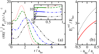
Figure 1: (Color online) (a) The dotted, dashed, dash-dotted and dash-dot-dotted lines show the scaled pair distribution function $r^{2}P_{12}(r)$ for $k_{B}T/(\hbar\omega)=0,0.6,1.2$ and $2$, respectively, for the $(3,1)$ system interacting through $V_{\text{G}}$ with $r_{0}=0.06a_{\text{ho}}$. The $T=0$ curve is determined using the basis set expansion approach while the finite $T$ curves are determined using the PIMC approach. The thick solid lines in the inset of panel (a), which is a blow-up of the small $r$ region, show the extrapolation to $r=0$. (b) The solid and dotted lines show the relative energy of the ground state with $L^{\Pi}=1^{-}$ and first excited state with $L^{\Pi}=0^{+}$ of the $(2,1)$ system interacting through $V_{\text{G}}$ with $r_{0}=0.06a_{\text{ho}}$ as a function of $-1/a_{s}$.

shows the scaled pair distribution function $r^{2}P_{12}(r)$ for the $(3,1)$ system for four temperatures, $k_{B}T/E_{\text{ho}}=0$, $0.6$, $1.2$ and $2$. At $T=0$ [dotted line in Fig. 1(a)], $P_{12}$ is governed by the lowest eigenstate, which has $L^{\Pi}=1^{+}$ symmetry rakshit12 ($L$ and $\Pi$ denote the orbital angular momentum and parity, respectively). As the temperature increases, excited states contribute. The second lowest state has $1^{-}$ symmetry. Compared to the ground state, its $P_{12}$ has an increased amplitude in the small but finite $r$ region. The scaled pair distribution function $r^{2}P_{12}$ for $k_{B}T=0.6E_{\text{ho}}$ (dashed line) has a comparable amplitude to that for $T=0$; however, clear differences are visible at larger interspecies distances $r$. For yet larger $T$, the small $r$ amplitude decreases drastically [see dash-dotted and dash-dot-dotted lines in Fig. 1(a)] while the maximum of $r^{2}P_{12}$ moves to larger $r$. To extract the contact from $r^{2}P_{12}$, we fit the small $r$ region ($r$ larger than $r_{0}$) and extrapolate the fit to $r=0$ [see thick solid lines in the inset of Fig. 1(a)].

Figure 2 shows the contact

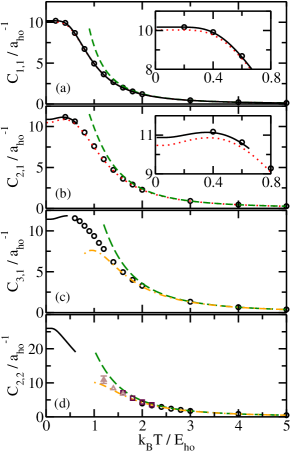
Figure 2: (Color online) Contact $C_{N_{1},N_{2}}$ as a function of $k_{B}T/E_{\text{ho}}$ for the (a) $(1,1)$, (b) $(2,1)$, (c) $(3,1)$, and (d) $(2,2)$ systems. The circles, squares and triangles show $C_{N_{1},N_{2}}$ for $V_{\text{G}}$ with $r_{0}/a_{\text{ho}}=0.06$, $0.08$ and $0.1$ obtained using the PIMC approach. The solid lines show $C_{N_{1},N_{2}}$ for $V_{\text{G}}$ with $r_{0}=0.06a_{\text{ho}}$ obtained using the basis set expansion approach. For comparison, the dotted lines in panels (a) and (b) show $C_{N_{1},N_{2}}$ obtained using $V_{\text{F}}$. (a) The dashed line shows the first-order Taylor expansion at high temperature. (b) The dashed line shows the cluster expansion, i.e., the quantity $2C_{1,1}$. (c)/(d) The dashed and dash-dotted lines show the leading order term of the cluster expansion and the full cluster expansion, respectively. The insets of panels (a) and (b) show blow-ups of the low temperature regions.

$C_{N_{1},N_{2}}$ at unitarity for $N=2-4$ as a function of the temperature. The symbols show the PIMC results, obtained by analyzing the scaled pair distribution functions $r^{2}P_{12}(r)$ for $V_{\text{G}}$ with $r_{0}\ll a_{\text{ho}}$. The solid lines in Fig. 2 show the contact for $r_{0}=0.06a_{\text{ho}}$ obtained by evaluating the adiabatic relation via the microscopic approach. It can be seen that the contact calculated by evaluating the adiabatic relation via the microscopic approach and the pair relation via the direct approach agree or connect smoothly for the three system sizes considered.

To estimate the dependence of the contact on the range $r_{0}$ of the underlying two-body potential, we determine the contact of the $(1,1)$ and $(2,1)$ systems with zero-range interactions (see supplemental material). The dotted lines in Figs. 2(a) and 2(b) show the result. In the low temperature regime, the contact for $r_{0}=0$ lies below that for $r_{0}>0$ for the $(1,1)$ and $(2,1)$ systems. At $k_{B}T=0.4E_{\text{ho}}$, e.g., the $(1,1)$ and $(2,1)$ contacts for $r_{0}=0.06a_{\text{ho}}$ lie 1.5% and 3%, respectively, above the contact for $r_{0}=0$. At large $T$, the dependence of the contact on the range is negligibly small. Our PIMC simulations suggest a similar range dependence for the $(3,1)$, $(4,1)$ and $(2,2)$ systems.

Figures 2(a)-2(d) show an intriguing dependence of the contact on the temperature. $C_{1,1}$ and $C_{2,2}$ decrease monotonically with increasing temperature while $C_{2,1}$ and $C_{3,1}$ exhibit a maximum at $k_{B}T\approx 0.36E_{\text{ho}}$ and between $0.4E_{\text{ho}}$ and $0.5E_{\text{ho}}$, respectively. To explain this behavior, it is instructive to evaluate the adiabatic relation via the microscopic approach.

For the $(1,1)$ system with zero-range interactions, one finds $\partial E_{j}/(\partial(-a_{s}^{-1}))=\Gamma(j+1/2)2^{3/2}/[\pi(2j)!]E_{\text{ho}}a_{\text{ho}}$ for the $s$-wave states and $\partial E_{j}/(\partial(-a_{s}^{-1}))=0$ for all higher partial wave states busch ; blume12 . The fact that $C_{1,1}$ decreases monotonically with decreasing temperature is thus a direct consequence of the fact that $\partial E_{j}/(\partial(-a_{s}^{-1}))$ (for $s$-wave states) decreases with increasing $j$. The inclusion of effective range corrections does not, if applied to the Gaussian model interaction with sufficiently small $r_{0}$, change this picture supplement . A similar analysis, based on the numerically determined energies, holds for the $(2,2)$ system. Figure 1(b) shows the lowest two relative eigen energies, which correspond to states with $L^{\Pi}=1^{-}$ and $0^{+}$ symmetry, respectively, of the $(2,1)$ system as a function of $-a_{\text{ho}}/a_{s}$ for $r_{0}=0.06a_{\text{ho}}$. The slope of the $1^{-}$ state is smaller than that of the $0^{+}$ state. This can be understood as follows. In the $a_{s}\rightarrow 0^{-}$ limit, the lowest state has $L^{\Pi}=1^{-}$ symmetry. In the $a_{s}\rightarrow 0^{+}$ limit, in contrast, the lowest state has $L^{\Pi}=0^{+}$ symmetry. The two states cross at $a_{\text{ho}}/a_{s}\approx 1$  kestner ; kolck ; stecher . Correspondingly, in the unitary regime the energy of the lowest $L=0$ state changes more rapidly with $-1/a_{s}$ than that of the lowest $L=1$ state, implying that the contact at unitarity increases in the low temperature regime where the inclusion of only two states yields converged results. A more comprehensive analysis that accounts for all states is presented in the supplemental material supplement . For the $(3,1)$ system, a similar argument can be made in the low temperature regime where the inclusion of just a few states suffices. The calculations presented here suggest that $C_{N_{1},N_{2}}$ decreases monotonically with $T$ if $N_{1}-N_{2}=0$ and exhibits a maximum at finite $T$ if $N_{1}-N_{2}\neq 0$. While it is tempting to generalize these results to larger systems, it should be noted that the density of states increases dramatically with increasing $N$ and that application of a few-state model will be limited to smaller temperatures as $N$ increases.

We now introduce a high temperature cluster expansion of the contact at unitarity. A formal discussion of the cluster expansion in the canonical ensemble applied to classical systems is provided in Ref. mathpaper . The $(N_{1},N_{2})$ system contains $N_{1}N_{2}$ interacting pairs and one might expect that, using the argument that two-component Fermi gases behave universally giorginiReview ; blumerev , the high temperature tail of $C_{N_{1},N_{2}}$ is governed by $N_{1}N_{2}C_{1,1}$ for $k_{B}T\gg E_{\text{ho}}$ [see dashed lines in Figs. 2(b)-2(d)]. The next term in the cluster expansion, applicable to systems with $N>3$, depends on the “three-body term” $C_{2,1}-2C_{1,1}$,

$$\frac{C_{N_{1},N_{2}}}{N_{1}N_{2}}=C_{1,1}+\frac{N_{1}+N_{2}-2}{2}(C_{2,1}-2C_{1,1})+\cdots.$$ (4)

The dashed and dash-dotted lines in Figs. 2(c) and 2(d) show the leading term and the sum of the leading and sub-leading terms for the $(3,1)$ and $(2,2)$ systems. The inclusion of the three-body term improves the validity regime of the cluster expansion notably. Assuming zero-range interactions, the leading order terms of the Taylor expansions of $C_{1,1}$ and $C_{2,1}-2C_{1,1}$ around $\tilde{\omega}\ll 1$, where $\tilde{\omega}=E_{\text{ho}}/(k_{B}T)$, are $4\pi^{1/2}\tilde{\omega}^{5/2}a_{\text{ho}}^{-1}$ and $-7.012(12)\tilde{\omega}^{11/2}a_{\text{ho}}^{-1}$, indicating that the three-body term is suppressed by $\tilde{\omega}^{3}$ compared to the leading order two-body term. Figures 2(c) and 2(d) show that the numerically obtained $C_{3,1}$ and $C_{2,2}$ contacts (symbols) lie above the cluster prediction (dash-dotted line), suggesting that the corresponding leading order four-body expansion coefficients are positive. The above expansions can be viewed as canonical analogs of the virial equation of state description of the contact within the grand canonical ensemble liurev ; liuNJP ; supplement .

Equation (4) shows that the contact $C_{N-1,1}$ with $N>2$ is $N-1$ times larger than $C_{1,1}$ in the high temperature limit. In the low temperature limit (see Fig. 3),

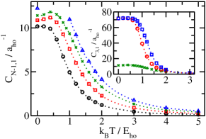
Figure 3: (Color online) Circles, squares, crosses and triangles show $C_{N_{1},N_{2}}$ for the $(1,1)$, $(2,1)$, $(3,1)$ and $(4,1)$ systems, respectively, interacting through $V_{\text{G}}$ with $r_{0}=0.06a_{\text{ho}}$ as a function of $T$ footnote41system . Dotted lines serve as a guide to the eye. Inset: Crosses, squares and circles show the contact of the $(3,1)$ system for Fermi, Boltzmann and Bose statistics, respectively.

in contrast, $C_{N-1,1}$ with $N>2$ is only slightly larger than $C_{1,1}$, reflecting the fact that, to leading order, the system can form one and not $N-1$ bound pairs. It is also interesting to compare the limiting behaviors of $C_{3,1}$ and $C_{2,2}$. $C_{2,2}$ is $4/3$ times larger than $C_{3,1}$ at large $T$ [see Eq. (4)] but roughly two times larger at low $T$. The latter reflects the fact that the $(2,2)$ and $(3,1)$ systems can form two dimers and one dimer, respectively.

To elucidate the role of the Fermi statistics, we focus on the $(3,1)$ system at unitarity with $r_{0}=0.06a_{\text{ho}}$. The inset of Fig. 3 shows the contact obtained by treating the majority particles as identical fermions (crosses; these are the same data as discussed above), as identical bosons (circles) and as distinguishable “Boltzmann particles” (squares). In the high temperature regime, the Fermi and Bose statistics can be treated as a correction to the Boltzmann statics. In the low temperature regime, in contrast, appreciable differences are revealed. The $(3,1)$ systems with Bose and Boltzmann statistics share the same ground state and thus the same contact in the zero temperature limit. Compared to the contact of the Bose and Boltzmann systems, that of the Fermi system is strongly suppressed as a consequence of the Pauli exclusion principle. Specifically, the $(3,1)$ Fermi system at unitarity does not support a bound state in free space while the $(3,1)$ Bose and Boltzmann systems do. The existence of self-bound states leads to an increased amplitude of the pair distribution function at small interspecies distances. Moreover, the Bose and Boltzmann systems are—unlike the Fermi system—not fully universal, i.e., their properties are, in addition to the $s$-wave scattering length, governed by a three-body parameter. This implies that the Bose and Boltzmann systems are characterized by a non-zero three-body contact in addition to the two-body contact considered throughout this paper BraatenPlatter ; footnote1 .

Finite-temperature effects play an important role in many finite-sized systems, including atomic clusters, nuclei and quantum dots. Our work demonstrates that small harmonically trapped two-component Fermi gases with infinitely strong interspecies $s$-wave interactions, which can be realized and probed experimentally, also exhibit intriguing dependencies on the temperature. In particular, we proposed a high-temperature cluster expansion in the canonical ensemble, quantified the range dependence of the contact, observed and interpreted the distinctly different behavior of the contact of spin-balanced and spin-imbalanced Fermi gases in the low temperature regime, and elucidated the role of the Fermi statistics. Throughout, we reported the temperature in terms of the natural energy scale of the harmonic oscillator. Other relevant temperature scales are the Fermi temperature $T_{F}$ and the critical temperature $T_{c}$, $T_{F}=2.5E_{\text{ho}}/k_{B}$ for $N=3-5$ footnotetf and $T_{c}\approx 0.2T_{F}$ for the trapped spin-balanced system Stringari13 . Our calculations cover temperatures much smaller and much larger than these characteristic temperature scales. Future studies will be aimed at determining the critical temperature, and the superfluid fraction and superfluid density of small trapped Fermi gases.

Support by the National Science Foundation (NSF) through Grant No. PHY-1205443 is gratefully acknowledged. This work used the Extreme Science and Engineering Discovery Environment (XSEDE), which is supported by NSF grant number OCI-1053575, and the WSU HPC. This work was additionally supported by the NSF through a grant for the Institute for Theoretical Atomic, Molecular and Optical Physics at Harvard University and Smithsonian Astrophysical Observatory.

References

- (1) S. Tan, Ann. Phys. 323, 2952 (2008).
- (2) S. Tan, Ann. Phys. 323, 2971 (2008).
- (3) S. Tan, Ann. Phys. 323, 2987 (2008).
- (4) F. Werner and Y. Castin, Phys. Rev. A 86, 013626 (2012).
- (5) E. Braaten and L. Platter, Phys. Rev. Lett. 100, 205301 (2008).
- (6) J. T. Stewart, J. P. Gaebler, T. E. Drake, and D. S. Jin, Phys. Rev. Lett. 104, 235301 (2010).
- (7) E. D. Kuhnle, H. Hu, X.-J. Liu, P. Dyke, M. Mark, P. D. Drummond, P. Hannaford, and C. J. Vale, Phys. Rev. Lett. 105 070402 (2010).
- (8) E. D. Kuhnle, S. Hoinka, P. Dyke, H. Hu, P. Hannaford, and C. J. Vale, Phys. Rev. Lett. 106 170402 (2011).
- (9) Y. Sagi, T. E. Drake, R. Paudel, and D. S. Jin, Phys. Rev. Lett. 109, 220402 (2012).
- (10) S. Hoinka, M. Lingham, K. Fenech, H. Hu, C. J. Vale, J. E. Drut, and S. Gandolfi, Phys. Rev. Lett. 110, 055305 (2013).
- (11) D. Blume and K. M. Daily, Phys. Rev. A 80, 053626 (2009)
- (12) F. Werner, L. Tarruell, and Y. Castin, Eur. Phys. J. B 68, 401 (2009).
- (13) F. Palestini, A. Perali, P. Pieri, and G. C. Strinati, Phys. Rev. A 82, 021605(R) (2010).
- (14) J. E. Drut, T. A. Lähde, and T. Ten, Phys. Rev. Lett. 106, 205302 (2011).
- (15) K. Van Houcke, F. Werner, E. V. Kozik, N. V. Prokof’ev, and B. V. Svistunov, arXiv:1303.6245.
- (16) I. Boettcher, S. Diehl, J. M. Pawlowski, and C. Wetterich, Phys. Rev. A 87, 023606 (2013).
- (17) M. Barth and W. Zwerger, Ann. Phys. 326, 2544 (2011).
- (18) E. V. H. Doggen and J. J. Kinnunen, arXiv:1304.0918.
- (19) T.-L. Ho and E. J. Mueller, Phys. Rev. Lett. 92, 160404 (2004).
- (20) X.-J. Liu, H. Hu, and P. D. Drummond, Phys. Rev. Lett. 102, 160401 (2009).
- (21) X.-J. Liu, Phys. Rep. 524, 37 (2013).
- (22) K. Huang and C. N. Yang, Phys. Rev. 105, 767 (1957).
- (23) T. Busch, B.-G. Englert, K. Rza̧żewski, and M. Wilkens, Found. Phys. 28, 549 (1998).
- (24) F. Werner and Y. Castin, Phys. Rev. Lett. 97, 150401 (2006).
- (25) Y. Suzuki and K. Varga. Stochastic Variational Approach to Quantum Mechanical Few-Body Problems. Springer Verlag, Berlin (1998).
- (26) K. M. Daily and D. Blume, Phys. Rev. A 81, 053615 (2010).
- (27) D. Rakshit, K. M. Daily, and D. Blume, Phys. Rev. A 85, 033634 (2012).
- (28) D. M. Ceperley, Rev. Mod. Phys. 67, 279 (1995).
- (29) see, e.g., D. M. Ceperley, J. Stat. Phys. 63, 1237 (1991).
- (30) K. M. Daily, X. Y. Yin, and D. Blume, Phys. Rev. A 85, 053614 (2012).
- (31) See the supplemental material at www.to.be.inserted.by.the.editor for details.
- (32) J. P. Kestner and L.-M. Duan, Phys. Rev. A 76, 033611 (2007).
- (33) I. Stetcu, B. R. Barrett, U. van Kolck, and J. P. Vary, Phys. Rev. A 76, 063613 (2007).
- (34) J. von Stecher, D. Blume, and C. H. Greene, Phys. Rev. A 77, 043619 (2008).
- (35) E. Pulvirenti and D. Tsagkarogiannis, Commun. Math. Phys. 316, 289 (2012).
- (36) S. Giorgini, L. P. Pitaevskii, and S. Stringari, Rev. Mod. Phys. 80, 1215 (2008).
- (37) D. Blume, Rep. Prog. Phys. 75, 046401 (2012).
- (38) H. Hu, X.-J. Liu, and P. D. Drummond, New J. Phys. 13, 035007 (2011).
- (39) For the system, the results derived from the basis set expansion approach cover the temperature range . The results derived from the PIMC approach cover the temperature range . For this system, we did not treat the temperature regime between . Nevertheless, our results suggest that exhibits a maximum at finite , like the other maximally polarized systems considered in this paper.
- (40) The three-body contact BraatenPlatter should not be confused with the two-body contact of the two-, three- and higher-body systems. For the Fermi systems considered in this work, the three-body contact vanishes identically.
- (41) E. Braaten, D. Kang and L. Platter, Phys. Rev. Lett. 106, 153005 (2011).
- (42) The Fermi temperature of small harmonically trapped two-component Fermi gases is defined through the energy of the highest single-particle state of the non-interacting system.
- (43) L. A. Sidorenkov, M. K. Tey, R. Grimm, Y.-H. Hou, L. Pitaevskii, and S. Stringari, arXiv:1302.2871.