Renormalization Group Approach to Dissipative System

School of Food and Nutritional Sciences, University of Shizuoka,
Yada 52-1, Shizuoka 422-8526, Japan
Corresponding author: ichinose@u-shizuoka-ken.ac.jp

1 Introduction

In order to understand the dynamical mechanism of the friction phenomena, we heavily rely on the numerical analysis using various methods: molecular dynamics, Langevin equation, lattice Boltzmann method, Monte Carlo, e.t.c.. For the case of the Langevin equation, for example, a simple model is described as follows.

$$m\ddot{x}=-{\eta}\dot{x}-\frac{\partial V}{\partial x}+{\mbox{random force}}{\quad,}$$

$${\eta}\ :\ \mbox{viscosity},\ \ V(x):\ \mbox{potential}{\quad.}$$ (1)

The effect of the random force is given by the white noise. We propose a new method which has the following characteristic points: 1) the geometrical approach to the statistical mechanical system; 2) the continuum approach using Feynman’s path integral (generalized version); 3) the holographic (higher-dimensional) approach; 4) the renormalization phenomenon takes place in order to treat the statistical fluctuation.

In ref.[1, 2], we have explained this method using the above model (1).

2 One Dimensional Spring-Block Model

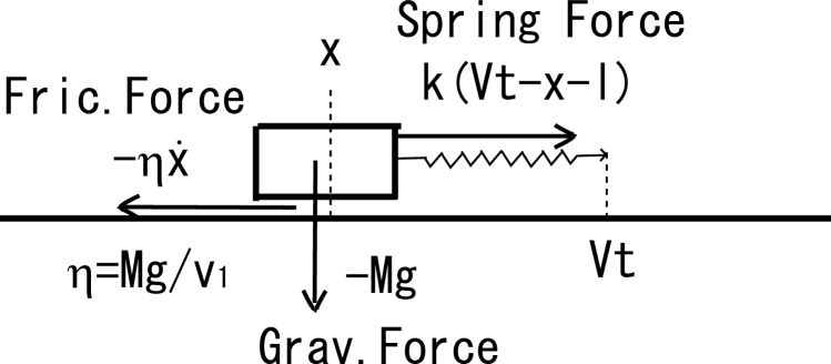
Figure 1: One dimensional spring-block model

We take another simple model of the friction system: the spring-block model. See Fig.1. It describes the movement of a block (rigid body), dragged by the spring, on a table with friction. The front end of the spring moves with the constant velocity $V$. The equation of motion is given by

$$M\ddot{x}=-\mu(\dot{x})Mg+k(Vt-x-l),\ \mu(\dot{x})=\frac{1}{v_{1}}\dot{x}\ ,$$ (2)

where $M$ is the mass, $\mu$ is the friction coefficient, $g$ is the gravitational acceleration constant, $k$ is the spring constant, $V$ is the front-end velocity (constant), and $l$ is the natural length of the spring. It can be re-written as

$$\ddot{x}+\frac{1}{\tau_{1}}\dot{x}+\omega^{2}x=\omega^{2}(Vt-l),\ \tau_{1}\equiv\frac{v_{1}}{g},\ \omega\equiv\sqrt{\frac{k}{M}}\ .$$ (3)

For the initial condition: $x(0)=-l\ ,\ \dot{x}(0)=0$, the classical solution (elasticity dominate case, $4\omega^{2}>1/{\tau_{1}}^{2}$) is given by

$$x(t)={\rm e}^{-t/2\tau_{1}}V\{(1/2\omega^{2}\tau_{1}^{2}-1)(\sin\Omega t)/\Omega+(1/\omega^{2}\tau_{1})\cos\Omega t\}$$

$$-l+V(t-1/\omega^{2}\tau_{1}),\ \ \Omega=(1/2)\sqrt{4\omega^{2}-1/{\tau_{1}}^{2}},$$

$$0\leq t\leq 2,\ x(0)=-l,\ \dot{x}(0)=0.$$ (4)

See Fig.2. It shows the ’stick-slip’ motion. The time interval for one pair of the stick and slip-state is $2\pi/\Omega$.

Figure 2: The solution (4) with $\tau_{1}=V=l=1.0,\omega=10.0,\Omega=\sqrt{399}/2,0\leq t\leq 2$.

We impose the periodicity on the t-axis for the (IR) regularization. (Physically this procedure is regarded as putting the whole system in the heat-bath of the temperature $\beta^{-1}$. )

$$t\ \rightarrow\ t+\beta,\ \beta^{-1}:\ \mbox{temperature}.$$ (5)

The equation of motion (3) gives us the following relation.

$$\left[{1\over 2}\dot{x}^{2}+\frac{\omega^{2}}{2}x^{2}+\omega^{2}lx\right]_{t_{1}}^{t_{2}}=-\frac{1}{\tau_{1}}\int_{t_{1}}^{t_{2}}\dot{x}^{2}dt+\omega^{2}V\int_{t_{1}}^{t_{2}}t\dot{x}dt.$$ (6)

Changing variables $t_{2}$ to $t$, and $t_{1}$ to $0$, we read the energy conservation equation.

$$H[\dot{x},x]\equiv{1\over 2}\dot{x}^{2}+\frac{\omega^{2}}{2}x^{2}+\omega^{2}lx+\frac{1}{\tau_{1}}\int_{0}^{t}\dot{x}^{2}d{\tilde{t}}-\omega^{2}V\int_{0}^{t}{\tilde{t}}\dot{x}d{\tilde{t}}$$

$$=\left({1\over 2}\dot{x}^{2}+\frac{\omega^{2}}{2}x^{2}+\omega^{2}lx\right)_{t=0}=-\frac{\omega^{2}}{2}l^{2}=E_{0}\ (\mbox{constant}){\quad,}$$ (7)

where we have used the initial condition: $x(0)=-l\ ,\ \dot{x}(0)=0$. In the second formula, the fourth and the fifth terms are the hysteresis ones, $\{x({\tilde{t}}):\ 0\leq{\tilde{t}}\leq t\}$. The fourth term is the friction-heat energy produced until the time $t$. The fifth one is the subtraction of the cumulated external work done by the dragging until the time $t$. From this Hamiltonian (energy) expression, (7), we can read the (bulk) metric in the 2 dimensional (D) space $(X,t)$.[1] There are two types.

Dirac Type

$$ds^{2}\mbox{}_{D}\equiv dX\mbox{}^{2}+(\omega^{2}X^{2}+2\omega^{2}lX)\leavevmode\nobreak\ dt\mbox{}^{2}$$

$$+dt\mbox{}^{2}\left\{\frac{2}{\tau_{1}}\int_{-l}^{x(t)}\dot{X}dX-2\omega^{2}V\int_{-l}^{x(t)}{\tilde{t}}\leavevmode\nobreak\ dX\right\},$$ (8)

where $0\leq{\tilde{t}}\leq t$ and $\dot{X}=\frac{dX}{d{\tilde{t}}}$. From this construction of the bulk metric, we see $ds^{2}\mbox{}_{D}$ reduces, on a path $X=x(t)$, to be proportional to the energy. On a path

$$X=x(t),\ 0\leq t\leq\beta,\ dX=\dot{x}dt,$$ (9)

the induced metric is given by

$$ds^{2}\mbox{}_{D}|_{on-path}=\left[\dot{x}^{2}+\omega^{2}x^{2}+2\omega^{2}lx\right.$$

$$\left.+\frac{2}{\tau_{1}}\int_{0}^{t}\dot{x}^{2}d{\tilde{t}}-2\omega^{2}V\int_{0}^{t}{\tilde{t}}\dot{x}d{\tilde{t}}\right]dt\mbox{}^{2}\equiv 2H[\dot{x},x]dt\mbox{}^{2}.$$ (10)

The length $L$ of the path $\{x(t)|0\leq t\leq\beta\}$ is given by

$$L[x(t)]=\int ds=\int_{0}^{\beta}\sqrt{2H}dt.$$ (11)

Standard Type
We take the following form for the line element $ds^{2}\mbox{}_{S}$.

$$ds^{2}\mbox{}_{S}=\frac{1}{dt\mbox{}^{2}}(ds^{2}\mbox{}_{D})^{2}\ -\ \mbox{on-path}\ \rightarrow\ (2H[\dot{x},x])^{2}dt\mbox{}^{2}.$$ (12)

On the path, the length is given by

$$L[x(t)]=2\int_{0}^{\beta}H[\dot{x},x]dt.$$ (13)

The spring-block starts with the stick-slip motion and finally reaches the steady state with a constant velocity. During the movement the friction-heat is produced and the external work, by the dragging, keeps being given. Microscopically the statistical fluctuation occurs in the (bottom) surface of the block. For both types of metric, the free energy $F$ is given by the path-integral [3] with the statistical weight $\exp(-L/2\alpha^{\prime})$ (the statistical ensemble measure based on the geometry[1, 4]).

$${\rm e}^{-\beta F[l,\alpha^{\prime},\beta;\omega,\tau_{1},V]}=\int_{-l}^{\beta V}d\rho\int_{\begin{array}[]{c}x(0)=-l\\ x(\beta)=\rho\end{array}}$$ (16)

$$\times\prod_{t}{\cal D}x(t)\exp\left[-\frac{1}{2\alpha^{\prime}}L[x(t)]\right].$$ (17)

The paths are shown in Fig.3. $\alpha^{\prime}$ is a new model parameter which shows the tension of the 1D string (line). The parameter $\alpha^{\prime}$ has the dimension of length ($[\alpha^{\prime}]=\mbox{L}$) for Dirac-type, while that of Standard-type has the dimension of length$\times$velocity ($[\alpha^{\prime}]\ ={\mbox{L}}^{2}/{\mbox{T}}$). $\beta^{-1}$ is regarded as the temperature of the final (equilibrium) state.

The energy E, and the entropy S are obtained by

$$\mbox{Energy}\ E(l,\alpha^{\prime},\beta;\omega,\tau_{1},V)=<\frac{L}{2}>=\frac{\partial}{\partial(-{\alpha^{\prime}}^{-1})}{\rm e}^{-\beta F},$$

$$\mbox{Entropy}\quad S(l,\alpha^{\prime},\beta;\omega,\tau_{1},V)=k\beta(E-F).$$ (18)

The effective force emerges, as the statistically averaging effect, in the spring-block and is given by

$$\mbox{Force}\quad f(l,\alpha^{\prime},\beta;\omega,\tau_{1},V)=-\frac{\partial E}{\partial l}$$ (19)

Evaluation of the free energy, (17), requires the renormalization of some parameters.

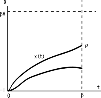
Figure 3: The paths appearing in the path-integral expression (17) of the free energy during the movement of the block.

3 Two Dimensional Dissipative Block in the Central Force

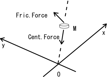
Figure 4: 2D dissipative block in the central force

We consider the case that a block moves on a plane, described by the coordinates ${\bf x}=(x,y)$, with the friction under the influence of the central force.

$$M\ddot{{\bf x}}=-\mu(\dot{{\bf x}})Mg\frac{\dot{{\bf x}}}{|\dot{{\bf x}}|}+F(|{\bf x}|)\frac{{\bf x}}{|{\bf x}|},M:\mbox{mass};\ g:\mbox{grav. accel.}$$

$$\mbox{Fric. Coeff.};\ \mu(\dot{{\bf x}})=\frac{|\dot{{\bf x}}|}{v_{1}},\ \mbox{Cent. Force}:\ F=-k|{\bf x}|.$$ (20)

The classical equation of motion is expressed as

$$\ddot{{\bf x}}+\frac{1}{\tau_{1}}\dot{{\bf x}}+\omega^{2}{\bf x}=0,\ \omega^{2}=\frac{k}{M},\ \tau_{1}=\frac{v_{1}}{g}.$$ (21)

In terms of the polar coordinates $(r,\theta)$, this equation is re-written as

$${\bf x}=(x=r\cos\theta,y=r\sin\theta){\quad,}$$

$$\ddot{r}+\frac{1}{\tau_{1}}\dot{r}-r(\dot{\theta}^{2}-\omega^{2})=0{\quad,}\quad r\ddot{\theta}+(2\dot{r}+\frac{r}{\tau_{1}})\dot{\theta}=0{\quad.}$$ (22)

A solution (central-force dominant case: $\omega^{2}>\frac{1}{4{\tau_{1}}^{2}}$) is given by

$$r(t)={\rm e}^{-\frac{t}{2\tau_{1}}}r_{0}(\sin\omega_{0}t\ +1){\quad,}$$

$$\theta(t)={1\over 2}\tan(\frac{\omega_{0}t}{2}-\frac{\pi}{4})+\frac{1}{6}\tan^{3}(\frac{\omega_{0}t}{2}-\frac{\pi}{4})+\frac{2}{3}{\quad,}$$ (23)

where $r_{0}$ and $\omega_{0}$ are the parameters appearing in the initial condition $r(0)=r_{0},\theta(0)=\theta_{0},v_{r}(0)={v_{r}}^{0}$ and $\dot{\theta}(0)=\omega_{0}$ which we choose in the following way.

$$\omega_{0}=\sqrt{\omega^{2}-\frac{1}{4{\tau_{1}}^{2}}}{\quad,}\quad\frac{{v_{r}}^{0}}{r_{0}}=-\frac{1}{2\tau_{1}}+\sqrt{\omega^{2}-\frac{1}{4{\tau_{1}}^{2}}}{\quad,}\quad\theta_{0}=0{\quad.}$$ (24)

The choice (24) is only for the simple form of (23). For the case $\tau_{1}=1,\omega=1$ and $r_{0}=1$, the orbit is shown in Fig.5 for $-0.2\leq x\leq 1.2$ and in Fig.6 for $-0.1\leq x\leq 0.1$. The orbit shows ’stick-slip’ motion and the time interval for the one motion is $2\pi/\dot{\theta}(0)$.

Figure 5: Movement of 2D spring-block model. $\tau_{1}=1,\omega=1;\ \dot{\theta}(0)=\sqrt{3/4},\theta(0)=0,r(0)=1,\dot{r}(0)=(\sqrt{3}-1)/2.\ \ -0.2\leq x\leq 1.2,\ \ -0.1\leq y\leq 0.6$

Figure 6: Movement of 2D spring-block model. $\tau_{1}=1,\omega=1;\ \dot{\theta}(0)=\sqrt{3/4},\theta(0)=0,r(0)=1,\dot{r}(0)=(\sqrt{3}-1)/2.\ \ -0.1\leq x\leq 0.1,\ \ -0.05\leq y\leq 0.1$

As in Sec.2, we impose the periodicity on t-axis: $t\rightarrow t+\beta$. From the equation of motion (21) we can derive the following relation.

$$\left[{1\over 2}{\dot{{\bf x}}}^{2}+\frac{\omega^{2}}{2}{\bf x}^{2}\right]^{t}_{0}=-\frac{1}{\tau_{1}}\int^{t}_{0}{\dot{{\bf x}}}^{2}d{\tilde{t}},\ \omega^{2}=\frac{k}{M},\ \tau_{1}=\frac{v_{1}}{g},$$ (25)

where $0\leq t\leq\beta$. From this result, we obtain the energy conservation equation.

$$H[\dot{{\bf x}},{\bf x}]\equiv{1\over 2}{\dot{{\bf x}}}^{2}+\frac{\omega^{2}}{2}{\bf x}^{2}+\frac{1}{\tau_{1}}\int^{t}_{0}{\dot{{\bf x}}}^{2}d{\tilde{t}}=\left({1\over 2}{\dot{{\bf x}}}^{2}+\frac{\omega^{2}}{2}{\bf x}^{2}\right)|_{t=0}=E_{0},$$ (26)

where the third term of the second formula shows the hysteresis effect and $\dot{{\bf x}}=d{\bf x}({\tilde{t}})/d{\tilde{t}}\ ,\ 0\leq{\tilde{t}}\leq t$. From the above equation, we can read the 3 dim (bulk) metric.

$$\mbox{Dirac}:\ ds^{2}\mbox{}_{D}\equiv d{\bf X}\mbox{}^{2}+\omega^{2}{\bf X}^{2}dt^{2}+\frac{2}{\tau_{1}}dt^{2}\int^{{\bf X}(t)}_{{\bf X}_{0}}\dot{{\bf X}}\cdot d{\bf X},$$

$$\mbox{Standard}:\ ds^{2}\mbox{}_{S}\equiv\frac{1}{dt^{2}}(ds^{2}\mbox{}_{D})^{2},$$ (27)

where $\dot{{\bf X}}=\frac{d{\bf X}({\tilde{t}})}{d{\tilde{t}}},\ 0\leq{\tilde{t}}\leq t,\ {\bf X}_{0}\equiv{\bf X}(0)$. The friction occurs between the top surface of the plane and the bottom surface of the block. The solution (23) shows that the block does the stick-slip motion. The friction is microscopically caused by the irregularly-distributed asperity on both surfaces. We introduce the distribution of the movement-configuration in the geometrical way. In order to define it, we first prepare the following 2D surface in the 3 dimensional (bulk) space ($t,X,Y$).

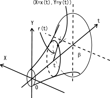
Figure 7: 2D surface embedded in 3D space-time by the closed-string condition (28).

$$\mbox{Closed-String Condition}:$$

$${\bf x}^{2}(t)=x(t)^{2}+y(t)^{2}=r(t)^{2},\ 0\leq t\leq\beta,$$ (28)

where we assume the 2D world described by the coordinates ($x,y$) is isotropic around the origin. See Fig.7. The function form of $r(t)$ can be taken in the arbitrary way. The configuration is a closed-string. $\beta$ is a boundary parameter of $t$-axis. It plays the role of the inverse temperature of the final (equilibrium) state of the system. The metric on the surface, called ”induced metric”, is obtained by using the closed-string condition (28) in the expression (27).

$$ds^{2}\mbox{}_{D}|_{on-path}=$$

$$dr^{2}+r^{2}d\theta^{2}+\frac{dr^{2}}{\dot{r}^{2}}\left\{\omega^{2}r^{2}+\frac{2}{\tau_{1}}\int_{0}^{t}(\dot{r}^{2}+r^{2}\dot{\theta}^{2})d{\tilde{t}}\right\}$$

$$\equiv g^{ind}_{ij}dx^{i}dx^{j},\quad i,j=1,2;\ (x^{1},x^{2})=(r,\theta),$$ (29)

where $x(t)=r(t)\cos\theta(t),\ y(t)=r(t)\sin\theta(t)$. The induced metric is explicitly given by

$$g^{ind}_{ij}(r(t),\theta(t))=\left(\begin{array}[]{cc}\frac{2H_{r}}{\dot{r}^{2}}&0\\ 0&\frac{2H_{\theta}}{\dot{\theta}^{2}}\end{array}\right),\quad 2H[r,\dot{r},\dot{\theta}]=$$ (32)

$$\dot{r}^{2}+r^{2}\dot{\theta}^{2}+\omega^{2}r^{2}+\frac{2}{\tau_{1}}\int_{0}^{t}(\dot{r}^{2}+r^{2}\dot{\theta}^{2})d{\tilde{t}}=2H_{r}+2H_{\theta}\ ,$$ (33)

where $2H_{\theta}\equiv r^{2}\dot{\theta}^{2}$ is the angular part of Hamiltonian and $2H_{r}\equiv 2H-2H_{\theta}$ is the radial one. The area $A$ of the surface is given by

$$A[r(t),\theta(t)]=\int\sqrt{\mbox{det}\leavevmode\nobreak\ g^{ind}_{ij}}\leavevmode\nobreak\ d^{2}x=$$

$$\int_{0}^{\beta}dt\int d\theta(t){\tilde{A}}[r(t),\theta(t)],\ {\tilde{A}}=2\leavevmode\nobreak\ \frac{\sqrt{H_{r}H_{\theta}}}{|\dot{\theta}|},$$ (34)

where $d^{2}x=dr\leavevmode\nobreak\ d\theta=\dot{r}d\theta dt$.

The macroscopic physical quantities, such as the energy of the whole system, are generally given by the form of the integral over the whole space-time (bulk space). They are often divergent[4, 5, 6]. In order to regularize the singular behavior, and to take the statistical average at the same time, we replace the integral by the sum (integral) over all possible surfaces satisfying the given boundary condition. The measure of the path (surface)-integral is taken as follows. An infinitesimal surface between $t$ and $t+dt$ is specified by $dr(t)=\dot{r}dt$ and $d\theta$. For simplicity, we consider the case: $\dot{\theta}=0,\theta=$constant. (The angular variable $\theta$ is commonly used for all $t$. ) The free energy $F$ is given by

$${\rm e}^{-\beta F[\rho_{0},\alpha^{\prime},\beta;\omega,\tau_{1}]}=\int_{\Lambda^{-1}}^{\mu^{-1}}d\rho\int_{\begin{array}[]{c}r(0)=\rho_{0}\\ r(\beta)=\rho\end{array}}\prod_{t^{\prime}}r(t^{\prime}){\cal D}r(t^{\prime})$$ (37)

$$\times\exp\left[-\frac{2\pi}{2\alpha^{\prime}}\int_{0}^{\beta}{\bar{A}}[r(t)]dt\right],{\bar{A}}[r(t)]=r\leavevmode\nobreak\ \sqrt{\dot{r}^{2}+\omega^{2}r^{2}+\frac{2}{\tau_{1}}\int_{0}^{t}\dot{r}^{2}d{\tilde{t}}\ }.$$ (38)

where $\Lambda^{-1}$ and $\mu^{-1}$ are the UV and IR regularization parameters. $\rho_{0}$ is a model parameter and shows the starting radial position. $\alpha^{\prime}$ is the parameter which shows the tension of the embedded 2D surface, Fig.7. Its physical dimension is  [$\alpha^{\prime}$]=L². The energy E, and the entropy S are obtained by

$$\mbox{Energy}:\ E(\rho_{0},\alpha^{\prime},\beta;\omega,\tau_{1})=<\frac{A}{2}>=\frac{\partial}{\partial(-{\alpha^{\prime}}^{-1})}{\rm e}^{-\beta F},$$

$$\mbox{Entropy}:\ S(\rho_{0},\alpha^{\prime},\beta;\omega,\tau_{1})=k\beta(E-F).$$ (39)

As the statistically averaging effect, the effective force emerges, in the radial direction, on the block and is given by

$$\mbox{Force}:\ f(\rho_{0},\alpha^{\prime},\beta;\omega,\tau_{1})=-\frac{\partial E}{\partial\rho_{0}}\ .$$ (40)

Evaluation of the free energy F, (38), requires the renormalization of some parameters.

4 Conclusion

Recently another new approach to the dissipative system is proposed[7], where the time development is replaced by the step-wise process. The present geometric approach is also applied to the condensed matter physics such as the permittivity of the substance[8].

We have proposed a new formalism to calculate the fluctuation effect in the dissipative system based on the geometry appearing in the system energy expression. The integration measure for the statistical ensemble is taken from Feynman’s idea of the path-integral. It clarifies the statistically-averaging procedure.

References

[1]S. Ichinose, J.Phys:Conf.Ser.258(2010)012003, arXiv:1010.5558,
Proc. of Int. Conf. on Science of Friction 2010
(Ise-Shima, Mie, Japan, 2010.9.13-18).
[2]S. Ichinose, arXiv:1004.2573,
”Geometric Approach to Quantum Statistical Mechanics and Minimal Area Principle”,
28pages.
[4] S. Ichinose,
Prog.Theor.Phys.121(2009)727, ArXiv:0801.3064v8[hep-th].
[5] S. Ichinose, ”Casimir Energy of 5D Warped System and Sphere Lattice Regularization”,
ArXiv:0812.1263[hep-th], US-08-03, 61 pages.
[6]S. Ichinose,
J. Phys. : Conf.Ser.384(2012)012028,
Proceedings of DSU2011 (2011.9.26-30, Beijin, China).
ArXiv:1205.1316[hep-th]
[7] S. Ichinose, ”Velocity-Field Theory, Boltzmann’s Transport Equation,
Geometry and Emergent Time”, arXiv:1303.6616(hep-th), 36 pages.
[8] S. Ichinose, ”Renormalization Group Approach to Casimir Effect and the Attractive and
Repulsive Forces in Substance”, Proc. Int. Tribology Conf. Hiroshima (Oct.30-Nov.3, 2011, Hiroshima,
Japan), arXiv:1203.2708(cond-mat), 18 pages.