Rosenbrock-Krylov Methods for Large Systems of Differential Equations

Abstract

This paper develops a new class of Rosenbrock-type integrators based on a Krylov space solution of the linear systems. The new family, called Rosenbrock-Krylov (Rosenbrock-K), is well suited for solving large-scale systems of ODEs or semi-discrete PDEs. The time discretization and the Krylov space approximation are treated as a single computational process, and the Krylov space properties are an integral part of the new Rosenbrock-K order condition theory developed herein. Consequently, Rosenbrock-K methods require a small number of basis vectors determined solely by the temporal order of accuracy. The subspace size is independent of the ODE under consideration, and there is no need to monitor the errors in linear system solutions at each stage. Numerical results show favorable properties of Rosenbrock-K methods when compared to current Rosenbrock and Rosenbrock-W schemes.

1 Introduction

This paper is concerned with the numerical solution of large initial value problems of the form

(1) $$\frac{dy}{dt}=f(t,y)\,,~{}~{}~{}t_{0}\leq t\leq t_{F}\,,~{}~{}~{}y(t_{0})=y_{0}\,;\quad y(t),f(t,y)\in\mathbb{R}^{N}\,.$$

Ordinary differential equations (ODEs) model the evolution of chemical kinetic systems, electronic circuits, or the motion of planets. Other physical systems, such as dynamics of the atmosphere and oceans, or the behavior of materials, require the solution of a system of partial differential equations (PDEs). A standard approach for solving evolutionary PDEs is to discretize in space, reducing the problem to a large system of ODEs which are then integrated forward in time.

The equations of interest in many simulations are driven by multiple physical processes, e.g., associated with the simulation of fluid-structure interaction, sub-grid-scale physics, or chemical reaction terms. These processes have different dynamical characteristics, with some being slow (e.g., transport) and some fast (e.g., stiff chemistry). In addition, multiple spatial and temporal scales are associated with non-uniform meshes, with boundary layers, with fast waves, and with the structure of the system (e.g., the existence of jet fans). The existence of fast and slow dynamics poses considerable challenges to the solution of the semi-discrete PDEs (1) by explicit time stepping methods. Specifically, due to the Courant-Friedrichs-Lewy (CFL) stability condition, the largest allowable step sizes are bounded above by the shortest (fastest) time scale in the system.

To avoid stability restrictions on the step size, implicit time integration methods are becoming widely used in the simulation of large-scale evolutionary PDEs (1). Implicit time stepping requires the solution of large nonlinear systems of equations, coupling all variables in the model, at each time step. The associated computation and communication costs constitute a major scalability bottleneck at best, and can quickly become infeasible for large systems.

In this paper we examine, and extend, the Rosenbrock class of integration methods. These are linearly-implicit methods which enjoy the benefit of requiring a fixed number of linear solves, as opposed to non-linear solves in the case of implicit Runge-Kutta methods. A general $s$-stage Rosenbrock method reads [13, Section IV.7]

(2a) $$y_{n+1} = y_{n}+\displaystyle\sum_{i=1}^{s}b_{i}\,k_{i}\,,$$

$$\qquad\left(\mathbf{I}_{N\times N}-h\,\gamma_{i,i}\,\mathbf{A}_{n}\right)\cdot k_{i} = h\,f\left(t_{n}+\alpha_{i}h,y_{n}+\displaystyle\sum_{j=1}^{i-1}\alpha_{i,j}\,k_{j}\right)$$

$$+h\,\mathbf{A}_{n}\,\displaystyle\sum_{j=1}^{i-1}\gamma_{i,j}\,k_{j}+h^{2}\,\gamma_{i}\,f_{t}(t_{n},y_{n})\,,~{}~{}i=1,\dots,s\,.$$

Here $y_{n}\approx y(t_{n})$ and $y_{n+1}\approx y(t_{n+1})$ are the numerical solutions computed by the method, and $h=t_{n+1}-t_{n}$ is the current time step. The term $f_{t}=\partial f/\partial t$ is the partial time derivative of $f$ evaluated at the beginning of the current time step. The method coefficients $\alpha_{i,j}$, $\gamma_{i,j}$, and $b_{i}$ are chosen such as to ensure the desired accuracy and stability properties. For convenience of notation one also defines

$$\alpha_{i}=\sum_{j=1}^{i-1}\alpha_{i,j}\,,\quad\gamma_{i}=\sum_{j=1}^{i}\gamma_{i,j}\,,\quad\beta_{i,j}=\alpha_{i,j}+\gamma_{i,j}\,.$$

In classical Rosenbrock methods the matrix $\mathbf{A}_{n}=\mathbf{J}_{n}\in\mathbb{R}^{N\times N}$, where

$$\mathbf{J}_{n}=f_{y}(t_{n},y_{n})$$

is the Jacobian of $f$ evaluated at the beginning of the current time step. The vectors $k_{i}$ are the intermediate stage values; each of them is computed by solving an $N\times N$ linear system. Typically all coefficients are chosen equal to each other, $\gamma_{i,i}=\gamma$ for $i=1,\dots,s$, such that all stages share the same LU decomposition. The order conditions of classical Rosenbrock methods rely on the assumptions that $\mathbf{A}_{n}$ is the exact ODE Jacobian, and that each of the linear systems (2) is solved exactly.

For many systems the exact Jacobian $\mathbf{J}_{n}$ can be both costly and difficult to obtain, e.g., due to the size of the application and the use of complex spatial discretization schemes. The class of Rosenbrock-W methods [13, Section IV.7] has been derived for such situations. They have the same form (2), but the coefficients are selected such that the overall discretization order is preserved for any matrix $\mathbf{A}_{n}$, i.e., for arbitrary approximations of the Jacobian [34]. The role of the matrix is to ensure numerical stability, and its choice dictates the type and amount of implicitness used in (2).

Solving for the stage values $k_{i}$ (2) is the most expensive part of the integrator. For large-scale systems direct methods such as $LU$ decomposition are not feasible, and iterative Krylov based methods, such as GMRES [36, 44], have been considered in the literature [46, 47, 45]. Krylov based methods use only Jacobian-vector products and do not require storage, or even knowledge of, the full Jacobian.

The use of Krylov(-Newton) methods is a natural approach to speed up the solutions of the linear/nonlinear systems of equations in implicit time integration [27, 28]. Such integration methods have been successfully employed in real-life applications [11, 40, 8]. Krylov space solvers have been used in the implementation of implicit Runge-Kutta [26, 7, 3], implicit linear multistep [22, 17, 8], and deferred correction [24] methods. Software for solving stiff ODEs and DAEs with this approach include LSODKR [15], LSODPK [16], VODPK [17], and DASPK [5]. In addition, Krylov space methods have been used for the exact integration of linear ODEs with source terms [1], and to improve stability [2]. Krylov space techniques have been used to accelerate convergence of deferred correction methods [23, 25].

Of particular interest in this work is the use of Krylov methods in the context of Rosenbrock time integrators (2). Classical Rosenbrock integrators are poor matrix free methods due to the explicit presence of the exact Jacobian matrix, and the approximate nature of Krylov based methods. Rosenbrock-W methods are better suited for coupling with Krylov based solvers. A family of matrix-free Rosenbrock methods, named Krylov-ROW, has been proposed in the 1990’s [45, 38, 33, 35, 41]. The control of linear solution accuracy in each stage is discussed in [38], and preconditioning in [39]. Order results for Krylov-ROW methods are studied in [45, 46]. A multiple Arnoldi process is proposed, where the Krylov space is enriched at each stage, such that the information from previous stages is reused, and all the right hand side vectors belong to the subspace. The order of the underlying Rosenbrock method is preserved under modest requirements on the Krylov space size, and independent of the dimension of the ODE system. The implementation of methods of order four is done in the code ROWMAP [35], where the error estimation and step size selection strategies are inherited from the underlying Rosenbrock method. The application of Krylov-ROW methods to index-1 DAEs [47] reveals that the Krylov space dimension needs to exceed the number of algebraic variables. Krylov-ROW methods are therefore attractive in the case where the number of algebraic constraints is small compared to the number of differential equations; or, by extension, where the dimension of the stiff subspace is small. Novati [32] presents a class of W-methods where the Jacobian is approximated using quasi-Newton-like rank one updates, based on solution and function values in previous time steps. Periodic restarts are needed for stability, as the Jacobian approximation deteriorates with time. A related family of methods are exponential integrators [18], which use matrix exponentials of the Jacobian as part of the solution process, and evaluate matrix exponential times vector products via Krylov space methods [21, 6, 42, 19, 20].

In this paper we develop a new family of Rosenbrock-Krylov time stepping methods characterized by the lowest possible degree of implicitness that ensures stability. The new algorithms are implicit in only the stiff subspace, which is captured by a Krylov space. Moreover, they perform only scalable operations such as Jacobian-vector products, and solve only small linear systems at each step. A naive implementation of a matrix free Rosenbrock-W method requires construction of a Krylov subspace for each stage equation. The Rosenbrock-K methods proposed herein extend the framework of Rosenbrock-W methods, accounting for the Krylov subspace approximation of the linear system when constructing the order conditions of the integrator. In this way we substantially reduce the number of required order conditions for a given order, thereby reducing the number of necessary stages of the method. The Rosenbrock-K methods require the construction of only a single Krylov subspace for the solution of all stage values. The dimension of this subspace need only be as large as the desired order of the method to ensure accuracy.

The new class of Rosenbrock-K methods differs from existing Rosenbrock schemes in several important aspects. Rosenbrock-K methods use approximate Jacobians similar to Rosenbrock-W family. The Jacobian approximations have to be based on a Krylov subspace approach, similar to the Krylov-ROW family. The primary benefit of Rosenbrock-K methods over Krylov-ROW stems from the integration of the Krylov space properties into the Rosenbrock-K order condition theory; this elegant approach ensures the desired orders of accuracy with much smaller subspaces than those required by the Krylov-ROW approach. More importantly, a single Krylov space is used across all stages, and most operations are performed in this reduced space. The implementation of Rosenbrock-K is thus much simpler, and considerably more scalable, than the implementation of Krylov-ROW, where the subspace needs to be extended at each subsequent stage.

The paper is laid out as follows: in Section 2 we present the framework of the proposed class of methods as well as the Krylov subspace approximation of the Jacobian used, in Section 3 we extend the theory of order trees for Rosenbrock-w methods to our new Rosenbrock-Krylov methods as well as give details of how to construct these trees and the method order conditions from them, in Section 4 we construct two new Rosenbrock-Krylov integrators and outline a method for the solution of the order conditions to derive specific method coefficients, and in Section 5 we present some numerical results.

2 Formulation of Rosenbrock-Krylov methods

Rosenbrock-Krylov methods have the same form as Rosenbrock-W methods (2), but use a particular approximation $\mathbf{A}_{n}$ of $\mathbf{J}_{n}$. We start the presentation with the case of autonomous systems.

Specifically, let $f_{n}=f(y_{n})$ and consider the $M$-dimensional Krylov space

$$\mathcal{K}_{M}(\mathbf{J}_{n}\,,f_{n}) = \textnormal{span}\left\{\,f_{n},\,\mathbf{J}_{n}\,f_{n},\,\mathbf{J}_{n}^{2}\,f_{n},\dots,\mathbf{J}_{n}^{M-1}\,f_{n}\,\right\}$$

$$= \textnormal{span}\left\{v_{1},v_{2},\dots,v_{M}\right\}\,.$$

An orthogonal basis $\{v_{i}\}_{i=1,\dots,M}$ for $\mathcal{K}_{M}$ is constructed using a modified Arnoldi process [44]. The Arnoldi iteration returns two valuable pieces of information: a matrix $\mathbf{V}_{n;M}$ whose columns are the orthonormal basis vectors of $\mathcal{K}_{M}$, and an upper Hessenberg matrix $\mathbf{H}_{n;M}$, such that

(4) $$\mathbf{V}_{n;M}=\left[v_{1},\dots v_{M}\right]\in\mathbb{R}^{N\times M}\,;\quad\mathbf{H}_{n;M}=\mathbf{V}_{n;M}^{T}\,\mathbf{J}_{n}\,\mathbf{V}_{n;M}\in\mathbb{R}^{M\times M}\,.$$

The Rosenbrock-Krylov matrix $\mathbf{A}_{n}$ is the restriction of the full ODE Jacobian to the Krylov space:

(5) $$\mathbf{A}_{n}=\mathbf{V}_{n;M}\,\mathbf{H}_{n;M}\,\mathbf{V}_{n;M}^{T}=\mathbf{V}_{n;M}\,\mathbf{V}_{n;M}^{T}\,\mathbf{J}_{n}\,\mathbf{V}_{n;M}\,\mathbf{V}_{n;M}^{T}\,.$$

To obtain the stage vector $k_{i}$ we decompose it in the component residing in $\mathcal{K}_{M}$, and the component orthogonal to $\mathcal{K}_{M}$

(6) $$k_{i}=\underbrace{\mathbf{V}_{n;M}\,\lambda_{i}}_{\in\mathcal{K}_{M}}+\underbrace{\mu_{i}}_{\in\mathcal{K}_{M}^{\perp}}\,,$$

where the new vectors $\lambda_{i}$ and $\mu_{i}$ are defined by

$$\lambda_{i}=\mathbf{V}_{n;M}^{T}\,k_{i}\in\mathbb{R}^{M}\,,\quad\mu_{i}=\left(\mathbf{I}_{N\times N}-\mathbf{V}_{n;M}\,\mathbf{V}_{n;M}^{T}\right)\,k_{i}\in\mathbb{R}^{N}\,.$$

We consider also the projections of the function values in (2) onto the Krylov space

$$F_{i}=f\left(y_{n}+\displaystyle\sum_{j=1}^{i-1}\alpha_{i,j}k_{j}\right)\,,\quad\phi_{i}=\mathbf{V}_{n;M}^{T}\,F_{i}\in\mathbb{R}^{M}\,.$$

To construct a Rosenbrock-K method the Jacobian approximation (5) and the decomposition (6) are used in the stage formulation (2) to obtain

$$\left(\mathbf{I}_{N\times N}-h\,\gamma\,\mathbf{V}_{n;M}\,\mathbf{H}_{n;M}\,\mathbf{V}_{n;M}^{T}\right)\cdot\left(\mathbf{V}_{n;M}\lambda_{i}+\mu_{i}\right)=h\,F_{i}+h\,\mathbf{V}_{n;M}\,\mathbf{H}_{n;M}\,\mathbf{V}_{n;M}^{T}\,\displaystyle\sum_{j=1}^{i-1}\gamma_{i,j}\,\left(\mathbf{V}_{n;M}\lambda_{j}+\mu_{j}\right)\,.$$

Using the facts that $\mathbf{V}_{n;M}^{T}\mathbf{V}_{n;M}=\mathbf{I}_{M\times M}$ and $\mathbf{V}_{n;M}^{T}\mu_{i}=0$ the equation can be written as

(7) $$\mu_{i}+\mathbf{V}_{n;M}\left(\mathbf{I}_{M\times M}-h\,\gamma\,\mathbf{H}_{n;M}\right)\,\lambda_{i} = h\,F_{i}+h\,\mathbf{V}_{n;M}\,\mathbf{H}_{n;M}\,\displaystyle\sum_{j=1}^{i-1}\gamma_{i,j}\,\lambda_{j}\,.$$

Multiplying both sides of (7) by $\mathbf{V}_{n;M}^{T}$ leads to the following reduced stage equation

(8) $$\left(\mathbf{I}_{M\times M}-h\gamma\mathbf{H}_{n;M}\right)\lambda_{i}=h\phi_{i}+h\mathbf{H}_{n;M}\displaystyle\sum_{j=1}^{i-1}\gamma_{i,j}\lambda_{j}\,.$$

Multiplying both sides of (7) by $\mathbf{I}_{N\times N}-\mathbf{V}_{n;M}\mathbf{V}_{n;M}^{T}$ gives

(9) $$\mu_{i}=h\,\left(F_{i}-\mathbf{V}_{n;M}\,\phi_{i}\right)\,.$$

The system (8) is of size $M\times M$, where $M\ll N$, and can be inverted through the use of a direct method. The full stage values can now be recovered from (6), (8), and (9) as

(10) $$k_{i}=\mathbf{V}_{n;M}\,\lambda_{i}+h\,\left(F_{i}-\mathbf{V}_{n;M}\phi_{i}\right)\,.$$

We next consider the formulation of Rosenbrock-K methods for non-autonomous problems (1). With the extended state and function

(11) $$\widehat{y}(t)=\left[\begin{array}[]{c}y(t)\\ t\end{array}\right]\in\mathbb{R}^{N+1}\,,\quad\widehat{f}(\widehat{y})=\left[\begin{array}[]{c}f(t,y)\\ 1\end{array}\right]\in\mathbb{R}^{N+1}\,,$$

the general ODE (1) can be formulated as autonomous system

(12) $$\frac{d\widehat{y}}{dt}=\widehat{f}(\widehat{y})\,,\quad\widehat{y}(t_{0})=\left[\begin{array}[]{c}y\\ t_{0}\end{array}\right],\quad t_{0}\leq t\leq t_{F},\quad\widehat{y}(t)\,,\widehat{f}(\widehat{y})\,.$$

Non-autonomous Rosenbrock-K integrators are constructed using this technique. The Jacobian of the extended right hand side function is

(13) $$\widehat{\mathbf{J}}=\left[\begin{array}[]{cc}f_{y}&f_{t}\\ 0&0\end{array}\right].$$

An extended Krylov space $\mathcal{K}_{M}(\widehat{\mathbf{J}}_{n}\,,\widehat{f}_{n})$ is constructed using matrix-vector products of the form

(14) $$\widehat{\mathbf{J}}_{n}\begin{bmatrix}\zeta^{T}~{}\xi\end{bmatrix}^{T}=\begin{bmatrix}\mathbf{J}_{n}\,\zeta+f_{t}(t_{n},y_{n})\,\xi\\ 0\end{bmatrix}\,,\quad\zeta\in\mathbb{R}^{N}\,,\quad\xi\in\mathbb{R}\,.$$

The extended $(N+1)$-dimensional Arnoldi iterations produce the matrices $\widehat{\mathbf{V}}_{n;M}$ and $\mathbf{H}_{n;M}$ such that

(15) $$\widehat{\mathbf{V}}_{n;M}=\begin{bmatrix}\mathbf{V}_{n;M}\\ w^{T}\end{bmatrix}\in\mathbb{R}^{(N+1)\times M}\,,\quad\mathbf{V}_{n;M}\in\mathbb{R}^{N\times M}\,,\quad w\in\mathbb{R}^{M}\,,$$

and

$$\mathbf{H}_{n;M}=\widehat{\mathbf{V}}_{n;M}^{T}\,\widehat{\mathbf{J}}_{n}\,\widehat{\mathbf{V}}_{n;M}=\mathbf{V}_{n;M}^{T}\,\mathbf{J}_{n}\,\mathbf{V}_{n;M}+\mathbf{V}_{n;M}^{T}\,f_{t}(t_{n},y_{n})\,w^{T}\in\mathbb{R}^{M\times M}\,.$$

This modified Arnoldi iteration proceeds as follows.

Algorithm 1 Modified Arnoldi iteration

$\beta=\left\|\begin{bmatrix}f_{n}^{T}~{}1\end{bmatrix}^{T}\right\|~{}$; $\quad w_{1}=1/\beta$; $\quad v_{1}=f_{n}/\beta~{}$.

for $i=1,\dots,M$ do

     $\displaystyle\zeta=\mathbf{J}_{n}\,v_{i}+f_{t}(t_{n},y_{n})\,w_{i}$ ;     $\displaystyle\xi=0$ ;     $\displaystyle\tau=\|\zeta\|$

     for $j=1,\dots,i$ do

         $H_{j,i}=\left\langle\zeta,v_{j}\right\rangle+\xi\,w_{j}~{}$;     $\displaystyle\zeta=\zeta-H_{j,i}\,v_{j}$;     $\displaystyle\xi=\xi-H_{j,i}\,w_{j}$

     end for

     if  $\left\|\begin{bmatrix}\zeta^{T}~{}\xi\end{bmatrix}^{T}\right\|/\tau\leq\kappa$ then

         for $j=1,\dots,i$ do

              $\displaystyle\rho=\left\langle\zeta,v_{j}\right\rangle+\xi\,w_{j}$;     $\displaystyle\zeta=\zeta-\rho\,v_{j}$;     $\displaystyle\xi=\xi-\rho\,w_{j}$;     $\displaystyle H_{j,i}=H_{j,i}+\rho$

         end for

     end if

     $\displaystyle H_{i+1,i}=\left\|\begin{bmatrix}\zeta^{T}~{}\xi\end{bmatrix}^{T}\right\|$;     $\displaystyle v_{i+1}=\zeta/H_{i+1,i}$;     $\displaystyle w_{i+1}=\xi/H_{i+1,i}$;    

end for

The non-autonomous Rosenbrock-K integrator is obtained by applying the autonomous step (described above) to the extended system (12), and decoupling the state and time variables. The procedure is summarized in Algorithm 2. The autonomous version is obtained by letting $w=0$.

Algorithm 2 One step of a non-autonomous Rosenbrock-K integrator

1:Compute $\mathbf{H}_{n;M}$, $\mathbf{V}_{n;M}$, and $w$ (15) using the $(N+1)$-dimensional Arnoldi process.

2:for $i=1,\dots,s$ do$\triangleright$ For each stage, in succession

$$F_{i} = f\left(t_{n}+\alpha_{i}h\,,\,y_{n}+\displaystyle\sum_{j=1}^{i-1}\alpha_{i,j}k_{j}\right)$$

$$\phi_{i} = \mathbf{V}_{n;M}^{T}\,F_{i}+w$$

$$\lambda_{i} = \left(\mathbf{I}_{M\times M}-h\gamma\mathbf{H}_{n;M}\right)^{-1}\,\left(h\phi_{i}+h\mathbf{H}_{n;M}\displaystyle\sum_{j=1}^{i-1}\gamma_{i,j}\lambda_{j}\right)$$

$$k_{i} = \mathbf{V}_{n;M}\,\lambda_{i}+h\,(F_{i}-\mathbf{V}_{n;M}\,\phi_{i})$$

3:end for

4:$y_{n+1}=y_{n}+\displaystyle\sum_{i=1}^{s}b_{i}k_{i}$

3 Order Conditions

The accuracy theory is based on matching the Taylor series of the numerical solution and of the exact solution, up to some specified order. Butcher-trees [12, Section IV.7] are a well accepted method of representing individual terms in the Taylor series expansions. The derivation of order conditions for Rosenbrock-K methods is an extension of the framework used to derive order conditions for Rosenbrock-W methods. The existing theory for Rosenbrock-W methods is based on the use of $TW$-trees, a subclass of $P$-trees [13, Section IV.7]. $P$-trees themselves are an extension of the set $T$ of Butcher-trees that allow for two different colors of the nodes. We have the following definition [13, Section IV.7]:

$$TW=\left\{\begin{array}[]{cl}P\textrm{-trees:}&\textrm{end vertices are meagre, and}\\ &\textrm{fat vertices are singly branched}\end{array}\right\}$$

In the context of Rosenbrock-K and Rosenbrock-W methods, a meagre node represents an actual derivative of $f$ coming from the first term on the right of equation (2), while a meagre node is an appearance of the approximate Jacobian $\mathbf{A}_{n}$ coming from the second term on the right of equation (2). Each tree represents a single elementary differential in the Taylor series of either the exact or numerical solutions of the ODE.

Figure 1 shows all TW-trees and Rosenbrock-W conditions for up to order three [13, Section IV.7]. The correspondence between the $TW$-trees and elementary differentials, and Rosenbrock-W order conditions, is summarized next:

• For the elementary differentials in Figure 1 superscripts represent component indices, and subscripts represent indices of variables with respect to which partial derivatives are taken. For example, $f^{J}$ is the $J$-th component of $f$, and $f^{J}_{K}f^{K}=\sum_{K}\partial f^{J}/\partial y^{K}\cdot f^{K}$.

• A meagre node represents a derivative of $f$.

• The order of the $f$ derivative equals the number of children the meagre node has.

• A fat node represents the appearance of the approximate Jacobian matrix, $\mathbf{A}_{n}$, in the elementary differential.

The correspondence between the $TW$-trees and Rosenbrock-W order conditions, is as follows:

• For the order conditions in Figure 1 the summations apply to all repeated indices in the expression.

• For Rosenbrock-W methods:

  • an edge originating from meagre node $j$ to another node $k$ gives $\alpha_{j,k}$,

  • an edge originating from fat node $j$ to another node $k$ gives $\gamma_{j,k}$.

• For classical Rosenbrock methods

  • an edge connecting meagre node $j$, having multiple children, to a meagre node $k$ gives $\alpha_{j,k}$,

  • an edge connecting meagre node $j$, having a single child, to a meagre node $k$ gives $\beta_{j,k}$.

The exact solution is represented by trees containing only meagre nodes, since the approximate Jacobian matrix never appears in its series expansion. For this reason Rosenbrock-W methods have two sets of order conditions: those arising from trees containing only meagre nodes, and those arising from trees containing at least one fat node. Trees containing fat nodes do not correspond to any trees in the exact solution and, as seen in Figure 1, the corresponding coefficients are set to zero [13].

Fig. 1: TW-trees and Rosenbrock-W conditions up to order three [13, Section IV.7].

$a$		$f^{J}$	$\sum b_{j}$	$=$	$1$
$b_{1}$		$f^{J}_{K}f^{K}$	$\sum b_{j}\alpha_{j,k}$	$=$	$1/2$
$b_{2}$		$\mathbf{A}_{JK}f^{K}$	$\sum b_{j}\gamma_{j,k}$	$=$	$0$
$c$		$f^{J}_{KL}f^{K}f^{L}$	$\sum b_{j}\alpha_{j,k}\alpha_{j,l}$	$=$	$1/3$
$d_{1}$		$f^{J}_{K}f^{K}_{L}f^{L}$	$\sum b_{j}\alpha_{j,k}\alpha_{k,l}$	$=$	$1/6$
$d_{2}$		$\mathbf{A}_{JK}f^{K}_{L}f^{L}$	$\sum b_{j}\gamma_{j,k}\alpha_{k,l}$	$=$	$0$
$d_{3}$		$f^{J}_{K}\mathbf{A}_{KL}f^{L}$	$\sum b_{j}\alpha_{j,k}\gamma_{k,l}$	$=$	$0$
$d_{4}$		$A_{JK}\mathbf{A}_{KL}f^{L}$	$\sum b_{j}\gamma_{j,k}\gamma_{k,l}$	$=$	$0$

In order to build the relevant trees for Rosenbrock-K methods we need to have a closer look at the properties of the Jacobian approximation (5).

Lemma 1 (Property of the Rosenbrock-Krylov approximate Jacobian (5)).

For any $0\leq k\leq M-1$ it holds that

$$\mathbf{A}_{n}^{k}\,f_{n}=\mathbf{J}_{n}^{k}\,f_{n}\,,$$

where $M=dim(\mathcal{K}_{M})$.

Proof.

Recall that $\mathbf{V}_{n;M}\,\mathbf{V}_{n;M}^{T}$ is the orthogonal projector onto $\mathcal{K}_{M}$. If a vector $u$ is in the Krylov space $\mathcal{K}_{M}$, its orthogonal projection onto $\mathcal{K}_{M}$ is the vector itself:

$$u\in\mathcal{K}_{M}\quad\Rightarrow\quad\mathbf{V}_{n;M}\,\mathbf{V}_{n;M}^{T}\,u=u\,.$$

The proof of the Lemma is by finite induction. As the base case we have that

$$\mathbf{A}_{n}^{0}\,f_{n}=\mathbf{J}_{n}^{0}\,f_{n}=f_{n}\,.$$

Next we assume that $\mathbf{A}_{n}^{i-1}\,f_{n}=\mathbf{J}_{n}^{i-1}\,f_{n}$ for some $i\leq M-1$ and will show that $\mathbf{A}_{n}^{i}\,f_{n}=\mathbf{J}_{n}^{i}\,f_{n}$. By the definition of the approximate Jacobian (5) and our assumption it holds that

$$\mathbf{A}_{n}^{i}\,f_{n}=\mathbf{A}_{n}\cdot\mathbf{A}_{n}^{i-1}\,f_{n}=\mathbf{A}_{n}\cdot\mathbf{J}_{n}^{i-1}\,f_{n}=\mathbf{V}_{n;M}\,\mathbf{V}_{n;M}^{T}\,\mathbf{J}_{n}\,\mathbf{V}_{n;M}\,\mathbf{V}_{n;M}^{T}\cdot\mathbf{J}_{n}^{i-1}\,f_{n}\,.$$

Since $M\geq i$ we have that $\mathbf{J}_{n}^{i-1}f_{n}\in\mathcal{K}_{M}$, and

$$\mathbf{V}_{n;M}\,\mathbf{V}_{n;M}^{T}\,\mathbf{J}_{n}^{i-1}f_{n}=\mathbf{J}_{n}^{i-1}f_{n}\quad\Rightarrow\quad\mathbf{A}_{n}^{i}\,f_{n}=\mathbf{V}_{n;M}\,\mathbf{V}_{n;M}^{T}\,\mathbf{J}_{n}\cdot\mathbf{J}_{n}^{i-1}f_{n}=\mathbf{V}_{n;M}\,\mathbf{V}_{n;M}^{T}\,\mathbf{J}_{n}^{i}f_{n}\,.$$

Since $M\geq i+1$ we have that $\mathbf{J}_{n}^{i}f_{n}\in\mathcal{K}_{M}$ and

$$\mathbf{V}_{n;M}\,\mathbf{V}_{n;M}^{T}\,\mathbf{J}_{n}^{i}f_{n}=\mathbf{J}_{n}^{i}f_{n}\quad\Rightarrow\quad\mathbf{A}_{n}^{i}\,f_{n}=\mathbf{J}_{n}^{i}f_{n}\,.$$

∎

Lemma 2 (Property of elementary differentials using the approximation (5)).

When the Rosenbrock-Krylov matrix approximation (5) is used, all linear TW-trees of order $k\leq M$ correspond to a single elementary differential, regardless of the color of their nodes.

Proof.

In a linear tree each node has only one child. A linear TW-tree with a fat root can be described by the sequence of its nodes, starting from the root. For example, the structure of a linear tree where the first $\nu_{1}$ nodes from the root are fat, followed by $\mu_{1}$ meagre nodes, etc. is described by the sequence $(\circ^{\nu_{1}}\bullet^{\mu_{1}}\dots\circ^{\nu_{p}}\bullet^{\mu_{p}})$ with $\mu_{p}>1$ (since the leaf is a meagre node).

Consider now a tree of order $k=\nu_{1}+\mu_{1}+\dots+\nu_{p}+\mu_{p}\leq M$. The corresponding elementary differential has the form $\mathbf{A}_{n}^{\nu_{1}}\mathbf{J}_{n}^{\mu_{1}}\dots\mathbf{A}_{n}^{\nu_{p}}\mathbf{J_{n}}^{\mu_{p}-1}f_{n}$. Repeated applications of Lemma 1 reveal that

$$\mathbf{A}_{n}^{\nu_{1}}\mathbf{J}_{n}^{\mu_{1}}\dots\mathbf{A}_{n}^{\nu_{p}}\underbrace{\mathbf{J_{n}}^{\mu_{p}-1}f_{n}}_{=\mathbf{A}_{n}^{\mu_{p}-1}f_{n}} = \mathbf{A}_{n}^{\nu_{1}}\mathbf{J}_{n}^{\mu_{1}}\dots\underbrace{\mathbf{A}_{n}^{\nu_{p}+\mu_{p}-1}f_{n}}_{=\mathbf{J}_{n}^{\nu_{p}+\mu_{p}-1}f_{n}}=\dots=\mathbf{J_{n}}^{k-1}f_{n}\,.$$

Consequently, any linear TW-tree of order $k\leq M$ has the same differential as the linear tree with only meagre nodes $(\bullet^{k})$.   ∎

An important consequence of Lemma 2 is that if a linear TW sub-tree with $k\leq M$ nodes has a fat root, the corresponding differential is the same as for the linear tree with only meagre nodes $(\bullet^{k})$. This observation allows us to essentially “recolor” linear TW sub-trees with a fat root (i.e., group them in classes of equivalence). This leads to the following.

Definition 3 (TK-trees).

$$TK = \left\{TW\textrm{-trees:}\textrm{ no linear sub-tree has a fat root}\right\}\,;$$

$$TK(k) = \left\{TW\textrm{-trees:}\textrm{ no linear sub-tree of order}\right.$$

$$\left.\qquad\qquad\textrm{ smaller than or equal to }k\textrm{ has a fat root}\right\}\,.$$

For $t\in TK$ let $\rho(t)$ define the number of vertices. We denote by $t={{}_{\bullet}}[t_{1},\dots,t_{m}]$ a TK-tree tree with a meagre root linking the subtrees $t_{1},\dots,t_{m}$, and by $t={{}_{\circ}}[t_{1}]$ a TK-tree with a fat root to which the subtree $t_{1}$ is connected. A special case is the single node tree ${{}_{\bullet}}[\,]$. The elementary differentials associated with TK-trees are the same as those of TW-trees, [13, Definition 7.5]. The TK-tree coefficients are constructed recursively as follows.

Definition 4 (Coefficients of TK-trees).

For $t\in TK$

$$\phi_{j}(t)=\left\{\begin{array}[]{lll}\displaystyle 1&\mbox{if}&t={{}_{\bullet}}[\,]\\ \displaystyle\sum_{k_{1},\dots,k_{m}}\alpha_{j,k_{m}}\,\phi_{k_{1}}(t_{1})\dots\phi_{k_{m}}(t_{m})&\mbox{if}&t={{}_{\bullet}}[t_{1},\dots,t_{m}],~{}m\geq 2\\ \displaystyle\sum_{k}\beta_{j,k}\,\phi_{k}(t_{1})&\mbox{if}&t={{}_{\bullet}}[t_{1}]\\ \displaystyle\sum_{k}\gamma_{j,k}\,\phi_{k}(t_{1})&\mbox{if}&t={{}_{\circ}}[t_{1}]\end{array}\right.$$

3.1 Rosenbrock-K methods of type 1

Definition 5.

A Rosenbrock-K method of type 1 is given by Algorithm 2 and uses an underlying Krylov subspace given by (2).

Theorem 6 (Order conditions for Rosenbrock-K methods).

A Rosenbrock-K method of type 1 has order $p$ iff the underlying Krylov space (2) has dimension $M\geq p$, and the following order conditions hold:

(16a) $$\sum_{j}b_{j}\,\phi_{j}(t)=\frac{1}{\gamma(t)}\quad\forall\,t\in T~{}~{}\mbox{with }\rho(t)\leq p\,,$$

(16b) $$\sum_{j}b_{j}\,\phi_{j}(t)=0\quad\forall\,t\in TK\backslash T~{}~{}\mbox{with }\rho(t)\leq p\,.$$

Here $\rho(t)$ is the number of vertices of the tree $t$, and $\gamma(t)$ is the “product of $\rho(t)$ and all orders of the trees which appear, if the roots, one after another, are removed from $t$” [12, Section II.2].

Proof.

The proof follows from our discussion and from the order conditions of Rosenbrock-W methods [13, Theorem 7.7].   ∎

Theorem 7 (Order conditions for Rosenbrock-K methods with smaller Krylov space).

A Rosenbrock-K method of type 1 with an underlying Krylov space (2) of dimension $M<p$ has order $p$ iff condition (16a) holds, and, in addition:

(16c) $$\sum_{j}b_{j}\,\phi_{j}(t)=0\quad\forall\,t\in TK(M)\backslash T~{}~{}\mbox{with }\rho(t)\leq p\,.$$

Proof.

Follows immediately from Theorem 6.   ∎

Remark 1.

The number of required order conditions for Rosenbrock-K methods is substantially smaller than the number of order conditions for Rosenbrock-W methods.

Figure 1 reveals that all TW-trees up to order three containing a fat root are linear, and so every tree containing a fat node can be recolored to contain only meagre nodes. Thus the order conditions for Rosenbrock-K methods are the same as those for classical Rosenbrock methods for up to order three (while Rosenbrock-W methods need four additional conditions). Figure 2 shows the TK-trees and order conditions for up to order four; Rosenbrock-K methods require only a single extra order condition for order four (while Rosenbrock-W methods require seventeen additional conditions). Finally, Figure 3 shows the four additional TK-trees and Rosenbrock-K conditions needed for order five.

Fig. 2: TK-trees and Rosenbrock-Krylov conditions up to order four.

$a$		$f^{J}$	$\sum b_{j}$	$=$	$1$
$b$		$f^{J}_{K}f^{K}$	$\sum b_{j}\beta_{j,k}$	$=$	$1/2$
$c$		$f^{J}_{KL}f^{K}f^{L}$	$\sum b_{j}\alpha_{j,k}\alpha_{j,l}$	$=$	$1/3$
$d$		$f^{J}_{K}f^{K}_{L}f^{L}$	$\sum b_{j}\beta_{j,k}\beta_{k,l}$	$=$	$1/6$
$e$		$f^{J}_{KLM}f^{K}f^{L}f^{M}$	$\sum b_{j}\alpha_{j,k}\alpha_{j,l}\alpha_{jm}$	$=$	$1/4$
$f$		$f^{J}_{KM}f^{K}_{L}f^{L}f^{M}$	$\sum b_{j}\alpha_{j,k}\beta_{k,l}\alpha_{j,m}$	$=$	$1/8$
$g_{1}$		$f^{J}_{K}f^{K}_{LM}f^{L}f^{M}$	$\sum b_{j}\alpha_{j,k}\alpha_{k,m}\alpha_{k,l}$	$=$	$1/12$
$g_{2}$		$\mathbf{A}_{JK}f^{K}_{LM}f^{L}f^{M}$	$\sum b_{j}\gamma_{j,k}\alpha_{k,m}\alpha_{k,l}$	$=$	$0$
$h$		$f^{J}_{K}f^{K}_{L}f^{L}_{M}f^{M}$	$\sum b_{j}\beta_{j,k}\beta_{k,l}\beta_{l,m}$	$=$	$1/24$

Fig. 3: Additional TK-trees and Rosenbrock-Krylov conditions for order five.

	$\mathbf{A}_{JK}f^{K}_{LMP}f^{L}f^{M}f^{P}$	$\sum\gamma_{j,k}\alpha_{k,l}\alpha_{k,m}\alpha_{k,p}$	$=$	$0$
	$\mathbf{A}_{JK}f^{K}_{LP}f^{L}_{M}f^{M}f^{P}$	$\sum\gamma_{j,k}\alpha_{k,p}\alpha_{k,l}\alpha_{l,m}$	$=$	$0$
	$\mathbf{A}_{JK}f^{K}_{L}f^{L}_{MP}f^{P}f^{M}$	$\sum\gamma_{j,k}\alpha_{k,l}\alpha_{l,m}\alpha_{l,p}$	$=$	$0$
	$\mathbf{A}_{JK}\mathbf{A}_{KL}f^{L}_{MP}f^{P}f^{M}$	$\sum\gamma_{j,k}\gamma_{k,l}\alpha_{l,m}\alpha_{l,p}$	$=$	$0$
	$f^{J}_{K}\mathbf{A}_{KL}f^{L}_{MP}f^{P}f^{M}$	$\sum\alpha_{j,k}\gamma_{k,l}\alpha_{l,m}\alpha_{l,p}$	$=$	$0$

3.2 Rosenbrock-K methods of type 2

Definition 8.

A Rosenbrock-K method of type 2 is given by Algorithm 2 and uses an enriched underlying Krylov subspace, where additional basis vectors are added to those in (2). The additional basis vectors are chosen such that different elementary differentials associated with trees in $TK\backslash T$ are equal to those of similar trees in $T$. Consequently, the order conditions of a type 2 Rosenbrock-K method are the same as those of classical Rosenbrock methods.

For example, consider the tree $g_{2}$ in Table 2. The corresponding term in the Taylor series of the solution is $\mathbf{A}_{n}\cdot f_{y,y}(f_{n},f_{n})$ . The application of the second derivative tensor $f_{y,y}$ to a pair of function values results in the vector

(17) $$u_{g_{2}}^{k}=\left(f_{y,y}(f_{n},f_{n})\right)^{k}=\sum_{\ell,m=1}^{N}\left.\frac{\partial^{2}f^{k}}{\partial y^{\ell}\,\partial y^{m}}\right|_{y=y_{n}}\,f^{\ell}(y_{n})\,f^{m}(y_{n})\,,\quad k=1,\dots,N\,.$$

To obtain a type 2 Rosenbrock-K method of order four the Krylov space (2) is extended as follows:

$$\mathcal{K}_{M+2}(\mathbf{J}_{n}\,,f_{n}) = \textnormal{span}\left\{\,f_{n},\,\mathbf{J}_{n}\,f_{n},\,\dots,\mathbf{J}_{n}^{M-1}\,f_{n}\,,u_{g_{2}}\,,\mathbf{J}_{n}\,u_{g_{2}}\,\right\}$$

$$= \textnormal{span}\left\{v_{1},v_{2},\dots,v_{M+2}\right\}\,.$$

The Jacobian approximation is $\mathbf{A}_{n}=\mathbf{V}_{n;M}\,\mathbf{H}_{n;M}\,\mathbf{V}_{n;M}^{T}$ where $\mathbf{V}_{n;M}\in\mathbb{R}^{N\times(M+2)}$, and $\mathbf{H}_{n;M}=\mathbf{V}_{n;M}^{T}\,\mathbf{J}_{n}\,\mathbf{V}_{n;M}\in\mathbb{R}^{(M+2)\times(M+2)}$ is no longer upper Hessenberg.

The construction (3.2) ensures that the elementary differential of the tree $g_{2}\in TW\backslash T$ coincides with the elementary differential of a regular Butcher tree:

$$\mathbf{A}_{n}\,f_{y,y}(f_{n},f_{n})=\mathbf{A}_{n}\,u_{g_{2}}=\mathbf{V}_{n;M}\,\mathbf{V}_{n;M}^{T}\,\mathbf{J}_{n}\underbrace{\mathbf{V}_{n;M}\,\mathbf{V}_{n;M}^{T}\,u_{g_{2}}}_{=u_{g_{2}}}=\mathbf{V}_{n;M}\,\mathbf{V}_{n;M}^{T}\,\mathbf{J}_{n}\,u_{g_{2}}=\mathbf{J}_{n}\,u_{g_{2}}=\mathbf{J}_{n}\,f_{y,y}(f_{n},f_{n})\,.$$

We have the following interesting consequences.

Remark 2.

Any classical Rosenbrock method of order four (or higher) becomes a type 2 Rosenbrock-K method of order four when the Jacobian approximation (5) uses a six-dimensional extended Krylov space (more exactly, when the underlying Krylov space is (3.2) with $M\geq 4$).

Remark 3.

General Rosenbrock-K methods of any order can be obtained by combining the type 2 and type 1 approaches. Specifically, some of the trees in $TK\backslash T$ are recolored (to obtain the similar trees in $T$) by extending the underlying Krylov space, i.e., by using a type 2 approach. The elementary differentials corresponding to the remaining trees in $TK\backslash T$ are then cancelled by imposing additional type 1 order conditions.

3.3 Implementation aspects

The cost of Rosenbrock-K integration for large-scale systems is dominated by the cost of building the Krylov space at each step. The Arnoldi iteration requires $M$ Jacobian-vector products, as well as vector operations totaling $\mathcal{O}(M^{2}N)$ operations during orthogonalization [36]. Both Jacobian-vector products and vector operations can be efficiently parallelized.

Jacobian-vector can be obtained in several ways. Most straightforwardly the entire Jacobian matrix can be constructed and then a Jacobian-vector product can be calculated in the usual way. This process is expensive both in terms of storage and computation.

An alternative is to implement a routine that computes directly Jacobian-vector products without building the Jacobian matrix. Such a routine can be obtained through forward-mode automatic differentiation [10] and its cost is similar to the ODE function computations. Large distributed applications rely on an infrastructure which partitions the solution vector $y_{n}$ across nodes. The computation of the ODE function $f_{n}$ is done in parallel. Data exchange of data among subdomains is needed in order to fulfill grid dependencies. Exact Jacobian-vector products $J_{n}\cdot u$ are obtained by linearizing the ODE function $f_{n}$ in the direction $u$. Therefore Jacobian-vector operations can be computed element by element, inherit the parallel structure of the ODE function calculation (e.g., parallelism obtained by domain decomposition), and can be implemented very efficiently using the same parallel software infrastructure. The same data partitioning can be used for both the solution $y_{n}$ and the vector $u$. Note that successive Arnoldi iterations act on the distributed vectors $u$ without any need for global communication (only local communication of the boundary elements is needed at each iteration).

Jacobian-vector products can also be approximated by finite differences of the form [28]

(19) $$\mathbf{J}_{n}\,u\approx\frac{f(t_{n},y_{n}+\delta\,u)-f(t_{n},y_{n})}{\delta}\,.$$

The increment $\delta$ is related to machine precision. Equation (19) is sometimes referred to as a “matrix-free” approximation. For example, “Jacobian-free Newton-Krylov” methods [28] employ the approximation (19) within linear Krylov space solvers in the context of Newton iterations for nonlinear systems. Clearly the finite difference approximation (19) uses the same data partitioning for $y_{n}$ and $u$, and inherits the parallel performance of the ODE function calculation.

Finite differences can also be used to approximate higher order derivatives. For example, the second derivative term (17) can approximated by finite differences of Jacobian-vector products, as follows:

$$f_{y,y}(u,u) \approx \frac{f_{y}(t_{n},y_{n}+\delta\,u)\cdot u-\mathbf{J}_{n}\cdot u}{\delta},$$

and where each Jacobian-vector product can also be approximated,

3.4 Errors due to finite difference approximations

An analysis of matrix-free Newton-Krylov methods is provided in [4, Theorem 2.3]. Assume that the Arnoldi process with the exact Jacobian-vector products produces $\mathbf{H}_{n;M}$, $\mathbf{V}_{n;M}$, while the Arnoldi process using finite difference approximations (19) produces $\tilde{\mathbf{H}}_{n;M}$ and $\tilde{\mathbf{V}}_{n;M}$. The errors in the finite difference approximations (19) during each Arnoldi iteration are

$$e_{i} = \frac{f(t_{n},y_{n}+\delta_{i}\,\tilde{v}_{i})-f(t_{n},y_{n})}{\delta_{i}}-\mathbf{J}_{n}\cdot\tilde{v}_{i},\quad i=1,\dots,M-1\,.$$

Collect these error vectors, together with $e_{0}=0$ (the error in computing $\tilde{v}_{1}=f_{n}/\|f_{n}\|$), in the matrix

$$\mathbf{E}=[e_{0},e_{1},\dots,e_{M-1}]\in\mathbb{R}^{N\times M}\,.$$

According to [4, Theorem 2.3], the matrices $\tilde{\mathbf{H}}_{n;M}$ and $\tilde{\mathbf{V}}_{n;M}$ can be obtained by an application of the exact Arnoldi process (i.e., with exact Jacobian-vector products) to obtain a basis of the modified space

$$\mathcal{K}_{M}\left(\tilde{\mathbf{J}}_{n},f_{n}\right)\,\quad\textnormal{with}\quad\tilde{\mathbf{J}}_{n}:=\mathbf{J}_{n}+\mathbf{E}\,\tilde{\mathbf{V}}_{n;M}^{T}\,.$$

According to Lemma 1, the matrix approximation $\tilde{\mathbf{A}_{n}}=\tilde{\mathbf{V}}_{n;M}\tilde{\mathbf{H}}_{n;M}\tilde{\mathbf{V}}_{n;M}^{T}$ has the following property for any $0\leq k\leq M-1$

$$\tilde{\mathbf{A}}_{n}^{k}\,f_{n} = \tilde{\mathbf{J}}_{n}^{k}\,f_{n}$$

$$= \left(\mathbf{J}_{n}+\mathbf{E}\,\tilde{\mathbf{V}}_{n;M}^{T}\right)^{k}\,f_{n}$$

$$= \mathbf{J}_{n}^{k}\,f_{n}+\sum_{i=0}^{k-1}\begin{pmatrix}k\\ i\end{pmatrix}\,\mathbf{J}_{n}^{i}\,(\mathbf{E}\,\tilde{\mathbf{V}}_{n;M}^{T})^{k-i}\,f_{n}$$

$$= \mathbf{J}_{n}^{k}\,f_{n}+\mathcal{O}(\|\mathbf{E}\|)\,,$$

where for the last equality we have made the assumption that the Jacobian powers are uniformly bounded.

When exact Jacobian-vector products are used no additional type 1 Rosenbrock-K order conditions are imposed for trees in $TW\backslash TK$. Similarly, when higher derivatives are computed exactly no additional order conditions are needed for type 2 methods. When finite difference approximations are used, however, the elementary differentials of trees in $TW\backslash TK$ appear in the expansion of the numerical solution with nonzero coefficients of size $\mathcal{O}(\|\mathbf{E}\|)$, i.e., of the size of the absolute errors incurred in the finite difference approximations. If the finite difference approximations are not sufficiently accurate the order of the Rosenbrock-K methods may be lost.

For example, consider the tree $d_{2}\in TW\backslash TK$ in Figure 1. When finite differences are used, it contributes the following $\mathcal{O}\left(\|\mathbf{E}\|\,h^{2}\right)$ term to the local error

(20) $$h^{2}\,\left(\sum_{j=1}^{s}b_{j}\gamma_{j,k}\right)(\mathbf{E}\,\tilde{v}_{1})\,\|f_{n}\|\,.$$

In order to ensure that the Rosenbrock-K method preserves its order $p$, a sufficient condition is that the finite difference errors are bounded by

$$\|\mathbf{E}\|\leq C\,h^{p-1}\,.$$

Without assuming the uniform boundedness of the Jacobian a sufficient condition is $\|\mathbf{J}_{n}^{i}\,(\mathbf{E}\,\tilde{\mathbf{V}}_{n;M}^{T})^{k-i}\|\leq C\,h^{p-1}$, $i=0,\dots,k-1$. When the exact Jacobian-vector products are unavailable, and when the finite difference approximations cannot be computed this accurately, it may be advantageous to choose Rosenbrock-K methods whose coefficients satisfy the full set of Rosenbrock-W conditions.

4 Construction of Rosenbrock-K methods of order four

We now construct practical type 1 Rosenbrock-K methods of order four. We consider the case with $\gamma_{i,i}=\gamma$ for all $i$, and denote

$$\beta_{i}=\displaystyle\sum_{j=1}^{i}\beta_{i,j}=\alpha_{i}+\gamma_{i}\,,\quad\beta_{i}^{\prime}=\displaystyle\sum_{j=1}^{i-1}\beta_{i,j}\,.$$

We examine numerically the linear stability properties of the resulting methods when using the exact Jacobian so that $\mathbf{A}_{n}=\mathbf{J}_{n}$. Rosenbrock-K methods share the same stability function with classical Rosenbrock methods

(21) $$R(z)=1+zb^{T}\left(\mathbf{I}_{s\times s}-z\beta\right)^{-1}\mathds{1}\,,$$

where $\mathds{1}\in\mathbb{R}^{s}$ is a vector of ones.

4.1 ROK4a: a four stages, fourth order, L-stable Rosenbrock-K method

We start with constructing a four stages, fourth order Rosenbrock-K method. The order conditions are as follows:

(22) $$\begin{array}[]{clcl}(a)&b_{1}+b_{2}+b_{3}+b_{4}&=&1\\ (b)&b_{2}\beta_{2}^{\prime}+b_{3}\beta_{3}^{\prime}+b_{4}\beta_{4}^{\prime}&=&\frac{1}{2}-\gamma=p_{21}(\gamma)\\ (c)&b_{2}\alpha_{2}^{2}+b_{3}\alpha_{3}^{2}+b_{4}\alpha_{4}^{2}&=&\frac{1}{3}\\ (d)&b_{3}(\beta_{3,2}\beta_{2}^{\prime})+b_{4}(\beta_{4,2}\beta_{2}^{\prime}+\beta_{4,3}\beta_{3}^{\prime})&=&\frac{1}{6}-\gamma+\gamma^{2}=p_{3,2}(\gamma)\\ (e)&b_{2}\alpha_{2}^{3}+b_{3}\alpha_{3}^{3}+b_{4}\alpha_{4}^{3}&=&\frac{1}{4}\\ (f)&b_{3}\alpha_{3}\alpha_{3,2}\beta_{2}^{\prime}+b_{4}\alpha_{4}(\alpha_{4,2}\beta_{2}^{\prime}+\alpha_{4,3}\beta_{3})&=&\frac{1}{8}-\frac{1}{3}\gamma=p_{4,2}(\gamma)\\ (g_{1})&b_{3}\alpha_{3,2}\alpha_{2}^{2}+b_{4}(\alpha_{4,2}\alpha_{2}^{2}+\alpha_{4,3}\alpha_{3}^{2})&=&\frac{1}{12}\\ (g_{2})&b_{3}\gamma_{3,2}\alpha_{2}^{2}+b_{4}(\gamma_{4,2}\alpha_{2}^{2}+\gamma_{4,3}\alpha_{3}^{2})&=&-\frac{1}{3}\gamma\\ (h)&b_{4}\beta_{4,3}\beta_{3,2}\beta_{2}^{\prime}&=&\frac{1}{24}-\frac{1}{2}\gamma+\frac{3}{2}\gamma^{2}-\gamma^{3}=p_{4,4}(\gamma)\end{array}$$

To solve (22) we follow the solution process outlined in [13, Section IV.7]. First we choose $\gamma=0.572816062482135$ so that $R(\infty)=0$, where $R(z)$ is the stability function of the method. We then treat equations (22.a), (22.c), and (22.e) separately, as a linear system in $b_{i}$’s. We make the arbitrary choices

$$b_{3}=0,\quad\alpha_{2}=\frac{1}{2},\ \ \alpha_{3}=1,\quad\alpha_{4}=1\,,$$

and the solve the system

$$\left[\begin{array}[]{ccc}1&1&1\\ 0&\alpha_{2}^{2}&\alpha_{4}^{2}\\ 0&\alpha_{2}^{3}&\alpha_{4}^{3}\end{array}\right]\left[\begin{array}[]{c}b_{1}\\ b_{2}\\ b_{4}\end{array}\right]=\left[\begin{array}[]{c}1\\ \frac{1}{3}\\ \frac{1}{4}\end{array}\right]$$

to obtain $b_{1},b_{2}$, and $b_{4}$.

In order to allow for the existence of an embedded method of order three we require that the third order conditions are not satisfied uniquely. The following equation guarantees that by setting the determinant of the system of third order conditions to zero:

(23) $$(\beta_{2}^{\prime}\alpha_{4}^{2}-\beta_{4}^{\prime}\alpha_{2})\,\beta_{3,2}\,\beta_{2}^{\prime}=(\beta_{2}^{\prime}\alpha_{3}^{2}-\beta_{3}^{\prime}\alpha_{2}^{2})\displaystyle\sum_{j=2}^{3}\beta_{4,j}\beta_{j}^{\prime}\,.$$

We now take $\beta_{4,3}$ as a free parameter and compute $\beta_{3,2}\beta_{2}^{\prime}$ from (22.h) and $(\beta_{4,2}\beta_{2}^{\prime}+\beta_{4,3}\beta_{3}^{\prime})$ from (22.d). Inserting these expressions into (23) yields a relation between $\beta_{2}^{\prime}$, $\beta_{3}^{\prime}$, $\beta_{4}^{\prime}$. Eliminating $(b_{4}\beta_{4,2}+b_{3}\beta_{3,2})$ from (22.d), and from {(22.$g_{1}$) + (22.$g_{2}$)}, yields a second relation. A third relation is obtained from (22.b), and this leads to the following system for $\beta_{2}^{\prime}$, $\beta_{3}^{\prime}$, $\beta_{4}^{\prime}$:

$$\left[\begin{array}[]{ccc}\alpha_{4}^{2}\frac{p_{4,4}}{b_{4}\beta_{4,3}}-\alpha_{3}^{2}\frac{p_{3,2}}{b_{4}}&\alpha_{2}^{2}\frac{p_{3,2}}{b_{4}}&-\alpha_{2}^{2}\frac{p_{4,4}}{b_{4}\beta_{4,3}}\\ b_{2}&b_{3}&b_{4}\\ b_{4}\beta_{4,3}\alpha_{3}^{2}-p_{4,3}&-b_{4}\beta_{4,3}\alpha_{2}^{2}&0\end{array}\right]\left[\begin{array}[]{c}\beta_{2}^{\prime}\\ \beta_{3}^{\prime}\\ \beta_{4}^{\prime}\end{array}\right]=\left[\begin{array}[]{c}0\\ p_{2,1}\\ -\alpha_{2}^{2}p_{3,2}\end{array}\right]\,.$$

Here we make the arbitrary choice

$$\beta_{43}=-\frac{1}{4}$$

and compute $\beta_{3,2}$ and $\beta_{4,2}$ from

$$\beta_{3,2}=\frac{p_{4,4}}{b_{4}\beta_{4,3}\beta_{2}^{\prime}},\quad\beta_{4,2}=\frac{p_{3,2}-b_{4}\beta_{4,3}\beta_{3}^{\prime}}{b_{4}\beta_{2}^{\prime}}\,.$$

Next we impose directly equations (22.f), (22.$g_{1}$), and (22.$g_{2}$) along with the definition of $\beta_{i,j}$:

$$\begin{array}[]{lcl}b_{3}\alpha_{3,2}\beta_{2}^{\prime}+b_{4}(\alpha_{4,2}\beta_{2}^{\prime}+\alpha_{4,3}\beta_{3})&=&p_{4,2}\\ b_{3}\alpha_{3,2}\alpha_{2}^{2}+b_{4}(\alpha_{4,2}\alpha_{2}^{2}+\alpha_{4,3}\alpha_{3}^{2})&=&\frac{1}{12}\\ b_{3}\gamma_{3,2}\alpha_{2}^{2}+b_{4}(\gamma_{4,2}\alpha_{2}^{2}+\gamma_{4,3}\alpha_{3}^{2})&=&-\frac{1}{3}\gamma\\ \gamma_{3,2}+\alpha_{3,2}&=&\beta_{3,2}\\ \gamma_{4,2}+\alpha_{4,2}&=&\beta_{4,2}\\ \gamma_{4,3}+\alpha_{4,3}&=&\beta_{4,3}\\ \end{array}$$

Finally $\alpha_{i,1}$ and $\beta_{i,1}$ follow immediately from the definition of $\alpha_{i}$ and $\beta_{i}^{\prime}$ respectively. The coefficient values for this method, named ROK4a, are given in Table 1.

$\gamma$ = 0.572816062482135
$\alpha_{2,1}$	=	1	$\gamma_{2,1}$	=	-1.91153192976055097824
$\alpha_{3,1}$	=	0.10845300169319391758	$\gamma_{3,1}$	=	0.32881824061153522156
$\alpha_{3,2}$	=	0.39154699830680608241	$\gamma_{3,2}$	=	0.0
$\alpha_{4,1}$	=	0.43453047756004477624	$\gamma_{4,1}$	=	0.03303644239795811290
$\alpha_{4,2}$	=	0.14484349252001492541	$\gamma_{4,2}$	=	-0.24375152376108235312
$\alpha_{4,3}$	=	-0.07937397008005970166	$\gamma_{4,3}$	=	-0.17062602991994029834
$b_{1}$	=	0.16666666666666666667	$\widehat{b}_{1}$	=	0.50269322573684235345
$b_{2}$	=	0.16666666666666666667	$\widehat{b}_{2}$	=	0.27867551969005856226
$b_{3}$	=	0.0	$\widehat{b}_{3}$	=	0.21863125457309908428
$b_{4}$	=	0.66666666666666666667	$\widehat{b}_{4}$	=	0.0

Table 1: Coefficients of ROK4a, a fourth order, L-stable, type 1 Rosenbrock-K method.

The choice of $\gamma$ ensures that for the main method $R(\infty)=0$. The embedded method has $\widehat{R}(\infty)=-0.55$ Figure 4 shows the stability function values for both the main and embedded methods along the imaginary axis. We see that the absolute function values are below one, which implies that the main Rok4a method is L-stable, and the embedded method is strongly A-stable (i.e., $|\widehat{R}(\infty)|<1$).

It is important to note that the stability results presented here apply to the case where a full Jacobian is used, and does not account for the impact of Krylov approximation. The impact of the Krylov approximation on the stability will be the subject of future work.

Exact stability requirements when making use of the Krylov approximation of the Jacobian are as yet undetermined, though a result by Wensch in [47] gives reason to believe that the size of the Krylov subspace must be as large as the number of stiff variables in the underlying problem.

4.2 ROK4b: a six stages, fourth order stiffly accurate Rosenbrock-K method

Stiff accuracy is a desirable property when solving very stiff systems or index-1 differential algebraic equations. A stiffly accurate Rosenbrock method [13, Section IV.4] is characterized by the property

$$b_{i}=\beta_{s,i}\,,\quad i=1,\dots,s\,.$$

We have derived a six-stage, stiffly accurate, fourth-order Rosenbrock-K method, named ROK4b. For brevity we do not show here the order conditions, nor we present the solution method. The coefficients have been obtained through a process similar to that outlined in Section 4.3. The Rok4b method coefficients are shown in Table 2.

$\gamma$ = 0.31
$\alpha_{2,1}$	=	1.0	$\gamma_{2,1}$	=	-22.824608269858540
$\alpha_{3,1}$	=	0.530633333333333	$\gamma_{3,1}$	=	-69.343635255712726
$\alpha_{3,2}$	=	-0.030633333333333	$\gamma_{3,2}$	=	-0.030633333333333
$\alpha_{4,1}$	=	0.894444444444444	$\gamma_{4,1}$	=	404.7106882480958
$\alpha_{4,2}$	=	0.055555555555556	$\gamma_{4,2}$	=	0.055555555555556
$\alpha_{4,3}$	=	0.05	$\gamma_{4,3}$	=	0.05
$\alpha_{5,1}$	=	0.738333333333333	$\gamma_{5,1}$	=	-0.571666666666667
$\alpha_{5,2}$	=	-0.121666666666667	$\gamma_{5,2}$	=	-0.121666666666667
$\alpha_{5,3}$	=	0.333333333333333	$\gamma_{5,3}$	=	0.333333333333333
$\alpha_{5,4}$	=	0.05	$\gamma_{5,4}$	=	0.05
$\alpha_{6,1}$	=	-0.096929102825711	$\gamma_{6,1}$	=	0.263595769492377
$\alpha_{6,2}$	=	-0.121666666666667	$\gamma_{6,2}$	=	-0.121666666666667
$\alpha_{6,3}$	=	1.045582889789120	$\gamma_{6,3}$	=	-0.378916223122453
$\alpha_{6,4}$	=	0.173012879703258	$\gamma_{6,4}$	=	-0.073012879703258
$\alpha_{6,5}$	=	0.0	$\gamma_{6,5}$	=	0
$b_{1}$	=	0.166666666666667	$\widehat{b}_{1}$	=	0.166666666666667
$b_{2}$	=	-0.243333333333333	$\widehat{b}_{2}$	=	-0.243333333333333
$b_{3}$	=	0.666666666666667	$\widehat{b}_{3}$	=	0.666666666666667
$b_{4}$	=	0.100000000000000	$\widehat{b}_{4}$	=	0.1
$b_{5}$	=	0.0	$\widehat{b}_{5}$	=	0.31
$b_{6}$	=	0.31	$\widehat{b}_{6}$	=	0.0

Table 2: Coefficients of ROK4b, a fourth order, stiffly accurate, type 1 Rosenbrock-K method.

ROK4b has the additional benefit of both the main and embedded methods are L-stable. Figure 4 shows the stability functions of the main and embedded methods of Rok4b evaluated along the imaginary axis.

4.3 ROK4p: a five stages, fourth order, parabolic Rosenbrock-K method

Due to their low stage order Rosenbrock methods can be marred by order reduction when solving initial value problems arising from the semi-discretization of PDEs. The following set of additional conditions guarantees the full order of convergence for Rosenbrock methods applied to semi-discrete parabolic PDEs [31, 32]:

(24) $$b^{T}\,\beta^{j}\,\left(2\beta^{2}\mathds{1}-\alpha^{2}\right)=0\quad\textrm{for}~{}~{}p-2\leq j\leq s-1~{}~{}\textrm{and}~{}~{}p\geq 3\,.$$

Here $b=(b_{i})_{i=1,\dots,s}$, $\alpha=(\alpha_{i})_{i=1,\dots,s}$,, $\beta=(\beta_{i})_{i=1,\dots,s}$, $p$ is the order of the method, and $s$ is the number of stages. Multiplications are understood component-wise. We will call a Rosenbrock method parabolic if it satisfies (24).

The order conditions for a five-stage, fourth-order, parabolic Rosenbrock-K are:

(25) $$\begin{array}[]{clcl}(a)&b_{1}+b_{2}+b_{3}+b_{4}+b_{5}&=&1\\ (b)&b_{2}\beta_{2}^{\prime}+b_{3}\beta_{3}^{\prime}+b_{4}\beta_{4}^{\prime}+b_{5}\beta_{5}^{\prime}&=&p_{2,1}(\gamma)\\ (c)&b_{2}\alpha_{2}^{2}+b_{3}\alpha_{3}^{2}+b_{4}\alpha_{4}^{2}+b_{5}\alpha_{5}^{2}&=&\frac{1}{3}\\ (d)&b_{3}\beta_{3,2}\beta_{2}^{\prime}+b_{4}(\beta_{4,2}\beta_{2}^{\prime}+\beta_{4,3}\beta_{3}^{\prime})&&\\ &\indent+b_{5}(\beta_{5,2}\beta_{2}^{\prime}+\beta_{5,3}\beta_{3}^{\prime}+\beta_{5,4}\beta_{4}^{\prime})&=&p_{3,2}(\gamma)\\ (e)&b_{2}\alpha_{2}^{3}+b_{3}\alpha_{3}^{3}+b_{4}\alpha_{4}^{3}+b_{5}\alpha_{5}^{3}&=&\frac{1}{4}\\ (f)&b_{3}\alpha_{3}\alpha_{3,2}\beta_{2}^{\prime}+b_{4}\alpha_{4}(\alpha_{4,2}\beta_{2}^{\prime}+\alpha_{4,3}\beta_{3}^{\prime})&&\\ &\indent+b_{5}\alpha_{5}(\alpha_{5,2}\beta_{2}^{\prime}+\alpha_{5,3}\beta_{3}^{\prime}+\alpha_{5,4}\beta_{4}^{\prime})&=&p_{4,2}(\gamma)\\ (g_{1})&b_{3}\alpha_{3,2}\alpha_{2}^{2}+b_{4}(\alpha_{4,2}\alpha_{2}^{2}+\alpha_{4,3}\alpha_{3}^{2})&&\\ &\indent+b_{5}(\alpha_{5,2}\alpha_{2}^{2}+\alpha_{5,3}\alpha_{3}^{2}+\alpha_{5,4}\alpha_{4}^{2})&=&\frac{1}{12}\\ (g_{2})&b_{3}\gamma_{3,2}\alpha_{2}^{2}+b_{4}(\gamma_{4,2}\alpha_{2}^{2}+\gamma_{4,3}\alpha_{3}^{2})&&\\ &\indent+b_{5}(\gamma_{5,2}\alpha_{2}^{2}+\gamma_{5,3}\alpha_{3}^{2}+\gamma_{5,4}\alpha_{4}^{2})&=&-\frac{1}{3}\gamma\\ (h)&b_{4}\beta_{4,3}\beta_{3,2}\beta_{2}^{\prime}+b_{5}(\beta_{5,3}\beta_{3,2}\beta_{2}^{\prime}+\beta_{5,4}\beta_{4,2}\beta_{2}^{\prime}+\beta_{5,4}\beta_{4,3}\beta_{3}^{\prime}&=&p_{4,4}(\gamma)\\ (i)&2b_{5}\beta_{5,4}\beta_{4,3}\beta_{3,2}\beta_{2}^{\prime}-b_{4}\beta_{4,3}\beta_{3,2}\alpha_{2}^{2}-b_{5}\beta_{5,3}\beta_{3,2}\alpha_{2}^{2}&&\\ &\indent-b_{5}\beta_{5,4}\beta_{4,2}\alpha_{2}^{2}-b_{5}\beta_{5,4}\beta_{4,3}\alpha_{3}^{2}&=&\pi_{1}(\gamma)\\ (j)&b_{5}\beta_{5,4}\beta_{4,3}\beta_{3,2}\alpha_{2}^{2}&=&\pi_{2}(\gamma)\\ (k)&0&=&\pi_{3}(\gamma)\end{array}$$

where the polynomials $p_{i,j}(\gamma)$ are defined in (22), and

$$\pi_{1}(\gamma) = 2\gamma p_{4,3}-8\gamma p_{4,4}(\gamma)+\frac{1}{3}\gamma^{2}-12\gamma^{2}p_{3,2}(\gamma)-8\gamma^{3}p_{2,1}(\gamma)-2\gamma^{4}\,,$$

$$\pi_{2}(\gamma) = 3\gamma\pi_{1}(\gamma)-3\gamma^{2}p_{4,3}(\gamma)+20\gamma^{2}p_{4,4}(\gamma)-\frac{1}{3}\gamma^{3}+20\gamma^{3}p_{3,2}(\gamma)$$

$$\indent+10\gamma^{4}p_{2,1}(\gamma)+2\gamma^{5}\,,$$

$$\pi_{3}(\gamma) = -4\gamma\pi_{2}(\gamma)+6\gamma^{2}\pi_{1}(\gamma)-4\gamma^{3}p_{4,3}(\gamma)+40\gamma^{3}p_{4,4}(\gamma)-\frac{1}{3}\gamma^{4}$$

$$\indent+30\gamma^{4}p_{3,2}(\gamma)+12\gamma^{5}p_{2,1}(\gamma)+2\gamma^{6}\,.$$

The approach to solve the system of equations (25) is similar to that used for (22). A sequence of linear systems is constructed, and for each system arbitrary choices are made for the values of some parameters. A numerical genetic optimization algorithm is employed to select free parameter values which lead to method coefficients of acceptable magnitudes. The coefficients of the resulting method, named ROK4p, are given in Table 3.

$\gamma$ = 0.572816062482135
$\alpha_{2,1}$	=	0.757900000000000	$\gamma_{2,1}$	=	-0.757900000000000
$\alpha_{3,1}$	=	0.170400000000000	$\gamma_{3,1}$	=	-0.295086678808293
$\alpha_{3,2}$	=	0.821100000000000	$\gamma_{3,2}$	=	0.178900000000000
$\alpha_{4,1}$	=	1.196218621274069	$\gamma_{4,1}$	=	-1.836333117783808
$\alpha_{4,2}$	=	0.297700000000000	$\gamma_{4,2}$	=	-0.247700000000000
$\alpha_{4,3}$	=	-1.433618621274069	$\gamma_{4,3}$	=	1.681409044712106
$\alpha_{5,1}$	=	-0.010650410785863	$\gamma_{5,1}$	=	-0.197089800872483
$\alpha_{5,2}$	=	0.142100000000000	$\gamma_{5,2}$	=	-0.684644029868020
$\alpha_{5,3}$	=	-0.129349589214137	$\gamma_{5,3}$	=	0.166330242942910
$\alpha_{5,4}$	=	0.392800000000000	$\gamma_{5,4}$	=	0.000000000000000
$b_{1}$	=	0.056000000000000	$\widehat{b}_{1}$	=	-0.186875355621256
$b_{2}$	=	0.116601238130482	$\widehat{b}_{2}$	=	-0.250433793031115
$b_{3}$	=	0.160300000000000	$\widehat{b}_{3}$	=	0.326360736478684
$b_{4}$	=	-0.031109354304222	$\widehat{b}_{4}$	=	0.110948412173687
$b_{5}$	=	0.698208116173739	$\widehat{b}_{5}$	=	1.000000000000000

Table 3: Coefficients of ROK4p, a fourth order, parabolic, type 1 Rosenbrock-K method.

The choice of $\gamma$ ensures that for the main method $R(\infty)=0$. The embedded method has $\widehat{R}(\infty)=0.24$. Figure 4 shows the stability function values for both the main and embedded methods along the imaginary axis. We see that the absolute function values are below one, which implies that the main Rok4p method is L-stable, and the embedded method is strongly A-stable.

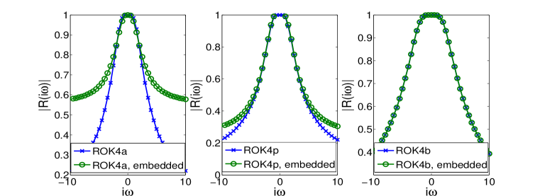
Fig. 4: Stability functions for the main and embedded methods of Rok4a, Rok4p, and Rok4b.

5 Numerical Results

Here we present some results from numerical experiments verifying the properties of the methods discussed above, as well as comparing performance of Rosenbrock-Krylov methods with several standard classical Rosenbrock and Rosenbrock-W methods. Rang3 is a third order Rosenbrock-W method [34], Rodas4 is a fourth order, stiffly accurate classical Rosenbrock method [13, Section IV.10], and Ros4 is a fourth order, L-stable, classical Rosenbrock method [13, Section IV.10].

5.1 Lorenz 96

The nonlinear test is carried out with the Lorenz-96 model [30]. This chaotic model has $N=40$ states, periodic boundary conditions, and is described by the following equations:

(26) $$\frac{dy_{j}}{dt} = -y_{j-1}\;\left(y_{j-2}-y_{j+1}\right)-y_{j}+F\;,\quad j=1,\ldots,N~{},$$

$$y_{-1} = y_{N-1}~{},\quad y_{0}=y_{N}~{},\quad y_{N+1}=y_{1}~{}.$$

The forcing term is $F=8.0$, with $t\in[0,\ 0.3]$.

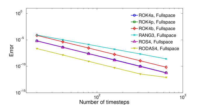
Fig. 5: Precision diagram for Lorenz 96, showing convergence order of methods using a full Jacobian.

	Rang3	Ros4	Rodas4	Rok4a	Rok4p	Rok4b
M = N	2.99	4.01	3.99	4.01	3.99	3.99
M = 4	2.99	3.03	3.05	4.01	3.98	3.99

Table 4: Convergence Rates on Lorenz 96.

Table 4 shows the convergence orders of all methods applied to the Lorenz-96 system, using both the full Jacobian as well as a four dimensional Krylov approximation of the Jacobian. Figure 5 verifies numerically the theoretical order results for all methods using the full Jacobian.

Recall that all methods satisfying the classical Rosenbrock order conditions are also Rosenbrock-K methods of at least order three. Table 4 shows this property, where the third order method Rang3 maintains its order and both fourth order methods, Ros4 and Rodas4, reduce to third order while using the approximate Jacobian.

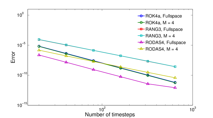
Fig. 6: Precision diagram showing the convergence order of Rok4a, Rang3, and Rodas4 using the full and Krylov approximated Jacobian.

5.2 Dissipative Burger’s equation

We apply the newly derived methods to an ODE system coming from a semi-discretization of a partial differential equation using the method of lines. The dissipative Burger’s equation is a one-dimensional PDE described by

(27) $$\frac{du}{dt}+\frac{d}{dx}\left(\frac{1}{2}u^{2}\right)=\varepsilon\frac{d^{2}u}{dx^{2}},\quad x\in[0,10],\quad t\in[0,\ 0.5],\quad\varepsilon=.001\,,$$

with homogeneous boundary conditions, and initial condition

$$u(x,t=0)=\frac{1}{6}\sin^{2}\,\left(\frac{1}{5}\pi x\right)\,\left(1-x^{2}\right)\,,\quad\varepsilon=.001\,.$$

The spatial discretization is a Nodal Discontinuous Galerkin method using equispaced fourth-order elements, making use of the code base provided for [14].

Figures 7 and 8 show a performance comparison of the newly proposed methods with both Ros4 and Rodas4. The figures show that for problems of even modest size, Rosenbrock-Krylov methods have comparable efficiency with previously existing methods. The increase in relative efficiency between Rosenbrock-K methods and the classical Rosenbrock methods as the problem size increases is a good indicator that Rosenbrock-K methods are likely to be much more efficient than full space methods as problem size increases, and the benefits of solving a reduced system become more pronounced.

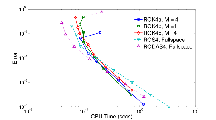
Fig. 7: Precision diagram for Burger’s equation using 10 fourth order elements.

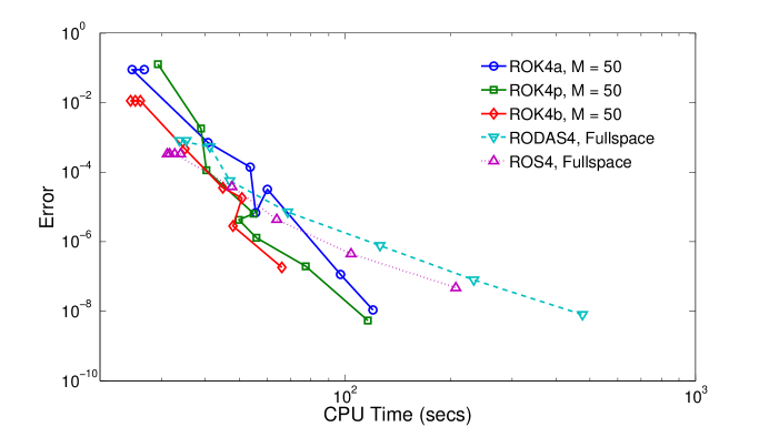
Fig. 8: Precision diagram for Burger’s equation using 400 fourth order elements.

5.3 CBM-IV

Here we give some results for ROK methods applied to a stiff system of ODEs coming from a KPP MATLAB implementation of the CBM-IV model [9]. This problem is based on the Carbon Bond Mechanism IV (CBM-IV), consisting of 32 chemical species involved in 70 thermal and 11 photolytic reactions [37].

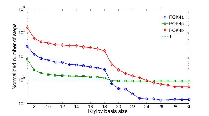
Fig. 9: Number of accepted steps in a full space solution with tolerances of $10^{-2}$ for CBM-IV.

While CBM-IV is a perfect example of a problem for which Rosenbrock-K methods are a poor choice, due to its small size and relatively large number of stiff variables, it does allow us to illustrate numerically the relationship between stability and choice of Krylov basis size. Figure 9 shows the number of timesteps, normalized to a full space solution of the respective method, required to obtain a reasonable solution in a single day simulation of the CBM-IV model. The number of timesteps required for a full space solution are given in Table 5.

$\begin{array}[]{|c|c|c|}\hline\cr\textrm{{\sc Rok4}a}&\textrm{{\sc Rok4}p}&\textrm{{\sc Rok4}b}\\ \hline\cr 1301&10270&261\\ \hline\cr\end{array}$

Table 5: Number of required timesteps in a full space solution with tolerances of $10^{-2}$.

We see from this figure that for small Krylov basis sizes, Rosenbrock-K methods are unstable. However, as the size of the Krylov space nears the size of the full space the behavior of the Rosenbrock-K methods approaches that of the full space method.

5.4 Shallow water equations

We examine the relative performance of the methods on the shallow water equations [29].

(28a) $$\frac{\partial}{\partial t}h+\frac{\partial}{\partial x}(uh)+\frac{\partial}{\partial y}(vh) = 0$$

(28b) $$\frac{\partial}{\partial t}(uh)+\frac{\partial}{\partial x}\left(u^{2}h+\frac{1}{2}gh^{2}\right)+\frac{\partial}{\partial y}(uvh) = 0$$

(28c) $$\frac{\partial}{\partial t}(vh)+\frac{\partial}{\partial x}(uvh)+\frac{\partial}{\partial y}\left(v^{2}h+\frac{1}{2}gh^{2}\right) = 0,$$

with reflective boundary conditions, where $u(x,y,t)$, $v(x,y,t)$ are the flow velocity components and $h(x,y,t)$ is the fluid height. After spatial discretization using centered finite differences on a $32\times 32$ grid the system (28) is brought to the standard ODE form (1) with

$$y=\left[u\,\,v\,\,h\right]^{T}\in\mathbb{R}^{N},\quad f_{y}(t,y)=\mathbf{J}\in\mathbb{R}^{N\times N},~{}~{}N=3072.$$

For all experiments we report only the time discretization errors, calculated against a reference solution computed by MATLAB’s ODE15s solver with absolute and relative tolerances set to $10^{-12}$.

Figure 11 gives an efficiency comparison of the Rosenbrock-K and classical Rosenbrock methods, all methods make use of a sparse Jacobian matrix. This problem illustrates the scalability of the Rosenbrock-K methods, when the stiff subspace of the problem is kept relatively small. Here there are $3072$ state variables, but the Rosenbrock-K methods require only eight basis vectors for stability, and so the cost of computing the Krylov space and solving the small system is much smaller than solving the linear system in the full space.

$\begin{array}[]{|c|c|c|c|}\hline\cr&\textrm{{\sc Rok4}a}&\textrm{{\sc Rok4}p}&\textrm{{\sc Rok4}b}\\ \hline\cr\textrm{Fullspace}&3.85&3.87&3.94\\ \hline\cr\textrm{Exact Jacobian}&3.86&3.88&3.94\\ \hline\cr\textrm{Finite-difference}&3.86&3.88&3.94\\ \hline\cr\textrm{Low accuracy finite-difference}&1.99&0.99&2.01\\ \hline\cr\end{array}$

Table 6: Convergence rates for shallow water equations.

Table 6 shows the convergence rates of the three Rok methods applied with a constant timestep to solve the shallow water problem. We consider the exact Jacobian implementation as well as reduced space approximations of the Jacobian. We compute the Krylov space approximations using exact Jacobian-vector products and using finite difference approximations. In order to assess the impact of the finite difference errors we consider both an accurate implementation of the Jacobian-vector products, where the increment $\delta$ in (19) is carefully chosen, as well as an inaccurate implementation where a large, fixed value of $\delta$ is used.

Fig. 10: Precision diagram for different methods on the shallow water equations problem. The lower order convergence rates are due to the low accuracy finite-difference approximation of Jacobian-vector products.

To verify the results presented in section 3.4 we perform a convergence study for the three Rok methods using a low accuracy finite-difference approximation of the Jacobian-vector products applied to the shallow water equations. Results are presented in Figure 10, The three curves show a distinct change in slope. When the finite-difference error is small compared to the timestep the methods have a convergence orders $3.4$–$3.7$. When the finite-difference error becomes large compared to the timestep Rok4a and Rok4b show second-order and Rok4p shows only first-order. The difference in order when the finite-difference approximation is poor can be explained as follows. Rok4a and Rok4b satisfy the second-order W condition of Figure 1 and have the error term (20) equal nonzero, while Rok4p does not satisfy this additional condition. Rosenbrock-W methods are preferred when finite-differences are the only option for obtaining Jacobian-vector products, and these products cannot be obtained accurately.

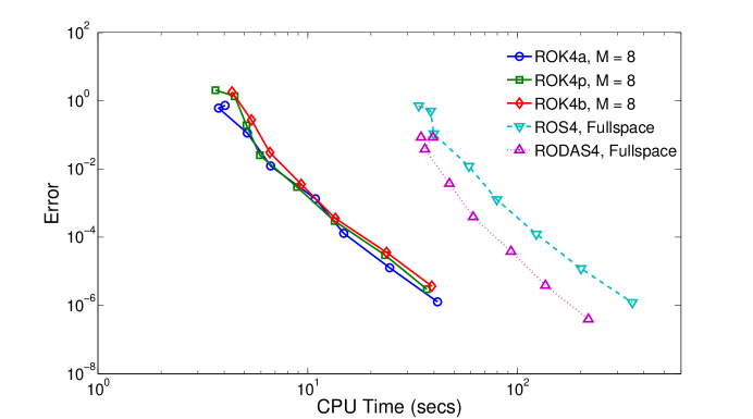
Fig. 11: Precision diagram for the shallow water equations.

With the small basis size requirements in mind we explore in Figure 12 the relative difference in cost, measured by the number of right hand side evaluations, between an explicit Runge-Kutta method and matrix-free Rosenbrock-K methods. Figure 12 shows the number of function evaluations on the $x$-axis and the Error of the resulting solution on the $y$-axis. The number of function evaluations for Rok4a includes those required to compute the matrix-free Jacobian-vector products in the Arnoldi iteration. For the shallow water equations we see that Rosenbrock-K methods perform well against the explicit Runge-Kutta method, when low accuracy is desired and the CFL condition begins to constrain the explicit method.

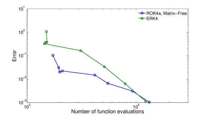
Fig. 12: Comparison of ROKa and ERK4 on the shallow water equations.

6 Conclusions and future work

In this work we have developed a new class of Rosenbrock like integrators, along with a corresponding order condition theory. We consider the ODE integrator and linear solver as a single computational process to develop methods with the least possible amount of implicitness.

The Rosenbrock-K order conditions remove the requirement for accurate solution of the linear systems which constrain the use of approximate methods in classical Rosenbrock integrators. For accuracy of the integration process, the size of the Krylov approximation of the Jacobian need be only as large as the desired order of the method. Stability considerations give stricter requirements on the size of the Krylov basis used, though the exact nature of these requirements is not yet entirely understood and will be the focus of future work. Some numerical investigation, and a result by Wensch [47], give reason to believe that the required size of the Krylov subspace is related to the number of stiff variables in the underlying problem.

The Rosenbrock-K methods developed here have many favorable properties over similar integrators. Rosenbrock-K methods have substantially fewer order conditions than Rosenbrock-W methods, requiring only a single extra order condition for order four methods as opposed to four extra conditions for order three methods in the case of Rosenbrock-W. The reduced number of order conditions allows for methods of higher order, we have given conditions up to order five, or for methods with fewer stages. Further, the structure of Rosenbrock-K methods allows for the computation of a single Krylov subspace at each timestep without the requirement of enriching this space for each internal stage, as is the case for Krylov-ROW methods.

The efficiency of Rosenbrock-K integrators applied to a specific problem is dependent on the stability requirements, and therefore on the stiffness of the underlying problem. We have illustrated this in [43] with the help of a chemical kinetic test problem. For this reason Rosenbrock-K methods are best suited to very large problems in which there is a relatively small number of stiff variables. However, Rosenbrock-K methods are expected to perform at least as well as Krylov-ROW methods in all cases.

References

- [1] M. Botchev, Block Krylov subspace exact time integration of linear ODE systems. part 1: algorithm description. http://arxiv.org/abs/1109.5100, 2011.
- [2] M. Botchev, G. Sleijpen, and H. van der Vors, Low-dimensional Krylov subspace iterations for enhancing stability of time-step integration schemes, tech. rep., University Utrecht, 2001.
- [3] A. Bouhamidi and K. Jbilou, Stein implicit Runge–Kutta methods with high stage order for large-scale ordinary differential equations, Applied Numerical Mathematics, 61 (2011), pp. 149–159.
- [4] P. Brown, H. Walker, R. Wasyk, and C. Woodward, On using approximate finite differences in matrix-free Newton-Krylov methods, SIAM Journal on Numerical Analysis, 46 (2008), pp. 1892–1911.
- [5] P. N. Brown, A. C. Hindmarsh, and L. R. Petzold, Using Krylov methods in the solution of large-scale differential-algebraic systems, SIAM Journal on Scientific Computing, 15 (1994), pp. 1467–1488.
- [6] M. Caliaria and A. Ostermann, Implementation of exponential Rosenbrock-type integrators, Applied Numerical Mathematics, 3–4 (2009), pp. 568–581.
- [7] K. Dekker, Partitioned Krylov subspace iteration in implicit Runge–Kutta methods, Linear Algebra and its Applications, 431 (2009), pp. 488–494.
- [8] K. Evans and D. Knoll, Temporal accuracy analysis of phase change convection simulations using the JFNK-SIMPLE algorithm, International Journal for Numerical Methods in Fluids, 55 (2007).
- [9] M. W. Gery, G. Z. Whitten, J. P. Killus, and M. C. Dodge, A photochemical kinetics mechanism for urban and regional scale computer modeling, Journal of Geophysical Research: Atmospheres, 94 (1989), pp. 12925–12956.
- [10] A. Griewank, Evaluating Derivatives: Principles and Techniques of Algorithmic Differentiation, no. 19 in Frontiers in Appl. Math., SIAM, Philadelphia, PA, 2000.
- [11] I. Grotowskya and J. Ballmanna, Efficient time integration of Navier–Stokes equations, Computers & Fluids, 28 (1996), pp. 243–263.
- [12] E. Hairer, S. Norsett, and G. Wanner, Solving Ordinary Differential Equations I: Nonstiff Problems, Springer, 2008.
- [13] E. Hairer and G. Wanner, Solving Ordinary Differential Equations II: Stiff and Differential-Algebraic Problems, Springer, 2002.
- [14] J. S. Hesthaven and T. Warburton, Nodal Discontinuous Galerkin Methods, Texts in Applied Mathematics, Springer, 2008.
- [15] A. Hindmarsh, LSODKR, stiff ordinary differential equations (ODE) system solver with Krylov iteration with rootfinding, 1991.
- [16] A. Hindmarsh and P. Brown, LSODPK, ordinary differential equations solver for stiff and nonstiff system with Krylov corrector iteration, 1991.
- [17] A. Hindmarsh, P. Brown, and G. Byrne, VODPK: Variable-coefficient ordinary differential equation solver with the Preconditioned Krylov method GMRES for the solution of linear systems. http://www.netlib.org/ode/vodpk.f, 2002.
- [18] M. Hochbruck and C. Lubich, On Krylov subspace approximations to the matrix exponential operator, SIAM Journal on Numerical Analysis, 34 (1997), pp. 1911–1925.
- [19] M. Hochbruck, C. Lubich, and H. Selhofer, Exponential integrators for large systems of differential equations, SIAM Journal of Scientific Computing, 19 (1998), pp. 1552—1574.
- [20] M. Hochbruck and A. Ostermann, Exponential integrators, Acta Numerica, 19 (2012), pp. 209–286.
- [21] M. Hochbruck, A. Ostermann, and J. Schweitzer, Exponential Rosenbrock-type methods, SIAM Journal on Numerical Analysis, 47 (2009), pp. 786–803.
- [22] S. Hosseini and G. Hojjati, Matrix free MEBDF method for the solution of stiff systems of ODEs, Mathematical and Computer Modelling, 29 (1999), pp. 67–77.
- [23] J. Huang, J. Jia, and M. Minion, Accelerating the convergence of spectral deffered correction methods, Journal of Computational Physics, 214 (2006), pp. 633–656.
- [24] J. Huang, J. Jia, and M. Minion, Arbitrary order Krylov deferred correction methods for differential algebraic equations, Journal of Computational Physics, 221 (2007), pp. 739–760.
- [25] J. Huang, J. Jia, and M. Minion, Arbitrary order Krylov deffered corrction methods for differential algebraic equations, Journal of Computational Physics, 221 (2007), pp. 739–760.
- [26] L. Jay, A parallelizable preconditioner for the iterative solution of implicit Runge–Kutta-type methods, Journal of Computational and Applied Mathematics, 111 (1999), pp. 63–76.
- [27] C. Kelley, I. Kevrekidis, and L. Qiao, Newton-Krylov solvers for time-steppers. arXiv:math/0404374v1, 2004.
- [28] D. Knoll and D. Keyes, Jacobian-free Newton–Krylov methods: a survey of approaches and applications, Journal of Computational Physics, 193 (2004), pp. 357–397.
- [29] R. Liska and B. Wendroff, Composite schemes for conservation laws, 1997.
- [30] E. N. Lorenz, Predictability – a problem partly solved, in Predictability of Weather and Climate, Cambridge University Press, 2006.
- [31] C. Lubich and A. Ostermann, Linearly implicit time discretization of nonlinear parabolic equations, IMA Journal on Numerical Mathematics, 15 (1995), pp. 555–583.
- [32] P. Novati, Some secant approximations for Rosenbrock W-methods, Applied Numerical Mathematics, 58 (2008), pp. 195–211.
- [33] H. Podhaisky, R. Weiner, and B. Schmitt, Numerical experiments with Krylov integrators, Applied Numerical Mathematics, 28 (1997), pp. 413–425.
- [34] J. Rang and L. Angermann, New Rosenbrock W-methods of order 3 for partial differential algebraic equations of index 1, BIT Numerical Mathematics, 45 (2005), pp. 761–787.
- [35] R.Weiner, B. Schmitt, and H. Podhaisky, ROWMAP–a ROW-code with Krylov techniques for large stiff ODEs, Applied Numerical Mathematics, 25 (1997), pp. 303–319.
- [36] Y. Saad, Iterative methods for sparse linear systems, PWS Pub. Co., Boston, 1996.
- [37] A. Sandu, J. Verwer, M. V. Loon, G. Carmichael, F. Potra, D. Dabdub, and J. Seinfeld, Benchmarking stiff ode solvers for atmospheric chemistry problems-i. implicit vs explicit, Atmospheric Environment, 31 (1997), pp. 3151 – 3166. ¡ce:title¿EUMAC: European Modelling of Atmospheric Constituents.
- [38] B. Schmitt and R. Weiner, Matrix free W-methods using a multiple Arnoldi iteration, Applied Numerical Mathematics, 18 (1995), pp. 307–320.
- [39] , Polynomial preconditioning in Krylov-ROW-methods, Applied Numerical Mathematics, 28 (1998), pp. 427–437.
- [40] J. C. Schulze, P. J. Schmid, and J. L. Sesterhenn, Exponential time integration using Krylov subspaces, International Journal for Numerical Methods in Fluids, 60 (2008), pp. 561–609.
- [41] K. Strehmel, R. Weiner, and M. Büttner, Order results for Rosenbrock type methods on classes of stiff equations, Numerische Mathematik, 59 (1991), pp. 723–737.
- [42] M. Tokman, Efficient integration of large stiff systems of ODEs with exponential propagation iterative (EPI) methods, Journal of Computational Physics, 213 (2006), pp. 748–776.
- [43] P. Tranquilli and A. Sandu, Rosenbrock-Krylov methods for large systems of differential equations, ArXiv e-prints, (2013).
- [44] H. A. van der Vorst, Iterative Methods for Large Linear Systems, Cambridge University Press, 2003.
- [45] R. Weiner and B. Schmitt, Consistency of Krylov-W-methods in initial value problems, Tech. Rep. 14, Fachbereich Mathematik und Informatik, Martin-Luther-Universitat Halle-Wittenberg, 1995.
- [46] , Order results for Krylov-W methods, Computing, 61 (1998), pp. 69–89.
- [47] J. Wensch, Krylov-ROW methods for DAEs of index 1 with applications to viscoelasticity, Applied Numerical Mathematics, 53 (2005), pp. 527–541.