Introduction to
Judea Pearl’s Do-Calculus

Abstract

This is a purely pedagogical paper with no new results. The goal of the paper is to give a fairly self-contained introduction to Judea Pearl’s do-calculus, including proofs of his 3 rules.

1 Introduction

Judea Pearl’s do-calculus is a part of his theory of probabilistic causality, which itself is a part of the study of Bayesian networks (for which he is largely responsible too). For a good textbook on Bayesian Networks, see, for example, Ref.[1] by Koller and Friedman.

The goal of this paper is to give a fairly self-contained introduction to Judea Pearl’s do-calculus. Pearl first enunciated his calculus in the 1995 paper Ref.[2]. Our paper is mostly based on Ref.[2]. Compared with Ref.[2], the scope of our paper is smaller (for example, we don’t discuss “identifiability” at all). However, for the material we do cover, we present some extra details which are not found in Ref.[2] and which might be helpful to beginners. Ref.[2] is a wonderful paper and we fully expect our readers to read it at the same time that they read this one. We just think that it might help the readers of Ref.[2] to hear the same thing explained by someone else, in slightly different words, and from a slightly different perspective.

In this paper, we give full proofs of the 3 rules of do-calculus. Our proofs are almost the same but slightly different from those found in the Appendix of Ref.[2].

Since 1995, some interesting new consequences, ramifications and applications of Pearl’s do-calculus have been found. These were reviewed recently (2012) by Pearl in Ref.[3].

2 Basic Notation

In this section, we will define some basic notation that will be used later in the paper.

We will use $\delta_{a}^{b}$ or $\delta(a,b)$ to denote the Kronecker delta function (equals 1 if $a=b$ and 0 otherwise).

We will indicate random variables by underlined symbols and indicate their possible values (a.k.a. states, instances) by the same letter, but not underlined. For example, ${\,\underline{a}\,}$ takes on values $a$. Many people, Pearl and coworkers included, indicate random variables by capital letters and their possible values by lower case letters. For example, $A$ takes on values $a$.

Given a probability distribution $P_{{\,\underline{a}\,},{\,\underline{b}\,}}(a,b)$, let

$$P(a:b)=\frac{P(a,b)}{P(a)P(b)}=\frac{P(a|b)}{P(a)}\;,$$ (1)

and

$$P(a:b|c)=\frac{P(a,b|c)}{P(a|c)P(b|c)}=\frac{P(a|b,c)}{P(a|c)}\;.$$ (2)

We will indicate n-tuples (vectors, ordered sets) by a letter followed by a dot, as in $x.=(x_{1},x_{2},\ldots,x_{n})$. The dot is intended to suggest that the subscript is free. Many people denote n-tuples by putting an arrow over the letter (as in $\vec{x}$) or by using a boldface letter (an in $\bf{x}$).

Often, we will treat two n-tuples of random variables as if they were plain sets and use them in conjunction with standard set symbols such as those for subset, union, intersection and subtraction. For example, if ${\,\underline{x}\,}.$ and ${\,\underline{y}\,}.$ are an n-tuple and an m-tuple, respectively, where $m$ and $n$ are not necessarily the same, then we might write ${\,\underline{x}\,}.\subset{\,\underline{y}\,}.$, ${\,\underline{x}\,}.\cup{\,\underline{y}\,}.$, ${\,\underline{x}\,}.\cap{\,\underline{y}\,}.$ and ${\,\underline{x}\,}.-{\,\underline{y}\,}.$. In such contexts, we will sometimes not distinguish between ${\,\underline{x}\,}_{j}$ and the singleton set $\{{\,\underline{x}\,}_{j}\}$. For example we might write ${\,\underline{x}\,}.-{\,\underline{x}\,}_{j}$ instead of ${\,\underline{x}\,}.-\{{\,\underline{x}\,}_{j}\}$.

A classical Bayesian network is a DAG (directed acyclic graph) where each vertex (a.k.a. node) is labeled by a random variable ${\,\underline{x}\,}_{j}$ and is assigned a transition probability matrix about which we will say more below. Let ${\,\underline{x}\,}.=({\,\underline{x}\,}_{1},{\,\underline{x}\,}_{2},\ldots,{\,\underline{x}\,}_{N})$. Arrows are also called directed edges. Each node ${\,\underline{v}\,}$ with an arrow going from ${\,\underline{v}\,}$ to ${\,\underline{x}\,}_{j}$ is called a parent of ${\,\underline{x}\,}_{j}$ and the set of such parent nodes is denoted by ${\,\underline{pa}\,}({\,\underline{x}\,}_{j})$. Each node ${\,\underline{v}\,}$ with an arrow going from ${\,\underline{x}\,}_{j}$ to ${\,\underline{v}\,}$ is called a child of ${\,\underline{x}\,}_{j}$ and the set of such children nodes is denoted by ${\,\underline{ch}\,}({\,\underline{x}\,}_{j})$. Each node ${\,\underline{x}\,}_{j}$ is assigned a transition probability matrix $P(x_{j}|pa({\,\underline{x}\,}_{j}))$ that depends on the value $x_{j}$ of node ${\,\underline{x}\,}_{j}$ and the values $pa({\,\underline{x}\,}_{j})$ of nodes ${\,\underline{pa}\,}({\,\underline{x}\,}_{j})$. The entire Bayesian network is assigned a total probability

$$P(x.)=\prod_{j=1}^{N}P(x_{j}|pa({\,\underline{x}\,}_{j}))\;.$$ (3)

3 Subgraphs and Augmented Graphs

In this section, we will define certain subgraphs and augmented graphs, derived from a graph $G$, that will be especially useful to us later on.

Suppose that graph $G$ has nodes ${\,\underline{x}\,}.$ and ${\,\underline{a}\,}.\subset{\,\underline{x}\,}.$.

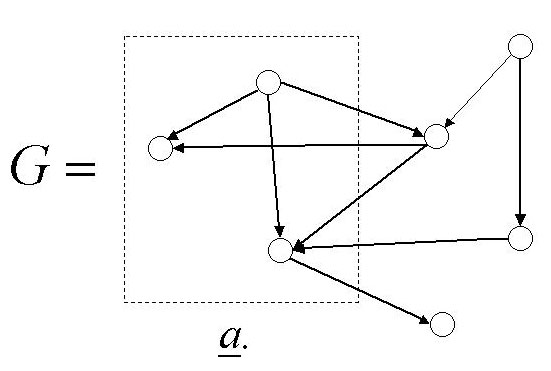
Figure 1: A corral for subset ${\,\underline{a}\,}.$ of the nodes ${\,\underline{x}\,}.$ of graph $G$.

We can draw a frame that encloses the nodes ${\,\underline{a}\,}.$ and leaves the nodes ${\,\underline{x}\,}.-{\,\underline{a}\,}.$ outside. We will refer to such an enclosure as the ${\,\underline{a}\,}.$ “corral” (See Fig.1 for an example).

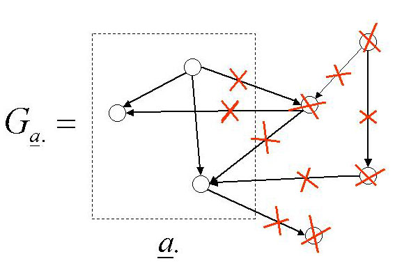
Figure 2: Graph $G_{{\,\underline{a}\,}.}$ arises from graph $G$ of Fig.1 if we restrict $G$ to node set ${\,\underline{a}\,}.$. Arrows or nodes with a red cross through them should be erased.

We will use $G_{{\,\underline{a}\,}.}$ to denote the “restriction” of graph $G$ wherein nodes ${\,\underline{x}\,}.-{\,\underline{a}\,}.$ and any arrows connected to ${\,\underline{x}\,}.-{\,\underline{a}\,}.$ have been erased. (See Fig.2 for an example).

Figure 3: Graph $G_{{\stackrel{{\scriptstyle\wedge}}{{{\,\underline{a}\,}}}}.}$ arises from graph $G$ of Fig.1 if we erase from $G$ all arrows entering node set ${\,\underline{a}\,}.$. Arrows or nodes with a red cross through them should be erased.

We will use $G_{{\stackrel{{\scriptstyle\wedge}}{{{\,\underline{a}\,}}}}.}$ to denote the graph $G$ with arrows entering ${\,\underline{a}\,}.$ erased. Mnemonic: Think of the “hat” on top of ${\,\underline{a}\,}.$ as being the arrow-head of an arrow exiting ${\,\underline{a}\,}.$. Only arrows of this type (that is, those that are exiting ${\,\underline{a}\,}.$) are allowed.(See Fig.3 for an example).

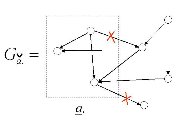
Figure 4: Graph $G_{{\stackrel{{\scriptstyle\vee}}{{{\,\underline{a}\,}}}}.}$ arises from graph $G$ of Fig.1 if we erase from $G$ all arrows exiting node set ${\,\underline{a}\,}.$. Arrows or nodes with a red cross through them should be erased.

We will use $G_{{\stackrel{{\scriptstyle\vee}}{{{\,\underline{a}\,}}}}.}$ to denote the graph $G$ with arrows exiting ${\,\underline{a}\,}.$ erased. Mnemonic: Think of the “vee” on top of ${\,\underline{a}\,}.$ as being the arrow-head of an arrow entering ${\,\underline{a}\,}.$. Only arrows of this type (that is, those that are entering ${\,\underline{a}\,}.$) are allowed.(See Fig.4 for an example).

We will use $G\leftarrow{\,\underline{rt}\,}({\,\underline{a}\,}.)$ to denote the augmented graph obtained by adding to graph $G$ a node set ${\,\underline{rt}\,}({\,\underline{a}\,}.)$ and arrows from ${\,\underline{rt}\,}({\,\underline{a}\,}.)$ to node set ${\,\underline{a}\,}.$ (${\,\underline{a}\,}.$ is contained in $G$). For each ${\,\underline{a}\,}_{j}\in{\,\underline{a}\,}.$, one adds exactly one twin node ${\,\underline{rt}\,}({\,\underline{a}\,}_{j})\in{\,\underline{rt}\,}({\,\underline{a}\,}.)$, and one arrow from the “root” node ${\,\underline{rt}\,}({\,\underline{a}\,}_{j})$ to ${\,\underline{a}\,}_{j}$.(See Fig.5 for an example).

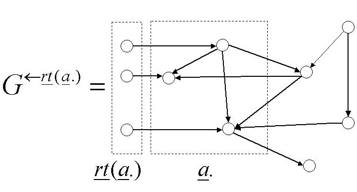
Figure 5: Graph $G\leftarrow{\,\underline{rt}\,}({\,\underline{a}\,}.)$ arises from graph $G$ of Fig.1 if add to $G$ a node set ${\,\underline{rt}\,}({\,\underline{a}\,}.)$ of root nodes for ${\,\underline{a}\,}.$.

One can describe a set or family of graphs by using what I call a graph template. In a graph template, some corrals have bans or restrictions on the types of arrows that are allowed to cross the fence. A ban is represented by an arrow with a red cross on it to indicate the type of arrow that is forbidden. One can ban this way either all arrows entering the corral or all arrows exiting the corral or all arrows going from one corral to another. In other words, if nodes are like cows, some corrals have one way gates that ban certain types of bovine movement. See Fig.6 for an example of a graph template $TG$.

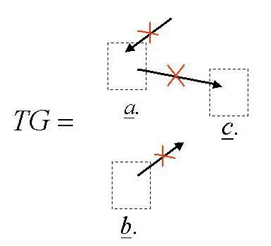
Figure 6: Example of a graph template $TG$. This one has a ban on arrows entering ${\,\underline{a}\,}.$, a ban on arrows exiting ${\,\underline{b}\,}.$, and a ban on arrows going from ${\,\underline{a}\,}.$ to ${\,\underline{c}\,}.$.

For $f\in\{ch,de,pa,an\}$ and ${\,\underline{v}\,}.\subset{\,\underline{x}\,}$, let $f({\,\underline{a}\,}.,G_{{\,\underline{v}\,}.})$ be the set of nodes which are the children, descendants, parents and ancestors, respectively, of ${\,\underline{a}\,}.$ in the graph $G_{{\,\underline{v}\,}.}$. We will write $f({\,\underline{a}\,}.)$ instead of $f({\,\underline{a}\,}.,G_{{\,\underline{v}\,}.})$ when $G_{{\,\underline{v}\,}.}=G_{{\,\underline{x}\,}.}=G$. If $f^{(n)}(\cdot)$ indicates application $n$ times of the function $f(\cdot)$, then $de({\,\underline{a}\,}.,G_{{\,\underline{v}\,}.})=\cup_{n=1}^{\infty}ch^{(n)}({\,\underline{a}\,}.,G_{{\,\underline{v}\,}.})$ and $an({\,\underline{a}\,}.,G_{{\,\underline{v}\,}.})=\cup_{n=1}^{\infty}pa^{(n)}({\,\underline{a}\,}.,G_{{\,\underline{v}\,}.})$. For $f\in\{ch,de,pa,an\}$, let $\overline{f}({\,\underline{a}\,}.,G_{{\,\underline{v}\,}.})=f({\,\underline{a}\,}.,G_{{\,\underline{v}\,}.})\cup{\,\underline{a}\,}.$ and call $\overline{f}(\cdot)$ the closure of $f(\cdot)$.

4 D-Separation

In this section, we will explain the d-sep (dependence separation) theorem, which tells us how to diagnose from a graph $G$ whether ${\,\underline{a}\,}.$ and ${\,\underline{b}\,}.$ are probabilistically conditionally independent at fixed ${\,\underline{e}\,}.$, where ${\,\underline{a}\,}.,{\,\underline{b}\,}.,{\,\underline{e}\,}.$ are disjoint subsets of nodes of $G$.

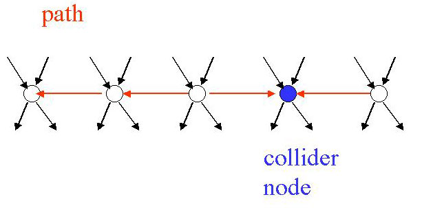
Figure 7: A typical path of a graph and a typical collider node in that path.

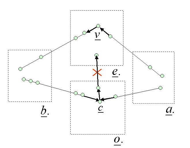
Figure 8: Two types of paths from ${\,\underline{a}\,}.$ to ${\,\underline{b}\,}.$ that are blocked at fixed ${\,\underline{e}\,}.$. The set ${\,\underline{o}\,}.$ is defined to contain all “other” nodes; i.e., all nodes not in ${\,\underline{a}\,}.\cup{\,\underline{b}\,}.\cup{\,\underline{e}\,}.$. Note that the collider node ${\,\underline{c}\,}$ can have descendants in either ${\,\underline{b}\,}.,{\,\underline{o}\,}.$ or ${\,\underline{a}\,}.$. Note also that even though in this figure we put ${\,\underline{c}\,}$ in the ${\,\underline{o}\,}.$ corral, it could also be in ${\,\underline{b}\,}.$ or ${\,\underline{a}\,}.$.

Suppose that graph $G$ has nodes ${\,\underline{x}\,}.$ and ${\,\underline{a}\,}.\subset{\,\underline{x}\,}.$. If all the nodes in ${\,\underline{a}\,}.$ are like the beads in a beaded string with one arrow between adjacent beads, where the direction of the arrows may change inside the string, then we will call ${\,\underline{a}\,}.$ an undirected path of $G$.

We will use $Path_{G}({\,\underline{A}\,}<{\,\underline{B}\,})$ to denote the set of all undirected paths in graph $G$ that start at node ${\,\underline{A}\,}$ and end at node ${\,\underline{B}\,}$. Here $<$ means that there are $\geq 1$ arrows (in whatever direction) and $\geq 0$ nodes between ${\,\underline{A}\,}$ and ${\,\underline{B}\,}$. We will also use ${\,\underline{A}\,}\leq{\,\underline{B}\,}$ if ${\,\underline{A}\,}$ and ${\,\underline{B}\,}$ could be the same node. We will also write a comma instead of a $<$ between the ${\,\underline{A}\,}$ and ${\,\underline{B}\,}$ if there is only one arrow between ${\,\underline{A}\,}$ and ${\,\underline{B}\,}$. If ${\,\underline{a}\,}.$ and ${\,\underline{b}\,}.$ are disjoint subsets of ${\,\underline{x}\,}.$, let $Path_{G}({\,\underline{a}\,}.<{\,\underline{b}\,}.)=\cup_{{\,\underline{A}\,}\in{\,\underline{a}\,}.,{\,\underline{B}\,}\in{\,\underline{b}\,}.}Path({\,\underline{A}\,}<{\,\underline{B}\,})$. If ${\,\underline{a}\,}.^{(1)},{\,\underline{a}\,}.^{(2)},\ldots,{\,\underline{a}\,}.^{(n)}$ are disjoint subsets of ${\,\underline{x}\,}.$, define $Path_{G}({\,\underline{a}\,}.^{(1)}<{\,\underline{a}\,}.^{(2)}<\ldots<{\,\underline{a}\,}.^{(n)})$ as the obvious generalization of this notation.

Given an undirected path $\gamma$ of $G$, any node which has arrows impinging upon it from both sides of the string will be called a collider node of $\gamma$. (See Fig.7 for an example). We will denote the set of all collider nodes of path $\gamma$ by $col(\gamma)$.

Suppose a graph $G$ has nodes ${\,\underline{x}\,}.$ and that ${\,\underline{x}\,}.$ equals the union of the disjoint sets ${\,\underline{a}\,},{\,\underline{b}\,}.,{\,\underline{e}\,}.,$ and ${\,\underline{o}\,}.$. $\gamma\in Path({\,\underline{a}\,}.<{\,\underline{b}\,}.)$ is said to be blocked at fixed ${\,\underline{e}\,}.$ if either

• $(\exists{\,\underline{v}\,}\in\gamma)[{\,\underline{v}\,}\notin col(\gamma)\mbox{ and }{\,\underline{v}\,}\in{\,\underline{e}\,}.$], or

• $(\exists{\,\underline{c}\,}\in\gamma)[{\,\underline{c}\,}\in col(\gamma)\mbox{ and }\overline{de}({\,\underline{c}\,})\cap{\,\underline{e}\,}.=\emptyset]$.

  See Fig.4 for a picture of these two types of blocked paths. I like to think of the non-collider node ${\,\underline{v}\,}$ as a canyon pass which is blocked by an obstacle (like a boulder) in ${\,\underline{e}\,}.$ thus impeding information and cattle from flowing through the path. As for the collider node ${\,\underline{c}\,}$, I like to think of it as a deep sink-hole that is an obstacle to cattle. However, if sink-hole ${\,\underline{c}\,}$ is in ${\,\underline{e}\,}.$ or even if merely one of its descendants is in ${\,\underline{e}\,}.$, then this has the effect of filling that sink-hole so that information and cattle can once again flow through the path.

By negating the previous definition, we immediately get that $\gamma\in Path({\,\underline{a}\,}.<{\,\underline{b}\,}.)$ is unblocked at fixed ${\,\underline{e}\,}.$ if

• $(\forall{\,\underline{v}\,}\in\gamma)[{\,\underline{v}\,}\notin col(\gamma)\implies{\,\underline{v}\,}\notin{\,\underline{e}\,}.]$, and

• $(\forall{\,\underline{c}\,}\in\gamma)[{\,\underline{c}\,}\in col(\gamma)\implies\overline{de}({\,\underline{c}\,})\cap{\,\underline{e}\,}.\neq\emptyset]$.

We write $({\,\underline{a}\,}.\bot{\,\underline{b}\,}.|{\,\underline{e}\,}.)_{G}$ and read this as ${\,\underline{a}\,}.$ and ${\,\underline{b}\,}.$ are d-sep (dependance-separated) at fixed ${\,\underline{e}\,}.$ in graph $G$ if all $\gamma\in Path_{G}({\,\underline{a}\,}.<{\,\underline{b}\,}.)$ are blocked at fixed ${\,\underline{e}\,}.$.

Claim 1

(D-Sep Theorem):
$({\,\underline{a}\,}.\bot{\,\underline{b}\,}.|{\,\underline{e}\,}.)_{G}$ if and only if, for all possible values of $a.,b.,e.$, $P_{G}(a.:b.|e.)=1$, or, equivalently, $P_{G}(a.|b.,e.)=P_{G}(a.|e.)$.

proof: See Ref.[2] for a history of this theorem, including pertinent references. Ref.[2] also describes and gives references for an alternative graphical method, invented by Lauritzen, of diagnosing d-sep.
QED

5 Uprooting And Mowing a Node

In this section, we will define two operations for pruning the arrows connected to a node. One operation “uproots the node”, meaning that it erases all the roots (i.e., incoming arrows) of the node. The other “mows the node”, meaning that it erases all the stems (i.e., outgoing arrows) of the node. Uprooting a node is called an “intervention” by Pearl and co-workers.

Through out this section, let $G$ be a graph with nodes ${\,\underline{x}\,}.$ and let ${\,\underline{a}\,}.,{\,\underline{b}\,}.,{\,\underline{e}\,}.$ be 3 disjoints subsets of ${\,\underline{x}\,}.$.

5.1 Definitions

• Uprooting

  We define as follows the probability that ${\,\underline{b}\,}.=b.$ when ${\,\underline{a}\,}.=a.$ is uprooted:

  $$P(b.|{\stackrel{{\scriptstyle\wedge}}{{a}}}.)=\frac{P_{G_{{\stackrel{{\scriptstyle\wedge}}{{{\,\underline{a}\,}}}}.}}(a.,b.)}{P_{G_{{\stackrel{{\scriptstyle\wedge}}{{{\,\underline{a}\,}}}}.}}(a.)}\neq P_{G}(b.|a.)\;.$$ (4)

  Here $P_{G_{{\stackrel{{\scriptstyle\wedge}}{{{\,\underline{a}\,}}}}.}}(x.)$ is the probability distribution for the subgraph $G_{{\stackrel{{\scriptstyle\wedge}}{{{\,\underline{a}\,}}}}.}$ of $G$. $P_{G_{{\stackrel{{\scriptstyle\wedge}}{{{\,\underline{a}\,}}}}.}}(x.)$ is defined from $P(x.)$ by replacing $P(a_{j}|pa({\,\underline{a}\,}_{j}))$ by $P(a_{j})$ for all $j$. Note that when we do this replacement, all the arrows entering ${\,\underline{a}\,}.$ (the “roots” of ${\,\underline{a}\,}.$) are being erased or “severed”.

  Other notations used in the literature for $P(b.|{\stackrel{{\scriptstyle\wedge}}{{a}}}.)$ are $P(b.|do({\,\underline{a}\,}.)=a.)$ (where $do(\cdot)$ is called the do operator), and $P_{a.}(b.)$. We will sometimes write $[{\cal S}]^{\wedge}$ instead of ${\stackrel{{\scriptstyle\wedge}}{{{\cal S}}}}$, especially when ${\cal S}$ is a long expression.

  An equivalent definition of $P(b.|{\stackrel{{\scriptstyle\wedge}}{{a}}}.)$ is as follows. We define

  $$P(x.-a.|{\stackrel{{\scriptstyle\wedge}}{{a}}}.) = \frac{P(x.)}{\prod_{j:{\,\underline{x}\,}_{j}\in{\,\underline{a}\,}.}P(x_{j}|pa({\,\underline{x}\,}_{j}))}$$ (5a)

  $$= \prod_{j:{\,\underline{x}\,}_{j}\in({\,\underline{x}\,}.-{\,\underline{a}\,}.)}P(x_{j}|pa({\,\underline{x}\,}_{j}))\;.$$ (5b)

  Note that $\sum_{x.-a.}P(x.-a.|{\stackrel{{\scriptstyle\wedge}}{{a}}}.)=1$. Note also that if ${\,\underline{a}\,}.=({\,\underline{a}\,}_{1},{\,\underline{a}\,}_{2},\ldots,{\,\underline{a}\,}_{n})$, then $P(x.-a.|{\stackrel{{\scriptstyle\wedge}}{{a}}}.)=P(x.-a.|{\stackrel{{\scriptstyle\wedge}}{{a}}}_{1},{\stackrel{{\scriptstyle\wedge}}{{a}}}_{2},\ldots,{\stackrel{{\scriptstyle\wedge}}{{a}}}_{n})$.

  Next we define

  $$P(b.|{\stackrel{{\scriptstyle\wedge}}{{a}}}.)=\sum_{x.-(b.\cup a.)}P(x.-a.|{\stackrel{{\scriptstyle\wedge}}{{a}}}.)\;.$$ (6)

  We also define

  $$P(b.|{\stackrel{{\scriptstyle\wedge}}{{a}}}.,e.)=\frac{P(b.,e.|{\stackrel{{\scriptstyle\wedge}}{{a}}}.)}{P(e.|{\stackrel{{\scriptstyle\wedge}}{{a}}}.)}\;.$$ (7)

  I like to call $P(b.|{\stackrel{{\scriptstyle\wedge}}{{a}}}.,e.)$ the probability of ${\,\underline{b}\,}.$ conditioned on ${\,\underline{e}\,}.$, and with ${\,\underline{a}\,}.$ uprooted.

  Yet another equivalent definition of $P(b.|{\stackrel{{\scriptstyle\wedge}}{{a}}}.)$ is as follows. For this definition, we begin by augmenting the graph $G$ to $G\leftarrow{\,\underline{rt}\,}({\,\underline{a}\,}.)$. In the new graph, each node ${\,\underline{a}\,}_{j}$ has a new incoming arrow. We define the transition matrices for the nodes ${\,\underline{a}\,}_{j}$ in the new graph from the transition matrices of the old graph as follows. For all $j$ and for all values $a_{j}$ of ${\,\underline{a}\,}_{j}$, let

  $$P(a_{j}|pa({\,\underline{a}\,}_{j},G),rt({\,\underline{a}\,}_{j}))=P(a_{j})\delta_{rt({\,\underline{a}\,}_{j})}^{1}+P(a_{j}|pa({\,\underline{a}\,}_{j},G))\delta_{rt({\,\underline{a}\,}_{j})}^{0}\;.$$ (8)

  Note that

  $$\left\{\begin{array}[]{l}P(b.|a.,rt({\,\underline{a}\,}.)=0)=P(b.|a.)\\ P(b.|a.,rt({\,\underline{a}\,}.)=1)=P(b.|{\stackrel{{\scriptstyle\wedge}}{{a}}}.)\end{array}\right.\;,$$ (9)

  where $rt({\,\underline{a}\,}.)=n$ for $n\in\{0,1\}$ means $rt({\,\underline{a}\,}_{j})=n$ for all $j$. Thus, node set ${\,\underline{rt}\,}({\,\underline{a}\,}.)$ acts like a switch. When it is on (i.e., when it equals 1), all the roots of node set ${\,\underline{a}\,}.$ are severed.

• Mowing

  Note that

  $$P(x.) = \prod_{j}P(x_{j}|pa({\,\underline{x}\,}_{j}))$$ (10a)

  $$= \prod_{j:{\,\underline{x}\,}_{j}\in({\,\underline{x}\,}.-{\,\underline{a}\,}.)}\left\{P(x_{j}|pa({\,\underline{x}\,}_{j}))\right\}\prod_{j:{\,\underline{x}\,}_{j}\in{\,\underline{a}\,}.}\left\{P(x_{j}|pa({\,\underline{x}\,}_{j}))\right\}$$ (10b)

  $$= P(x.-a.|[a.]^{\wedge})P(a.|[x.-a.]^{\wedge})\;.$$ (10c)

  We define as follows the probability that ${\,\underline{x}\,}.=x.$ when ${\,\underline{a}\,}.={a^{\prime}_{.}}$ is mowed:

  $$P_{{\stackrel{{\scriptstyle\vee}}{{{\,\underline{a}\,}}}}.({a^{\prime}_{.}})}(x.) = \left[P(x.-a.|[a.]^{\wedge})\right]_{a.\rightarrow{a^{\prime}_{.}}}P(a.|[x.-a.]^{\wedge})$$ (11a)

  $$= P(x.-a.|[{a^{\prime}_{.}}]^{\wedge})P(a.|[x.-a.]^{\wedge})\;.$$ (11b)

  Note that we set to ${a^{\prime}_{.}}$ the value of ${\,\underline{a}\,}.$ at the destinations of the arrows exiting ${\,\underline{a}\,}.$. By doing this, we are severing the outgoing arrows of ${\,\underline{a}\,}.$. Note that $\sum_{x.}P_{{\stackrel{{\scriptstyle\vee}}{{{\,\underline{a}\,}}}}.({a^{\prime}_{.}})}(x.)=1$ and $P_{{\stackrel{{\scriptstyle\vee}}{{{\,\underline{a}\,}}}}.({a^{\prime}_{.}})}(x.)=P_{\prod_{j}{\stackrel{{\scriptstyle\vee}}{{{\,\underline{a}\,}}}}_{j}(a_{j}^{\prime})}(x.)$.

  Next we define

  $$P_{{\stackrel{{\scriptstyle\vee}}{{{\,\underline{a}\,}}}}.({a^{\prime}_{.}})}(a.,b.)\sum_{x.-(a.\cup b.)}P_{{\stackrel{{\scriptstyle\vee}}{{{\,\underline{a}\,}}}}.({a^{\prime}_{.}})}(x.)\;.$$ (12)

  We also define

  $$P_{{\stackrel{{\scriptstyle\vee}}{{{\,\underline{a}\,}}}}.({a^{\prime}_{.}})}(b.|a.,e.)=\frac{P_{{\stackrel{{\scriptstyle\vee}}{{{\,\underline{a}\,}}}}.({a^{\prime}_{.}})}(a.,b.,e.)}{P_{{\stackrel{{\scriptstyle\vee}}{{{\,\underline{a}\,}}}}.({a^{\prime}_{.}})}(a.,e.)}\;.$$ (13)

  Note that summing both sides of Eq.(11b) over $a.$ yields

  $$P_{{\stackrel{{\scriptstyle\vee}}{{{\,\underline{a}\,}}}}.({a^{\prime}_{.}})}(x.-a.)=P(x.-a.|[{a^{\prime}_{.}}]^{\wedge})\;,$$ (14)

  and summing both sides of Eq.(14) over $x.-(a.\cup b.)$ yields

  $$P_{{\stackrel{{\scriptstyle\vee}}{{{\,\underline{a}\,}}}}.({a^{\prime}_{.}})}(b.)=P(b.|[{a^{\prime}_{.}}]^{\wedge})\;.$$ (15)

5.2 Operators

Let $pd({\,\underline{x}\,}.)$ be the set of all possible probability distributions for ${\,\underline{x}\,}.$, where ${\,\underline{x}\,}.$ labels the nodes of the graph $G$. Let ${\cal L}(pd({\,\underline{x}\,}.))$ denote the set of all linear combinations over the reals of the elements of $pd({\,\underline{x}\,}.)$. It is convenient to define linear operators acting on ${\cal L}(pd({\,\underline{x}\,}.))$ whose effect is to mow and uproot a node.

Let

$$Cond_{{\,\underline{a}\,}.}P(a.,b.)=P(b.|a.)\;.$$ (16)

• Uprooting

  We define as follows a linear operator $\delta_{{\stackrel{{\scriptstyle\wedge}}{{{\,\underline{a}\,}}}}.}$ that does uprooting of ${\,\underline{a}\,}.$

  $$\delta_{{\stackrel{{\scriptstyle\wedge}}{{{\,\underline{a}\,}}}}.}P(a.,b.)=P(b.|{\stackrel{{\scriptstyle\wedge}}{{a}}}.)\;.$$ (17)

  Note that $\delta_{{\stackrel{{\scriptstyle\wedge}}{{{\,\underline{a}\,}}}}.}=\prod_{j}\delta_{{\stackrel{{\scriptstyle\wedge}}{{{\,\underline{a}\,}}}}_{j}}$ and $\delta_{{\stackrel{{\scriptstyle\wedge}}{{{\,\underline{a}\,}}}}.}P(a.)=1$. Next we extend the domain of $\delta_{{\stackrel{{\scriptstyle\wedge}}{{{\,\underline{a}\,}}}}.}$ as follows so that, besides acting on ${\cal L}(pd({\,\underline{x}\,}.))$, it can also act on a ratio of two elements of ${\cal L}(pd({\,\underline{x}\,}.))$.

  $$\delta_{{\stackrel{{\scriptstyle\wedge}}{{{\,\underline{a}\,}}}}.}P(b.|a.,e.)=\frac{\delta_{{\stackrel{{\scriptstyle\wedge}}{{{\,\underline{a}\,}}}}.}P(a.,b.,e.)}{\delta_{{\stackrel{{\scriptstyle\wedge}}{{{\,\underline{a}\,}}}}.}P(a.,e.)}\;.$$ (18)

  Claim 2

  $$\delta_{{\stackrel{{\scriptstyle\wedge}}{{{\,\underline{a}\,}}}}.}P(a.,b.)=P(b.|{\stackrel{{\scriptstyle\wedge}}{{a}}}.)\;,$$ (19)

  $$\delta_{{\stackrel{{\scriptstyle\wedge}}{{{\,\underline{a}\,}}}}.}P(b.)=\sum_{a.}P(b.|{\stackrel{{\scriptstyle\wedge}}{{a}}}.)\;,\;\;\left[\delta_{{\stackrel{{\scriptstyle\wedge}}{{{\,\underline{a}\,}}}}.}\sum_{a.}=\sum_{a.}\delta_{{\stackrel{{\scriptstyle\wedge}}{{{\,\underline{a}\,}}}}.}\right]\;,$$ (20)

  $$\delta_{{\stackrel{{\scriptstyle\wedge}}{{{\,\underline{a}\,}}}}.}P(b.|a.)=P(b.|{\stackrel{{\scriptstyle\wedge}}{{a}}}.)\;,\;\;\left[\delta_{{\stackrel{{\scriptstyle\wedge}}{{{\,\underline{a}\,}}}}.}Cond_{{\,\underline{a}\,}.}=\delta_{{\stackrel{{\scriptstyle\wedge}}{{{\,\underline{a}\,}}}}.}\right]\;.$$ (21)

  proof: This all follows easily from the linearity of $\delta_{{\stackrel{{\scriptstyle\wedge}}{{{\,\underline{a}\,}}}}.}$ and Eqs.(17) and (18).
  QED

• Mowing

  We define as follows a linear operator $\delta_{{\stackrel{{\scriptstyle\vee}}{{{\,\underline{a}\,}}}}.({a^{\prime}_{.}})}$ that does mowing of ${\,\underline{a}\,}.$ to ${a^{\prime}_{.}}$

  $$\delta_{{\stackrel{{\scriptstyle\vee}}{{{\,\underline{a}\,}}}}.({a^{\prime}_{.}})}P(a.,b.)=P_{{\stackrel{{\scriptstyle\vee}}{{{\,\underline{a}\,}}}}.({a^{\prime}_{.}})}(a.,b.)\;.$$ (22)

  Note that $\delta_{{\stackrel{{\scriptstyle\vee}}{{{\,\underline{a}\,}}}}.({a^{\prime}_{.}})}=\prod_{j}\delta_{{\stackrel{{\scriptstyle\vee}}{{{\,\underline{a}\,}}}}_{j}(a^{\prime}_{j})}$ and $\delta_{{\stackrel{{\scriptstyle\vee}}{{{\,\underline{a}\,}}}}.({a^{\prime}_{.}})}P(a.)=P(a.)$. Next we extend the domain of $\delta_{{\stackrel{{\scriptstyle\vee}}{{{\,\underline{a}\,}}}}.({a^{\prime}_{.}})}$, as follows so that it can also act on a ratio of two elements of ${\cal L}(pd({\,\underline{x}\,}.))$.

  $$\delta_{{\stackrel{{\scriptstyle\vee}}{{{\,\underline{a}\,}}}}.({a^{\prime}_{.}})}P(b.|a.,e.)=\frac{\delta_{{\stackrel{{\scriptstyle\vee}}{{{\,\underline{a}\,}}}}.({a^{\prime}_{.}})}P(a.,b.,e.)}{\delta_{{\stackrel{{\scriptstyle\vee}}{{{\,\underline{a}\,}}}}.({a^{\prime}_{.}})}P(a.,e.)}\;.$$ (23)

  Claim 3

  $$\lim_{{a^{\prime}_{.}}\rightarrow a.}\delta_{{\stackrel{{\scriptstyle\vee}}{{{\,\underline{a}\,}}}}.({a^{\prime}_{.}})}P(a.,b.)=P(a.,b.)\;,\;\;\left[\lim_{{a^{\prime}_{.}}\rightarrow a.}\delta_{{\stackrel{{\scriptstyle\vee}}{{{\,\underline{a}\,}}}}.({a^{\prime}_{.}})}=1\right]\;,$$ (24)

  $$\lim_{{a^{\prime}_{.}}\rightarrow a.}\delta_{{\stackrel{{\scriptstyle\vee}}{{{\,\underline{a}\,}}}}.({a^{\prime}_{.}})}P(b.)=P(b.|{\stackrel{{\scriptstyle\wedge}}{{a}}}.)\;,\;\;\left[\lim_{{a^{\prime}_{.}}\rightarrow a.}\delta_{{\stackrel{{\scriptstyle\vee}}{{{\,\underline{a}\,}}}}.({a^{\prime}_{.}})}\sum_{a.}=\delta_{{\stackrel{{\scriptstyle\wedge}}{{{\,\underline{a}\,}}}}.}\right]\;,$$ (25)

  $$\lim_{{a^{\prime}_{.}}\rightarrow a.}\delta_{{\stackrel{{\scriptstyle\vee}}{{{\,\underline{a}\,}}}}.({a^{\prime}_{.}})}P(b.|a.)=P(b.|a.)\;,\;\;\left[\lim_{{a^{\prime}_{.}}\rightarrow a.}\delta_{{\stackrel{{\scriptstyle\vee}}{{{\,\underline{a}\,}}}}.({a^{\prime}_{.}})}Cond_{{\,\underline{a}\,}.}=Cond_{{\,\underline{a}\,}.}\right]\;.$$ (26)

  proof: This all follows easily from the linearity of $\delta_{{\stackrel{{\scriptstyle\vee}}{{{\,\underline{a}\,}}}}.({a^{\prime}_{.}})}$ and Eqs.(22) and (23).
  QED

  Careful: Note that $\lim_{{a^{\prime}_{.}}\rightarrow a.}$ and $\sum_{a.}$ do not commute. For example, $\lim_{{a^{\prime}_{.}}\rightarrow a.}\sum_{a.}\delta_{a.}^{{a^{\prime}_{.}}}=1$ but $\sum_{a.}\lim_{{a^{\prime}_{.}}\rightarrow a.}\delta_{a.}^{{a^{\prime}_{.}}}=\sum_{a.}1$.

6 Do-Calculus

As the notation for $P(b.|{\stackrel{{\scriptstyle\wedge}}{{a}}}.)$ suggests, $P(b.|{\stackrel{{\scriptstyle\wedge}}{{a}}}.)$ and $P(b.|a.)$ are similar in some ways. Recall that when $P(b.|a.)$ is independent of $a.$, we say that ${\,\underline{b}\,}.$ is conditional independent of ${\,\underline{a}\,}.$. Similarly, when $P(b.|{\stackrel{{\scriptstyle\wedge}}{{a}}}.)$ is independent of ${\stackrel{{\scriptstyle\wedge}}{{a}}}.$, we might say that ${\,\underline{b}\,}.$ is independent of uprooting ${\,\underline{a}\,}.$. Furthermore, conditioning on ${\,\underline{a}\,}.$ and uprooting ${\,\underline{a}\,}.$ sometimes yield the same result. The following theorem, due to Pearl and Galles (Ref.[2]) gives sufficient graphical conditions under which each of these 3 situations will occur.

Claim 4

(Do-Calculus Rules Theorem, Pearl and Galles): Suppose ${\,\underline{x}\,}.$ is the set of all the nodes of graph $G$ and ${\,\underline{x}\,}.$ equals the union of the disjoint subsets ${\,\underline{a}\,}.,{\,\underline{b}\,}.,{\,\underline{h}\,}.,{\,\underline{i}\,}.$ and ${\,\underline{o}\,}.$. (Note that in all the 3 rules given below, ${\,\underline{h}\,}.$ has a hat permanently over it. That’s why I am using ${\,\underline{h}\,}$ for that variable, as a mnemonic.)

• Rule 1 ($a.\leftrightarrow 1$):
  

  $$({\,\underline{b}\,}.\bot{\,\underline{a}\,}.|{\,\underline{h}\,}.,{\,\underline{i}\,}.)_{G_{1}}\mbox{ where }G_{1}=G_{{\stackrel{{\scriptstyle\wedge}}{{{\,\underline{h}\,}}}}.}\;$$ (27)

  iff, for all $b.,a.,h.,i.$,

  $$P(b.:a.|{\stackrel{{\scriptstyle\wedge}}{{h}}}.,i.)=1\;,$$ (28)

  or, equivalently,

  $$P(b.|a.,{\stackrel{{\scriptstyle\wedge}}{{h}}}.,i.)=P(b.|{\stackrel{{\scriptstyle\wedge}}{{h}}}.,i.)\;.$$ (29)

• Rule 2 ($a.\leftrightarrow\;\;{\stackrel{{\scriptstyle\wedge}}{{a}}}.$):

  $$({\,\underline{b}\,}.\bot{\,\underline{a}\,}.|{\,\underline{h}\,}.,{\,\underline{i}\,}.)_{G_{2}}\mbox{ where }G_{2}=G_{{\stackrel{{\scriptstyle\wedge}}{{{\,\underline{h}\,}}}}.,{\stackrel{{\scriptstyle\vee}}{{{\,\underline{a}\,}}}}.}\;$$ (30)

  iff, for all $b.,a.,h.,i.$,

  $$P(b.:{\stackrel{{\scriptstyle\wedge}}{{a}}}.|{\stackrel{{\scriptstyle\wedge}}{{h}}}.,i.)=P(b.:a.|{\stackrel{{\scriptstyle\wedge}}{{h}}}.,i.)\;,$$ (31)

  or, equivalently,

  $$P(b.|{\stackrel{{\scriptstyle\wedge}}{{a}}}.,{\stackrel{{\scriptstyle\wedge}}{{h}}}.,i.)=P(b.|a.,{\stackrel{{\scriptstyle\wedge}}{{h}}}.,i.)\;.$$ (32)

• Rule 3 (${\stackrel{{\scriptstyle\wedge}}{{a}}}.\leftrightarrow 1$):
  If

  $$({\,\underline{b}\,}.\bot{\,\underline{a}\,}.|{\,\underline{h}\,}.,{\,\underline{i}\,}.)_{G_{3}}\;\mbox{ where }G_{3}=G_{{\stackrel{{\scriptstyle\wedge}}{{{\,\underline{h}\,}}}}.,\left[{\,\underline{a}\,}.-an({\,\underline{i}\,}.,G_{{\stackrel{{\scriptstyle\wedge}}{{{\,\underline{h}\,}}}}.})\right]^{\wedge}}\;,$$ (33)

  then, for all $b.,a.,h.,i.$,

  $$P(b.:{\stackrel{{\scriptstyle\wedge}}{{a}}}.|{\stackrel{{\scriptstyle\wedge}}{{h}}}.,i.)=1\;,$$ (34)

  or, equivalently,

  $$P(b.|{\stackrel{{\scriptstyle\wedge}}{{a}}}.,{\stackrel{{\scriptstyle\wedge}}{{h}}}.,i.)=P(b.|{\stackrel{{\scriptstyle\wedge}}{{h}}}.,i.)\;.$$ (35)

proof:

The proofs presented below for the do-calculus rules are the same, except for some minor modifications, as the proofs first given by Pearl (with assistance from Galles for the proof of rule 3) in the appendix of Ref. [2].

• Rule 1: By the D-sep Theorem, $({\,\underline{b}\,}.\bot{\,\underline{a}\,}.|{\,\underline{h}\,}.,{\,\underline{i}\,}.)_{G_{1}}$ iff

  $$\delta_{{\stackrel{{\scriptstyle\wedge}}{{{\,\underline{h}\,}}}}.}P(b.|a.,h.,i.)=\delta_{{\stackrel{{\scriptstyle\wedge}}{{{\,\underline{h}\,}}}}.}P(b.|h.,i.)\;.$$ (36)

  If $LHS$ and $RHS$ denote the left and right hand sides of Eq.(36), then

  $$LHS=P(b.|a.,{\stackrel{{\scriptstyle\wedge}}{{h}}}.,i.)\;,$$ (37)

  and

  $$RHS=P(b.|{\stackrel{{\scriptstyle\wedge}}{{h}}}.,i.)\;.$$ (38)

• Rule 2: By the D-sep Theorem, $({\,\underline{b}\,}.\bot{\,\underline{a}\,}.|{\,\underline{h}\,}.,{\,\underline{i}\,}.)_{G_{2}}$ iff

  $$\lim_{{a^{\prime}_{.}}\rightarrow a.}\delta_{{\stackrel{{\scriptstyle\vee}}{{{\,\underline{a}\,}}}}.({a^{\prime}_{.}})}\delta_{{\stackrel{{\scriptstyle\wedge}}{{{\,\underline{h}\,}}}}.}P(b.|a.,h.,i.)=\lim_{{a^{\prime}_{.}}\rightarrow a.}\delta_{{\stackrel{{\scriptstyle\vee}}{{{\,\underline{a}\,}}}}.({a^{\prime}_{.}})}\delta_{{\stackrel{{\scriptstyle\wedge}}{{{\,\underline{h}\,}}}}.}P(b.|h.,i.)\;.$$ (39)

  If $LHS$ and $RHS$ denote the left and right hand sides of Eq.(39), then

  $$LHS=P(b.|a.,{\stackrel{{\scriptstyle\wedge}}{{h}}}.,i.)\;,$$ (40)

  and

  $$RHS=P(b.|{\stackrel{{\scriptstyle\wedge}}{{a}}}.,{\stackrel{{\scriptstyle\wedge}}{{h}}}.,i.)\;.$$ (41)

  

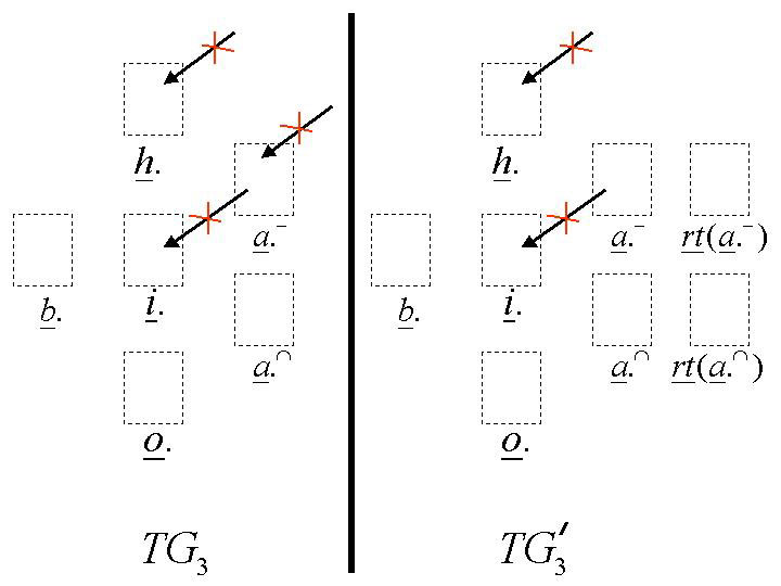
  Figure 9: Graph templates $TG_{3}$ and $TG_{3}^{\prime}$ used in the proof of Rule 3 of do-calculus rules theorem.

• Rule 3: Let ${\,\underline{a}\,}.^{-}$ and ${\,\underline{a}\,}.^{\cap}$ be abbreviations for the following sets of nodes:

  $${\,\underline{a}\,}.^{-}={\,\underline{a}\,}.-an({\,\underline{i}\,}.,G_{{\stackrel{{\scriptstyle\wedge}}{{{\,\underline{h}\,}}}}.})\;,$$ (42)

  and

  $${\,\underline{a}\,}.^{\cap}={\,\underline{a}\,}.\cap an({\,\underline{i}\,}.,G_{{\stackrel{{\scriptstyle\wedge}}{{{\,\underline{h}\,}}}}.})\;.$$ (43)

  Let ${\cal S}$ and ${\cal S}^{\prime}$ denote the following statements

  $${\cal S}=({\,\underline{b}\,}.\bot{\,\underline{a}\,}.|{\,\underline{h}\,}.,{\,\underline{i}\,}.)_{G_{3}}\mbox{ where }G_{3}=G_{{\stackrel{{\scriptstyle\wedge}}{{{\,\underline{h}\,}}}}.,\left[{\,\underline{a}\,}.^{-}\right]^{\wedge}}\;,$$ (44)

  and

  $${\cal S}^{\prime}=({\,\underline{b}\,}.\bot{\,\underline{a}\,}.,{\,\underline{rt}\,}({\,\underline{a}\,}.)|{\,\underline{h}\,}.,{\,\underline{i}\,}.)_{G^{\prime}_{3}}\mbox{ where }G_{3}^{\prime}=[G\leftarrow{\,\underline{rt}\,}({\,\underline{a}\,}.)]_{{\stackrel{{\scriptstyle\wedge}}{{{\,\underline{h}\,}}}}.}\;.$$ (45)

  By the D-sep Theorem, ${\cal S}^{\prime}$ implies, for all $b.,a.,rt({\,\underline{a}\,}.),h.,i.$,

  $$P(b.|a.,rt({\,\underline{a}\,}.),{\stackrel{{\scriptstyle\wedge}}{{h}}}.,i.)=P(b.|{\stackrel{{\scriptstyle\wedge}}{{h}}}.,i.)\;.$$ (46)

  But

  $$P(b.|a.,rt({\,\underline{a}\,}.)=1,{\stackrel{{\scriptstyle\wedge}}{{h}}}.,i.)=P(b.|{\stackrel{{\scriptstyle\wedge}}{{a}}}.,{\stackrel{{\scriptstyle\wedge}}{{h}}}.,i.)\;.$$ (47)

  So ${\cal S}^{\prime}$ implies Eq.(35). Hence we’ll be done with the proof if we can prove that ${\cal S}$ implies ${\cal S}^{\prime}$. Let’s prove this by proving the contrapositive $not({\cal S}^{\prime})$ implies $not({\cal S})$. If $not({\cal S}^{\prime})$, then there exists a path $\gamma$ which is unblocked at fixed ${\,\underline{h}\,}.{\,\underline{i}\,}.$, and which satisfies

  $$\gamma\in Path_{TG_{3}^{\prime}}({\,\underline{B}\,}<{\,\underline{A_{1}}\,}<{\,\underline{A_{2}}\,}<\ldots<{\,\underline{A_{n}}\,},{\,\underline{rt}\,}({\,\underline{A_{n}}\,}))\;,$$ (48)

  where ${\,\underline{B}\,}\in{\,\underline{b}\,}.$, ${\,\underline{A}\,}.\subset{\,\underline{a}\,}.$. Here ${\,\underline{A_{1}}\,}$ is the unique node in $\gamma$ that belongs to ${\,\underline{a}\,}.$ and is closest to ${\,\underline{B}\,}$. But then there is a shorter path $\gamma_{o}$ in $TG_{3}^{\prime}$ that is also unblocked at fixed ${\,\underline{h}\,}.,{\,\underline{i}\,}.$,

  $$\gamma_{o}\in Path_{T}({\,\underline{B}\,}<{\,\underline{A_{1}}\,},{\,\underline{rt}\,}({\,\underline{A_{1}}\,}))\;,$$ (49)

  where $T=TG_{3}^{\prime}$. If we can show that $\gamma_{o}$ is unblocked at fixed ${\,\underline{h}\,}.,{\,\underline{i}\,}.$ and also satisfies Eq.(49) with $T=TG_{3}$ instead of the bigger set $T=TG^{\prime}_{3}$, then we’ll be done. As shown in Fig.9, template $TG_{3}$ has the same bans as template $TG^{\prime}_{3}$ plus an additional ban on arrows entering ${\,\underline{a}\,}.^{-}$. So we need to show that $\gamma_{o}$ has no arrows entering ${\,\underline{a}\,}.^{-}$. Such an arrow would have to enter node ${\,\underline{A}\,}_{1}$. If ${\,\underline{A}\,}_{1}\in{\,\underline{a}\,}.^{\cap}$, then there is no arrow of $\gamma_{o}$ entering ${\,\underline{a}\,}.^{-}$ and we are done. If ${\,\underline{A}\,}_{1}\in{\,\underline{a}\,}.^{-}$, then there are two possibilities, either ${\,\underline{A}\,}_{1}\in col(\gamma_{o})$ or not.

  If ${\,\underline{A}\,}_{1}\notin col(\gamma_{o})$, since there is an arrow pointing from ${\,\underline{rt}\,}({\,\underline{A}\,}_{1})$ to ${\,\underline{A}\,}_{1}$, there must be an arrow pointing from ${\,\underline{A}\,}_{1}$ to a node outside of ${\,\underline{a}\,}.^{-}$. Thus, there are no arrows in $\gamma_{o}$ entering ${\,\underline{a}\,}.^{-}$ and we are done.

  If ${\,\underline{A}\,}_{1}\in col(\gamma_{o})$, then, since $\gamma_{o}$ is unblocked at fixed ${\,\underline{h}\,}.,{\,\underline{i}\,}.$, we must have $\overline{de}({\,\underline{A}\,}_{1})\cap({\,\underline{h}\,}.\cup{\,\underline{i}\,}.)\neq\emptyset$. But this is impossible since as shown by Fig.9, in $TG_{3}$ no arrow can enter ${\,\underline{h}\,}.$ and no arrow from ${\,\underline{a}\,}.^{-}$ can enter ${\,\underline{i}\,}.$.

.
QED

References

- [1] Daphne Koller, Nir Friedman, Probabilistic Graphical Models, Principles and Techniques (MIT Press, 2009)
- [2] J. Pearl, “Causal diagrams for empirical research”, R-218-B. (available in pdf format at J. Pearl’s website) Biometrika 82, 669-710 (1975)
- [3] J. Pearl, “The Do-Calculus Revisited”, Keynote Lecture Aug. 17, 2012, UAI-2012. (available in pdf format at J. Pearl’s website)