Distributed Minimum Cut Approximation

Abstract

We study the problem of computing approximate minimum edge cuts by distributed algorithms. We use a standard synchronous message passing model where in each round, $O(\log n)$ bits can be transmitted over each edge (a.k.a. the $\mathsf{CONGEST}$ model). We present a distributed algorithm that, for any weighted graph and any $\epsilon\in(0,1)$, with high probability finds a cut of size at most $O(\epsilon^{-1}\lambda)$ in $O(D)+\tilde{O}(n^{1/2+\epsilon})$ rounds, where $\lambda$ is the size of the minimum cut. This algorithm is based on a simple approach for analyzing random edge sampling, which we call the random layering technique. In addition, we also present another distributed algorithm, which is based on a centralized algorithm due to Matula [SODA ’93], that with high probability computes a cut of size at most $(2+\epsilon)\lambda$ in $\tilde{O}((D+\sqrt{n})/\epsilon^{5})$ rounds for any $\epsilon>0$.

The time complexities of our algorithms almost match the $\tilde{\Omega}(D+\sqrt{n})$ lower bound of Das Sarma et al. [STOC ’11], thus leading to an answer to an open question raised by Elkin [SIGACT-News ’04] and Das Sarma et al. [STOC ’11].

To complement our upper bound results, we also strengthen the $\tilde{\Omega}(D+\sqrt{n})$ lower bound of Das Sarma et al. by extending it to unweighted graphs. We show that the same lower bound also holds for unweighted multigraphs (or equivalently for weighted graphs in which $O(w\log n)$ bits can be transmitted in each round over an edge of weight $w$). These results even hold if the diameter is $D=O(\log n)$. For unweighted simple graphs, we show that even for networks of diameter $\tilde{O}\big{(}\frac{1}{\lambda}\cdot\sqrt{\frac{n}{\alpha\lambda}}\big{)}$ finding an $\alpha$-approximate minimum cut in networks of edge connectivity $\lambda$ or computing an $\alpha$-approximation of the edge connectivity requires time at least $\tilde{\Omega}\big{(}D+\sqrt{\frac{n}{\alpha\lambda}}\big{)}$.

1 Introduction

Finding minimum cuts or approximately minimum cuts are classical and fundamental algorithmic graph problems with many important applications. In particular, minimum edge cuts and their size (i.e., the edge connectivity) are relevant in the context of networks, where edge weights might represent link capacities and therefore edge connectivity can be interpreted as the throughput capacity of the network. Decomposing a network using small cuts helps designing efficient communication strategies and finding communication bottlenecks (see, e.g., [26, 19]). Both the exact and approximate variants of the minimum cut problem have received extensive attention in the domain of centralized algorithms (cf. Section 1.1 for a brief review of the results in the centralized setting). This line of research has led to (almost) optimal centralized algorithms with running times $\tilde{O}(m+n)$ [18] for the exact version and $O(m+n)$[23] for constant-factor approximations, where $n$ and $m$ are the numbers of nodes and edges, respectively.

As indicated by Elkin[6] and Das Sarma et al. [4], the problem has remained essentially open in the distributed setting. In the $\mathsf{LOCAL}$ model [25] where in each round, a message of unbounded size can be sent over each edge, the problem has a trivial time complexity of $\Theta(D)$ rounds, where $D$ is the (unweighted) diameter of the network. The problem is therefore more interesting and also practically more relevant in models where messages are of some bounded size $B$. The standard model incorporating this restriction is the $\mathsf{CONGEST}$ model [25], a synchronous message passing model where in each time unit, $B$ bits can be sent over every link (in each direction). It is often assumed that $B=\Theta(\log n)$. The only known non-trivial result is an elegant lower bound by Das Sarma et al. [4] showing that any $\alpha$-approximation of the minimum cut in weighted graphs requires at least $\Omega(D+\sqrt{n/(B\log n)})$ rounds.

Our Contribution:

We present two distributed minimum-cut approximation algorithms for undirected weighted graphs, with complexities almost matching the lower bound of [4]. We also extend the lower bound of [4] to unweighted graphs and multigraphs.

Our first algorithm, presented in Section 4, with high probability finds a cut of size at most $O(\varepsilon^{-1}{\lambda})$, for any $\epsilon\in(0,1)$ and where ${\lambda}$ is the edge connectivity, i.e., the size of the minimum cut in the network. The time complexity of this algorithm is $O(D)+O(n^{1/2+\epsilon}\log^{3}n\log\log n\log^{*}n)$. The algorithm is based on a simple and novel approach for analyzing random edge sampling, a tool that has proven extremely successful also for studying the minimum cut problem in the centralized setting (see, e.g., [19]). Our analysis is based on random layering, and we believe that the approach might also be useful for studying other connectivity-related questions. Assume that each edge $e\in E$ of an unweighted multigraph $G=(V,E)$ is independently sampled and added to a subset $E^{\prime}\subset E$ with probability $p$. For $p\leq\frac{1}{{\lambda}}$, the graph $G^{\prime}=(V,E^{\prime})$ induced by the sampled edges is disconnected with at least a constant probability (just consider one min-cut). In Section 3, we use random layering to show that if $p=\Omega(\frac{\log n}{{\lambda}})$, the sampled graph $G^{\prime}$ is connected w.h.p. This bound is optimal and was known previously, with two elegant proofs: [22] and [15]. Our proof is simple and self-contained and it serves as a basis for our algorithm in Section 4.

The second algorithm, presented in Section 5, finds a cut with size at most $(2+\varepsilon){\lambda}$, for any constant $\varepsilon>0$, in time $O((D+\sqrt{n}\log^{*}n)\log^{2}n\log\log n\cdot\frac{1}{\varepsilon^{5}})$. This algorithm combines the general approach of Matula’s centralized $(2+\varepsilon)$-approximation algorithm [23] with Thurimella’s algorithm for sparse edge-connectivity certificates[28] and with the famous random edge sparsification technique of Karger (see e.g., [15]).

To complement our upper bounds, we also extend the lower bound of Das Sarma et al. [4] to unweighted graphs and multigraphs. When the minimum cut problem (or more generally problems related to small edge cuts and edge connectivity) are in a distributed context, often the weights of the edges correspond to their capacities. It therefore seems reasonable to assume that over a link of twice the capacity, we can also transmit twice the amount of data in a single time unit. Consequently, it makes sense to assume that over an edge of weight (or capacity) $w\geq 1$, $O(w\log n)$ bits can be transmitted per round (or equivalently that such a link corresponds to $w$ parallel links of unit capacity). The lower bound of [4] critically depends on having links with (very) large weight over which in each round only $O(\log n)$ bits can be transmitted. We generalize the approach of [4] and obtain the same lower bound result as in [4] for the weaker setting where edge weights correspond to edge capacities (i.e., the setting that can be modeled using unweighted multigraphs). Formally, we show that if $Bw$ bits can be transmitted over every edge of weight $w\geq 1$, for every $\alpha\geq 1$ and sufficiently large $\lambda$, there are $\lambda$-edge-connected networks with diameter $O(\log n)$ on which computing an $\alpha$-approximate minimum cut requires time at least $\Omega\big{(}\sqrt{n/(B\log n)}\big{)}$. Further, for unweighted simple graphs with edge connectivity $\lambda$, we show that even for diameter $D=\big{(}\frac{1}{\lambda}\cdot\sqrt{n/(\alpha\lambda B\log n)}\big{)}$ finding an $\alpha$-approximate minimum cut or approximating the edge connectivity by a factor of $\alpha$ requires at least time $\Omega\big{(}\sqrt{n/(\alpha\lambda B\log n)}\big{)}$.

In addition, our technique yields a structural result about ${\lambda}$-edge-connected graphs with small diameter. We show that for every ${\lambda}>1$, there are ${\lambda}$-edge-connected graphs $G$ with diameter $O(\log n)$ such that for any partition of the edges of $G$ into spanning subgraphs, all but $O(\log n)$ of the spanning subgraphs have diameter $\Omega(n)$ (in the case of unweighted multigraphs) or $\Omega(n/{\lambda})$ (in the case of unweighted simple graphs). As a corollary, we also get that when sampling each edge of such a graph with probability $p\leq\gamma/\log n$ for a sufficiently small constant $\gamma>0$, with at least a positive constant probability, the subgraph induced by the sampled edges has diameter $\Omega(n)$ (in the case of unweighted multigraphs) and $\Omega(n/{\lambda})$ (in the case of unweighted simple graphs). The details about these results are deferred to Appendix D.

1.1 Related Work in the Centralized Setting

Starting in the 1950s [8, 5], the traditional approach to the minimum cut problem was to use max-flow algorithms (cf. [7] and [19, Section 1.3]). In the 1990s, three new approaches were introduced which go away from the flow-based method and provide faster algorithms: The first method, presented by Gabow[9], is based on a matroid characterization of the min-cut and it finds a min-cut in $O(m+{\lambda}^{2}n\log{\frac{n}{m}})$ steps, for any unweighted (but possibly directed) graph with edge connectivity ${\lambda}$. The second approach applies to (possibly) weighted but undirected graphs and is based on repeatedly identifying and contracting edges outside a min-cut until a min-cut becomes apparent (e.g., [24, 14, 19]). The beautiful random contraction algorithm (RCA) of Karger [14] falls into this category. In the basic version of RCA, the following procedure is repeated $O(n^{2}\log n)$ times: contract uniform random edges one by one until only two nodes remain. The edges between these two nodes correspond to a cut in the original graph, which is a min-cut with probability at least $1/O({n^{2}})$. Karger and Stein [19] also present a more efficient implementation of the same basic idea, leading to total running time of $O(n^{2}\log^{3}n)$. The third method, which again applies to (possibly) weighted but undirected graphs, is due to Karger[17] and is based on a “semiduality” between minimum cuts and maximum spanning tree packings. This third method leads to the best known centralized minimum-cut algorithm[18] with running time $O(m\log^{3}n)$.

For the approximation version of the problem (in undirected graphs), the main known results are as follows. Matula [23] presents an algorithm that finds a $(2+\varepsilon)$-minimum cut for any constant $\varepsilon>0$ in time $O((m+n)/\varepsilon)$. This algorithm is based on a graph search procedure called maximum adjacency search. Based on a modified version of the random contraction algorithm, Karger[16] presents an algorithm that finds a $(1+\varepsilon)$-minimum cut in time $O(m+n\log^{3}n/\varepsilon^{4})$.

2 Preliminaries

Notations and Definitions:

We usually work with an undirected weighted graph $G=(V,E,w)$, where $V$ is a set of $n$ vertices, $E$ is a set of (undirected) edges $e=\{v,u\}$ for $u,v\in V$, and $w:E\rightarrow\mathbb{R}^{+}$ is a mapping from edges $E$ to positive real numbers. For each edge $e\in E$, $w(e)$ denotes the weight of edge $e$. In the special case of unweighted graphs, we simply assume $w(e)=1$ for each edge $e\in E$.

For a given non-empty proper subset $C\subset V$, we define the cut $(C,V\setminus C)$ as the set of edges in $E$ with exactly one endpoint in set $C$. The size of this cut, denoted by $w(C)$ is the sum of the weights of the edges in set $(C,V\setminus C)$. The edge-connectivity ${\lambda}(G)$ of the graph is defined as the minimum size of $w(C)$ as $C$ ranges over all nonempty proper subsets of $V$. A cut $(C,V\setminus C)$ is called $\alpha$-minimum, for an $\alpha\geq 1$, if $w(C)\leq\alpha{\lambda}(G)$. When clear from the context, we sometimes use ${\lambda}$ to refer to $\lambda(G)$.

Communicaton Model and Problem Statements:

We use a standard message passing model (a.k.a. the $\mathsf{CONGEST}$ model[25]), where the execution proceeds in synchronous rounds and in each round, each node can send a message of size $B$ bits to each of its neighbors. A typically standard case is $B=\Theta(\log n)$.

For upper bounds, for simplicity we assume that $B=\Theta(\log n)$. For upper bounds, we further assume that $B$ is large enough so that a constant number of node identifiers and edge weights can be packed into a single message. For $B=\Theta(\log n)$, this implies that each edge weight $w(e)$ is at most (and at least) polynomial in $n$. W.l.o.g., we further assume that edge weights are normalized and each edge weight is an integer in range $\{1,\dots,n^{\Theta(1)}\}$. Thus, we can also view a weighted graph as a multi-graph in which all edges have unit weight and multiplicity at most $n^{\Theta(1)}$ (but still only $O(\log n)$ bits can be transmitted over all these parallel edges together).

For lower bounds, we assume a weaker model where $B\cdot w(e)$ bits can be sent in each round over each edge $e$. To ensure that at least $B$ bits can be transmitted over each edge, we assume that the weights are scaled such that $w(e)\geq 1$ for all edges. For integer weights, this is equivalent to assuming that the network graph is an unweighted multigraph where each edge $e$ corresponds to $w(e)$ parallel unit-weight edges.

In the problem of computing an $\alpha$-approximation of the minimum cut, the goal is to find a cut $(C^{*},V\setminus C^{*})$ that is $\alpha$-minimum. To indicate this cut in the distributed setting, each node $v$ should know whether $v\in C^{*}$. In the problem of $\alpha$-approximation of the edge-connectivity, all nodes must output an estimate $\tilde{{\lambda}}$ of ${\lambda}$ such that $\tilde{{\lambda}}\in[{\lambda},{\lambda}\alpha]$. In randomized algorithms for these problems, time complexities are fixed deterministically and the correctness guarantees are required to hold with high probability.

2.1 Black-Box Algorithms

In this paper, we make frequent use of a connected component identification algorithm due to Thurimella [28], which itself builds on the minimum spanning tree algorithm of Kutten and Peleg[21]. Given a graph $G(V,E)$ and a subgraph $H=(V,E^{\prime})$ such that $E^{\prime}\subseteq E$, Thurimella’s algorithm identifies the connected components of $H$ by assigning a label $\ell(v)$ to each node $v\in V$ such that two nodes get the same label iff they are in the same connected component of $H$. The time complexity of the algorithm is $O(D+\sqrt{n}\log^{*}{n})$ rounds, where $D$ is the (unweighted) diameter of $G$. Moreover, it is easy to see that the algorithm can be made to produce labels $\ell(v)$ such that $\ell(v)$ is equal to the smallest (or the largest) id in the connected component of $H$ that contains $v$. Furthermore, the connected component identification algorithm can also be used to test whether the graph $H$ is connected (assuming that $G$ is connected). $H$ is not connected if and only if there is an edge $\left\{u,v\right\}\in E$ such that $\ell(u)\neq\ell(v)$. If some node $u$ detects that for some neighbor $v$ (in $G$), $\ell(u)\neq\ell(v)$, $u$ broadcasts not connected. Connectivity of $H$ can therefore be tested in $D$ additional rounds. We refer to this as Thurimella’s connectivity-tester algorithm. Finally, we remark that the same algorithms can also be used to solve $k$ independent instances of the connected component identification problem or $k$ independent instances of the connectivity-testing problem in $O(D+k\sqrt{n}\log^{*}{n})$ rounds. This is achieved by pipelining the messages of the broadcast parts of different instances.

3 Edge Sampling and The Random Layering Technique

Here, we study the process of random edge-sampling and present a simple technique, which we call random layering, for analyzing the connectivity of the graph obtained through sampling. This technique also forms the basis of our min-cut approximation algorithm presented in the next section.

Edge Sampling

Consider an arbitrary unweighted multigraph $G=(V,E)$. Given a probability $p\in[0,1]$, we define an edge sampling experiment as follows: choose subset $S\subseteq E$ by including each edge $e\in E$ in set $S$ independently with probability $p$. We call the graph $G^{\prime}=(V,S)$ the sampled subgraph.

We use the random layering technique to answer the following network reliability question: “How large should $p$ be, as a function of minimum-cut size ${\lambda}$, so that the sampled graph is connected w.h.p.?” Considering just one cut of size ${\lambda}$ we see that if $p\leq\frac{1}{{\lambda}}$, then the probability that the sampled subgraph is connected is at most $\frac{1}{e}$. We show that $p\geq\frac{20\log n}{{\lambda}}$ suffices so that the sampled subgraph is connected w.h.p. Note that this is non-trivial as a graph has exponential many cuts. It is easy to see that this bound is asymptotically optimal [22].

Theorem 3.1.

Consider an arbitrary unweighted multigraph $G=(V,E)$ with edge connectivity ${\lambda}$ and choose subset $S\subseteq E$ by including each edge $e\in E$ in set $S$ independently with probability $p$. If $p\geq\frac{20\log n}{{\lambda}}$, then the sampled subgraph $G^{\prime}=(V,S)$ is connected with probability at least $1-\frac{1}{n}$.

We remark that this result was known prior to this paper, via two different proofs by Lomonosov and Polesskii [22] and Karger[15]. The Lomonosov-Polesskii proof [22] uses an interesting coupling argument and shows that among the graphs of a given edge-connectivity ${\lambda}$, a cycle of length $n$ with edges of multiplicity ${\lambda}/2$ has the smallest probability of remaining connected under random sampling. Karger’s proof[15] uses the powerful fact that the number of $\alpha$-minimum cuts is at most $O(n^{2\alpha})$ and then uses basic probability concentration arguments (Chernoff and union bounds) to show that, w.h.p., each cut has at least one sampled edge. There are many known proofs for the $O(n^{2\alpha})$ upper bound on the number of $\alpha$-minimum cuts (see [18]); an elegant argument follows from Karger’s random contraction algorithm[14].

Our proof of Theorem 3.1 is simple and self-contained, and it is the only one of the three approaches that extends to the case of random vertex failures [2, Theorem 1.5].

Proof of Theorem 3.1.

Let $L=20\log n$. For each edge $e\in E$, we independently choose a uniform random layer number from the set $\{1,2,\dots,L\}$. Intuitively, we add the sampled edges layer by layer and show that with the addition of the sampled edges of each layer, the number of connected components goes down by at least a constant factor, with at least a constant probability, and independently of the previous layers. After $L=\Theta(\log n)$ layers, connectivity is achieved w.h.p.

We start by presenting some notations. For each $i\in\{1,\dots,L\}$, let $S_{i}$ be the set of sampled edges with layer number $i$ and let $S_{i-}=\bigcup_{j=1}^{i}S_{j}$, i.e., the set of all sampled edges in layers $\{1,\dots,i\}$. Let $G_{i}=(V,S_{i-})$ and let $M_{i}$ be the number of connected components of graph $G_{i}$. We show that $M_{L}=1$, w.h.p.

For any $i\in[1,L-1]$, since $S_{i-}\subseteq S_{(i+1)-}$, we have $M_{i+1}\leq M_{i}$. Consider the indicator variable ${X}_{i}$ such that ${X}_{i}=1$ iff $M_{i+1}\leq 0.87M_{i}$ or $M_{i}=1$. We show the following claim, after which, applying a Chernoff bound completes the proof.

Claim 3.2.

For all $i\in[1,L-1]$ and $T\subseteq E$, we have $\Pr[X_{i}=1|S_{i-}=T]\geq 1/2$.

To prove this claim, we use the principle of deferred decisions[20] to view the two random processes of sampling edges and layering them. More specifically, we consider the following process: first, each edge is sampled and given layer number $1$ with probability $p/L$. Then, each remaining edge is sampled and given layer number $2$ with probability $\frac{p/L}{1-p/L}\geq p/L$. Similarly, after determining the sampled edges of layers $1$ to $i$, each remaining edge is sampled and given layer number $i+1$ with probability $\frac{p/L}{1-(i\,p)/L}\geq p/L$. After doing this for $L$ layers, any remaining edge is considered not sampled and it receives a random layer number from $\{1,2,\dots,L\}$. It is easy to see that in this process, each edge is independently sampled with probability exactly $p$ and each edge $e$ gets a uniform random layer number from $\{1,2,\dots,L\}$, chosen independently of the other edges and also independently of whether $e$ is sampled or not.

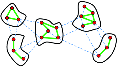
Figure 1: Graph $G_{i}$ and its connected components. The green solid links represent edges in $S_{i-}$ and the blue dashed links represent $E\setminus S_{i-}$.

Fix a layer $i\in[1,\dots,L-1]$ and a subset $T\subseteq E$. Let $S_{i-}=T$ and consider graph $G_{i}=(V,S_{i-})$. Figure 1 presents an example graph $G_{i}$ and its connected components. If $M_{i}=1$ meaning that $G_{i}$ is connected, then $X_{i}=1$. Otherwise, suppose that $M_{i}\geq 2$. For each component $\mathcal{C}$ of $G_{i}$, call the component bad if $(\mathcal{C},V\setminus\mathcal{C})\cap S_{i+1}=\emptyset$. That is, $\mathcal{C}$ is bad if after adding the sampled edges of layer $i+1$, $\mathcal{C}$ does not get connected to any other component. We show that $\Pr[\mathcal{C}\textit{ is bad}]\leq\frac{1}{e}$.

Since $G$ is ${\lambda}$-edge connected, we have $w(C)\geq{\lambda}$. Moreover, none of the edges in $(\mathcal{C},V\setminus\mathcal{C})$ is in $S_{i-}$. Thus, using the principle of deferred decisions as described, each of the edges of the cut $(\mathcal{C},V\setminus\mathcal{C})$ has probability $\frac{p/L}{1-(i\,p)/L}\geq p/L$ to be sampled and given layer number $i+1$, i.e., to be in $S_{i+1}$. Since $p\geq\frac{20\log n}{{\lambda}}$, the probability that none of the edges $(\mathcal{C},V\setminus\mathcal{C})$ is in set $S_{i+1}$ is at most $(1-p/L)^{{\lambda}}\leq 1/e$. Thus, $\Pr[\mathcal{C}\textit{ is bad}]\leq 1/e$.

Now let $Z_{i}$ be the number of bad components of $G_{i}$. Since each component is bad with probability at most $1/e$, we have $\mathbb{E}[Z_{i}]\leq M_{i}/e$. Using Markov’s inequality, we get $\Pr[Z_{i}\geq 2M_{i}/e]\leq 1/2$. Since each component that is not bad gets connected to at least one other component (when we look at graph $G_{i+1}$), we have $M_{i+1}\leq Z_{i}+\frac{(M_{i}-Z_{i})}{2}=\frac{M_{i}+Z_{i}}{2}$. Therefore, with probability at least $1/2$, we have $M_{i+1}\leq\frac{1+2/e}{2}M_{i}<0.87M_{i}$. This means that $\Pr[X_{i}=1]\geq 1/2$, which concludes the proof of the claim.

Now using the claim, we get that $\mathbb{E}[\sum_{i=1}^{L-1}X_{i}]\geq 10\log n$. A Chernoff bound then shows that $\Pr[\sum_{i=1}^{L-1}X_{i}\geq 5\log n]\geq 1-\frac{1}{n}$. This means that w.h.p, $M_{L}\leq\frac{n}{2^{\log n}}=1$. That is, w.h.p, $G_{L}=(V,S)=(V,S_{L-})=G^{\prime}$ is connected. ∎

Theorem 3.1 provides a very simple approach for finding an $O(\log n)$-approximation of the edge connectivity of a network graph $G$ in $O(D+\sqrt{n}\log^{2}n\log^{*}n)$ rounds, simply by trying exponentially growing sampling probabilities and checking the connectivity. The proof appears in Appendix A. We note that a similar basic approach has been used to approximate the size of min-cut in the streaming model [1].

Corollary 3.3.

There exists a distributed algorithm that for any unweighted multi-graph $G=(V,E)$, in $O(D+\sqrt{n}\log^{2}n\log^{*}n)$ rounds, finds an approximation $\tilde{{\lambda}}$ of the edge connectivity such that $\tilde{{\lambda}}\in[{\lambda},{\lambda}\cdot\Theta(\log n)]$ with high probability.

4 Min-Cut Approximation by Random Layering

Now we use random layering to design a min-cut approximation algorithm. We present the outline of the algorithm and its key parts in Subsections 4.1 and 4.2. Then, in Subsection 4.3, we explain how to put these parts together to prove the following theorem:

Theorem 4.1.

There is a distributed algorithm that, for any $\epsilon\in(0,1)$, finds an $O(\epsilon^{-1})$-minimum cut in $O(D)+O(n^{0.5+\epsilon}\log^{3}n\log\log n\log^{*}n)$ rounds, w.h.p.

4.1 Algorithm Outline

The algorithm is based on closely studying the sampled graph when the edge-sampling probability is between the two extremes of $\frac{1}{{\lambda}}$ and $\frac{\Theta(\log n)}{{\lambda}}$. Throughout this process, we identify a set $\mathcal{F}$ of $O(n\log n)$ cuts such that, with at least a ‘reasonably large probability’, $\mathcal{F}$ contains at least one ‘small’ cut.

The Crux of the Algorithm:

Sample edges with probability $p=\frac{\epsilon\log n}{2{\lambda}}$ for a small $\epsilon\in(0,1)$. Also, assign each edge to a random layer in $[1,\dots,L]$, where $L=20\log n$. For each layer $i\in[1,\dots,L-1]$, let $S_{i}$ be the set of sampled edges of layer $i$ and let $S_{i-}=\bigcup_{j=1}^{i}S_{j}$. For each layer $i\in[1,\dots,L-1]$, for each component $\mathcal{C}$ of graph $G_{i}=(V,S_{i-})$, add the cut $(\mathcal{C},V\setminus\mathcal{C})$ to the collection $\mathcal{F}$. Since in each layer we add at most $n$ new cuts and there are $L=O(\log n)$ layers, we collect $O(n\log n)$ cuts in total.

We show that with probability at least $n^{-\epsilon}/2$, at least one of the cuts in $\mathcal{F}$ is an $O(\epsilon^{-1})$-minimum cut. Note that thus repeating the experiment for $\Theta(n^{\epsilon}\log n)$ times is enough to get that an $O(\epsilon^{-1})$-minimum cut is found w.h.p.

Theorem 4.2.

Consider performing the above sampling and layering experiment with edge sampling probability $p=\frac{\epsilon\log n}{2{\lambda}}$ for $\epsilon\in(0,1)$ and $L=20\log n$ layers. Then, $\Pr[\mathcal{F}\textit{ contains an }O(\epsilon^{-1})\textit{-minimum cut}]\geq n^{-\epsilon}/2.$

Proof.

Fix an edge sampling probability $p=\frac{\epsilon\log n}{2{\lambda}}$ for an $\epsilon\in(0,1)$ and let $\alpha=40\epsilon^{-1}$. We say that a sampling and layering experiment is successful if $\mathcal{F}$ contains an $\alpha$-minimum cut or if the sampled graph $G_{L}=(V,S_{L-})$ is connected. We first show that each experiment is successful with probability at least $1-\frac{1}{n}$. The proof of this part is very similar to that of Theorem 3.1.

For an arbitrary layer number $1\leq i\leq L-1$, consider graph $G_{i}=(V,S_{i-})$. If $M_{i}=1$ meaning that $G_{i}$ is connected, then $G_{L}$ is also connected. Thus, in that case, the experiment is successful and we are done. In the more interesting case, suppose $M_{i}\geq 2$. For each component $\mathcal{C}$ of $G_{i}$, consider the cut $(\mathcal{C},V\setminus\mathcal{C})$. If any of these cuts is $\alpha$-minimum, then the experiment is successful as then, set $\mathcal{F}$ contains an $\alpha$-minimum cut. On the other hand, suppose that for each component $\mathcal{C}$ of $G_{i}$, we have $w(C)\geq\alpha{\lambda}$. Then, for each such component $\mathcal{C}$, each of the edges of cut $(\mathcal{C},V\setminus\mathcal{C})$ has probability $\frac{p/L}{1-(i\,p)/L}\geq p/L$ to be in set $S_{i+1}$ and since $w(\mathcal{C})\geq\alpha{\lambda}$, where $\alpha=20\epsilon^{-1}$, the probability that none of the edges of this cut in set $S_{i+1}$ is at most $(1-p/L)^{\alpha{\lambda}}\leq e^{\frac{p}{L}\cdot\alpha{\lambda}}=e^{-\frac{\epsilon\log n}{2{\lambda}}\cdot\frac{1}{L}\cdot\frac{40}{\epsilon}\cdot{\lambda}}=1/e$. Hence, the probability that component $\mathcal{C}$ is bad as defined in the proof of Theorem 3.1 (i.e., in graph $G_{i+1}$, it does not get connected to any other component) is at most $1/e$. The rest of the proof can be completed exactly as the last paragraph of of the proof of Theorem 3.1, to show that

$$\Pr[\textit{successful experiment}]\geq 1-{1}/{n}.$$

Thus we have a bound on the probability that $\mathcal{F}$ contains an $\alpha$-minimum cut or that the sampled graph $G=(V,S_{L-})$ is connected. However, in Theorem 4.2, we are only interested in the probability of $\mathcal{F}$ containing an $\alpha$-minimum cut. Using a union bound, we know that

$$\Pr[\textit{successful experiment}]\leq\Pr[\mathcal{F}\textit{ contains an }\alpha\textit{-min cut}]+\Pr[G_{L}\textit{ is connected}].$$

On the other hand,

$$\Pr[G_{L}\textit{ is connected}]\leq 1-n^{-\epsilon}.$$

This is because, considering a single mininmum cut of size ${\lambda}$, the probability that none of the edges of this cut are sampled, in which case the sampled subgraph is disconnected, is $(1-\frac{\epsilon\log n}{2{\lambda}})^{{\lambda}}\geq n^{-\epsilon}$. Hence, we can conclude that

$$\quad\,\Pr[\mathcal{F}\textit{ contains an }\alpha\textit{-min cut}]\geq(1-{1}/{n})-(1-n^{-\epsilon})=n^{-\epsilon}-{1}/{n}\geq n^{-\epsilon}/2.$$

∎

Remark: It was brought to our attention that the approach of Theorem 4.2 bears some cosmetic resemblance to the technique of Goel, Kapralov and Khanna [11]. As noted by Kapralov[13], the approaches are fundamentally different; the only similarity is having $O(\log n)$ repetitions of sampling. In [11], the objective is to estimate the strong-connectivity of edges via a streaming algorithm. See [11] for related definitions and note also that strong-connectivity is (significantly) different from (standard) connectivity. In a nutshell, [11] uses $O(\log n)$ iterations of sub-sampling, each time further sparsifying the graph until at the end, all edges with strong-connectivity less than a threshold are removed (and identified) while edges with strong connectivity that is a $\Theta(\log n)$ factor larger than the threshold are preserved (proven via Benczur-Karger’s sparsification).

4.2 Testing Cuts

So far we know that $\mathcal{F}$ contains an $\alpha$-minimum cut with a reasonable probability. We now need to devise a distributed algorithm to read or test the sizes of the cuts in $\mathcal{F}$ and find that $\alpha$-minimum cut, in $O(D)+\tilde{O}(\sqrt{n})$ rounds. In the remainder of this section, we explain our approach to this part.

Consider a layer $i$ and the graph $G_{i}=(V,S_{i-})$. For each component $\mathcal{C}$ of $G_{i}$, $diam(\mathcal{C})$ rounds is enough to read the size of the cut $(\mathcal{C},V\setminus\mathcal{C})$ such that all the nodes in component $\mathcal{C}$ know this size. However, $diam(\mathcal{C})$ can be considerably larger than $D=diam(G)$ and thus, this method would not lead to a round complexity of $\tilde{O}(D+\sqrt{n})$. To overcome this problem, notice that we do not need to read the exact size of the cut $(\mathcal{C},V\setminus\mathcal{C})$. Instead, it is enough to devise a test that passes w.h.p. if $w(C)\leq\alpha{\lambda}$, and does not pass w.h.p. if $w(C)\geq(1+\delta)\alpha{\lambda}$, for a small constant $\delta\in(0,1/4)$. In the distributed realization of such a test, it would be enough if all the nodes in $\mathcal{C}$ consistently know whether the test passed or not. Next, we explain a simple algorithm for such a test. This test itself uses random edge sampling. Given such a test, in each layer $i\in[1,\dots,L-1]$, we can test all the cuts and if any cut passes the test, meaning that, w.h.p., it is a $((1+\delta)\alpha)$-minimum cut, then we can pick such a cut.

Lemma 4.3.

Given a subgraph $G^{\prime}=(V,E^{\prime})$ of the network graph $G=(V,E)$, a threshold $\kappa$ and $\delta\in(0,1/4)$, there exists a randomized distributed cut-tester algorithm with round complexity $\Theta\big{(}D+\frac{1}{\delta^{2}}\sqrt{n}\log n\log^{*}n\big{)}$ such that, w.h.p., for each node $v\in V$, we have: Let $\mathcal{C}$ be the connected component of $G^{\prime}$ that contains $v$. If $w(\mathcal{C})\leq\kappa/(1+\delta)$, the test passes at $v$, whereas if $w(\mathcal{C})\geq\kappa(1+\delta)$, the test does not pass at $v$.

For pseudo-code, we refer to Appendix B. We first run Thurimella’s connected component identification algorithm (refer to Section 2.1) on graph $G$ for subgraph $G^{\prime}$, so that each node $v\in V$ knows the smallest id in its connected component of graph $G^{\prime}$. Then, each node $v$ adopts this label $componentID$ as its own id (temporarily). Thus, nodes of each connected component of $G^{\prime}$ will have the same id. Now, the test runs in $\Theta(\log^{2}n/\delta^{2})$ experiments, each as follows: in the $j^{th}$ experiment, for each edge $e\in E\setminus E^{\prime}$, put edge $e$ in set $E_{j}$ with probability $p^{\prime}=1-2^{-\,\frac{1}{\kappa}}$. Then, run Thurimella’s algorithm on graph $G$ with subgraph $H_{j}=(V,E^{\prime}\cup E_{j})$ and with the new ids twice, such that at the end, each node $v$ knows the smallest and the largest id in its connected component of $H_{j}$. Call these new labels $\ell^{min}_{j}(v)$ and $\ell^{max}_{j}(v)$, respectively. For a node $v$ of a component $\mathcal{C}$ of $G_{i}$, we have that $\ell^{min}_{j}(v)\neq v.id$ or $\ell^{max}_{j}(v)\neq v.id$ iff at least one of the edges of cut $(\mathcal{C},V\setminus\mathcal{C})$ is sampled in $E_{j}$, i.e., $(\mathcal{C},V\setminus\mathcal{C})\cap E_{j}\neq\emptyset$. Thus, each node $v$ of each component $\mathcal{C}$ knows whether $(\mathcal{C},V\setminus\mathcal{C})\cap E_{j}\neq\emptyset$ or not. Moreover, this knowledge is consistent between all the nodes of component $\mathcal{C}$. After $\Theta(\log n/\delta^{2})$ experiments, each node $v$ of component $\mathcal{C}$ considers the test passed iff $v$ noticed $(\mathcal{C},V\setminus\mathcal{C})\cap E_{j}\neq\emptyset$ in at most half of the experiments. We defer the calculations of the proof of Lemma 4.3 to Appendix B.

4.3 Putting the Pieces Together

We now explain how to put together the pieces presented in the previous subsections to get the claim of Theorem 4.1.

Proof of Theorem 4.1.

For simplicity, we first explain an $O(\varepsilon^{-1})$ minimum-cut approximation algorithm with time complexity $O((D+\sqrt{n}\log^{*}n\log n)n^{\epsilon}\log^{2}n\log\log n)$. Then, explain how to reduce it to the claimed bound of $O(D)+O(n^{0.5+\epsilon}\log^{3}n\log\log n\log^{*}n)$ rounds.

We first find an $O(\log n)$ approximation $\tilde{{\lambda}}$ of ${\lambda}$, using Corollary 3.3, in time $O(D)+O(\sqrt{n}\log^{*})\log^{2}n)$. This complexity is subsumed by the complexity of the later parts. After this, we use $\Theta(\log\log n)$ guesses for a $2$-approximation of ${\lambda}$ in the form ${\lambda}^{\prime}_{i}=\tilde{C}2^{i}$ where $i\in[-\Theta(\log\log n),\Theta(\log\log n)]$. For each such guess ${\lambda}^{\prime}_{i}$, we have $n^{\epsilon}\log n$ epochs as follows:

In each epoch, we sample edges with probability $p=\frac{\epsilon\log n}{2{\lambda}^{\prime}}$ and assign each edge to a random layer in $[1,\dots,L]$, where $L=20\log n$. For each layer $i\in[1,\dots,L-1]$, we let $S_{i}$ be the set of sampled edges of layer $i$ and let $S_{i-}=\cup_{j=1}^{i}S_{j}$. Then, for each $i\in[1,\dots,L]$, we use the Cut-Tester Algorithm (see Section 4.2) on graph $G$ with subgraph $G_{i}=(V,S_{i-})$, threshold $\kappa=50{\lambda}^{\prime}/\epsilon$, and with parameter $\delta=1/8$. This takes $O((D+\sqrt{n}\log n\log^{*}n)\log n)$ rounds (for each layer). If in a layer, a component passes the test, it means its cut has size at most $O({\lambda}^{\prime}/\epsilon)$, with high probability. To report the results of the test, we construct a BFS tree rooted in a leader in $O(D)$ rounds and we convergecast the minimum $componentID$ that passed the test, in time $O(D)$. We then broadcast this $componentID$ to all nodes and all nodes that have this $componentID$ define the cut that is $O({\lambda}^{\prime}/\epsilon)$-minimum, with high probability.

Over all the guesses, we know that there is a guess ${\lambda}^{\prime}_{j}$ that is a $2$-approximation of ${\lambda}$. In that guess, from Theorem 4.2 and a Chernoff bound, we know that at least one cut that is an $O(\epsilon^{-1})$-minimum cut will pass the test. We stop the process in the smallest guess for which a cut passes the test.

Finally, to reduce the time complexity to $O(D)+O(n^{0.5+\epsilon}\log^{3}n\log\log n\log^{*}n)$ rounds, note that we can parallelize (i.e., pipeline) the $\Theta(n^{\epsilon}\log^{2}n\log\log n)$ runs of Cut-Testing algorithm, which come from $\Theta(\log\log n)$ guesses ${\lambda}^{\prime}_{i}$, $n^{\epsilon}\log n$ epochs for each guess, and $\Theta(\log n)$ layers in each epoch. We can do this pipe-lining simply because these instances of Cut-Testing do not depend on the outcomes of each other and $k$ instances of Thurimella’s algorithms can be run together in time $O(D+k\sqrt{n}\log^{*}n)$ rounds (refer to Section 2.1). To output the final cut, when doing the convergecast of the Cut-Testing results on the BFS, we append the edge-connectivity guess ${\lambda}^{\prime}_{j}$, epoch number, and layer number to the $componentID$. Then, instead of taking minimum on just $componentID$, we choose the $componentID$ that has the smallest tuple (guess ${\lambda}^{\prime}_{j}$, epoch number, layer number, $componentID$). Note that the smallest guess ${\lambda}^{\prime}_{j}$ translates to the smallest cut size, and the other parts are simply for tie-breaking. ∎

5 Min-Cut Approximation via Matula’s Approach

In [23], Matula presents an elegant centralized algorithm that for any constant $\varepsilon>0$, finds a $(2+\varepsilon)$-min-cut in $O(|V|+|E|)$ steps. Here, we explain how with the help of a few additional elements, this general approach can be used in the distributed setting, to find a $(2+\varepsilon)$-minimum cut in $O\big{(}(D+\sqrt{n}\log^{*}n)\log^{2}n\log\log n\cdot\frac{1}{\varepsilon^{5}}\big{)}$ rounds. We first recap the concept of sparse certificates for edge connectivity.

Definition 5.1.

For a given unweighted multi-graph $H=(V_{H},E_{H})$ and a value $k>0$, a set $E^{*}\subseteq E_{H}$ of edges is a sparse certificate for $k$-edge-connectivity of $H$ if (1) $|E^{*}|\leq k|V_{H}|$, and (2) for each edge $e\in E_{H}$, if there exists a cut $(\mathcal{C},V\setminus\mathcal{C})$ of $H$ such that $|(\mathcal{C})|\leq k$ and $e\in(\mathcal{C},V\setminus\mathcal{C})$, then we have $e\in E^{*}$.

Thurimella [28] presents a simple distributed algorithm that finds a sparse certificate for $k$-edge-connectivity of a network graph $G$ in $O(k(D+\sqrt{n}\log^{*}n))$ rounds. With simple modifications, we get a generalized version, presented in Lemma 5.2. Details of these modification appear in Appendix C.

Lemma 5.2.

Let $E_{c}$ be a subset of the edges of the network graph $G$ and define the virtual graph $G^{\prime}=(V^{\prime},E^{\prime})$ as the multi-graph that is obtained by contracting all the edges of $G$ that are in $E_{c}$. Using the modified version of Thurimella’s certificate algorithm, we can find a set $E^{*}\subseteq E\setminus E_{c}$ that is a sparse certificate for $k$-edge-connectivity of $G^{\prime}$, in $O(k(D+\sqrt{n}\log^{*}n))$ rounds.

Following the approach of Matula’s centralized algorithm [23], and with the help of the sparse certificate algorithm of Lemma 5.2 and the random sparsification technique of Karger [15], we get the following result.

Theorem 5.3.

There is a distributed algorithm that, for any constant $\varepsilon>0$, finds a $(2+\varepsilon)$-minimum cut in $O((D+\sqrt{n}\log^{*}n)\log^{2}n\log\log n\cdot\frac{1}{\varepsilon^{5}})$ rounds.

Algorithm 1 $(2+\varepsilon)$-minimum cut approximation: Matula’s Approach

1:Given a $(1+\varepsilon/10)$-factor approximation $\tilde{{\lambda}}$ of ${\lambda}$

2:

3:$E_{c}\leftarrow\emptyset$, $E^{*}\leftarrow E$, $\eta_{old}\leftarrow n$, $\eta_{new}\leftarrow 1$

4:while ($\eta\geq 2$) & ($\eta_{new}\leq\eta_{old}(1-\varepsilon/10)$) do

5:    $E_{c}\leftarrow E\setminus E^{*}$

6:    $E^{*}\leftarrow$ a sparse certificate for $\tilde{{\lambda}}(1+\varepsilon/5)$-edge-connectivity of graph $G^{\prime}=(V^{\prime},E^{\prime})$ obtained by contracting edges of $E_{c}$

7:    $\eta_{new}\leftarrow$ number of connected components of subgraph $H=(V,E\setminus E^{*})$

8:endwhile

9:Test cuts defined by connected components of graph $H=(V,E\setminus E^{*})$ versus threshold $\kappa=\tilde{{\lambda}}(2+\varepsilon/3)$

10:Output the component that passes the test and contains the smallest id between such components

Proof of Theorem 5.3.

We assume that nodes know a $(1+\varepsilon/10)$-factor approximation $\tilde{{\lambda}}$ of the edge connectivity ${\lambda}$, and explain a distributed algorithm with round complexity $O((D+\sqrt{n}\log^{*}n)\log^{2}n\cdot\frac{1}{\varepsilon^{4}})$. Note that this assumption can be removed at the cost of a $\Theta(\frac{\log\log n}{\log{(1+\varepsilon/10)}})=\Theta(\log\log n\cdot\frac{1}{\varepsilon})$ factor increase in round complexity by trying $\Theta(\frac{\log\log n}{\varepsilon})$ exponential guesses $\tilde{{\lambda}}(1+\varepsilon/10)^{i}$ for $i\in[0,\Theta(\frac{\log\log n}{\varepsilon})]$ where $\tilde{{\lambda}}$ is an $O(\log n)$-approximation of the edge-connectivity, which can be found by Corollary 3.3.

For simplicity, we first explain an algorithm that finds a $(2+\varepsilon)$-minimum cut in $O(\lambda(D+\sqrt{n}\log^{*}n)\log n\cdot\frac{1}{\varepsilon^{2}})$ rounds. Then, we explain how to reduce the round complexity to $O((D+\sqrt{n}\log^{*}n)\log^{2}n\cdot\frac{1}{\varepsilon^{4}})$. A pseudo-code is presented in Algorithm 10.

First, we compute a sparse certificate $E^{*}$ for $\tilde{{\lambda}}(1+\varepsilon/5)$-edge-connectivity for $G$, using Thurimella’s algorithm. Now consider the graph $H=(V,E\setminus E^{*})$. We have two cases: either (a) $H$ has at most $|V|(1-\varepsilon/10)$ connected components, or (b) there is a connected component $\mathcal{C}$ of $H$ such that $w(\mathcal{C})\leq\frac{2{\lambda}(1+\varepsilon/10)(1+\varepsilon/5)}{1-\varepsilon/10}\leq(2+\varepsilon){\lambda}$. Note that if (a) does not hold, case (b) follows because $H$ has at most $(1+\varepsilon/5)\tilde{{\lambda}}|V|$ edges.

In Case (b), we can find a $(2+\varepsilon)$-minimum cut by testing the connected components of $H$ versus threshold $\kappa=\tilde{{\lambda}}(2+\varepsilon/3)$, using the Cut-Tester algorithm presented in Lemma 4.3. In Case (a), we can solve the problem recursively on the virtual graph $G^{\prime}=(V^{\prime},E^{\prime})$ that is obtained by contracting all the edges of $G$ that are in $E_{c}=E\setminus E^{*}$. Note that this contraction process preserves all the cuts of size at most $\tilde{{\lambda}}(1+\varepsilon/5)\geq{\lambda}$ but reduces the number of nodes (in the virtual graph) at least by a $(1-\varepsilon/10)$-factor. Consequently, $O(\log(n)/\varepsilon)$ recursions reduce the number of components to at most $2$ while preserving the minimum cut.

The dependence on ${\lambda}$ can be removed by considering the graph $G_{S}=(V,E_{S})$, where $E_{S}$ independently contains every edge of $G$ with probability $\Theta\big{(}\frac{\log n}{\varepsilon^{2}{\lambda}}\big{)}$. It can be shown that the edge connectivity of $G_{S}$ is $\Theta(\log(n)/\varepsilon^{2})$ and a minimum edge cut of $G_{S}$ gives a $(1+O(\varepsilon))$-minimum edge cut of $G$.

We now explain how to remove the dependence on ${\lambda}$ from the time complexity. Let $E_{S}$ be a subset of the edges of $G=(V,E)$ where each $e\in E$ is independently included in $E_{S}$ with probability $p=\frac{100\log n}{\varepsilon^{2}}\cdot\frac{1}{{\lambda}}$. Then, using the edge-sampling result of Karger [15, Theorem 2.1], we know that with high probability, for each $\mathcal{C}\subseteq V$, we have

$$(1-\varepsilon/3)\cdot|(\mathcal{C},V\setminus\mathcal{C})|\cdot p\leq|(\mathcal{C},V\setminus\mathcal{C})\cap E_{S}|\leq(1+\varepsilon/3)\cdot|(\mathcal{C},V\setminus\mathcal{C})|\cdot p.$$

Hence, in particular, we know that graph $G_{new}=(V,E_{S})$ has edge connectivity at least ${\lambda}p(1-\varepsilon/3)$ and at most ${\lambda}p(1+\varepsilon/3)$, i.e., ${\lambda}_{new}=\Theta(\log n\cdot\frac{1}{\varepsilon^{2}})$. Moreover, for every cut $(\mathcal{C},V\setminus\mathcal{C})$ that is a $(1+\varepsilon/3)$-minimum cut in graph $G_{new}$, we have that $(\mathcal{C},V\setminus\mathcal{C})$ is a $(1+\varepsilon)$-minimum cut in graph $G$. We can therefore solve the cut-approximation problem in graph $G_{new}$, where we only need to use sparse certificates for $\Theta(\log n\cdot\frac{1}{\varepsilon^{2}})$ edge-connectivity. The new round complexity becomes $O\big{(}(D+\sqrt{n}\log^{*}n)\log^{2}n\cdot\frac{1}{\varepsilon^{4}}\big{)}$ rounds.

The above round complexity is assuming a $(1+\varepsilon/10)$-approximation of edge-connectivity is known. Substituting this assumption with trying $\Theta(\log\log n/\varepsilon)$ guesses around the $O(\log n)$ approximation obtained by Corollary 3.3 (and outputting the smallest found cut) brings the round complexity to the claimed bound of

$$O((D+\sqrt{n}\log^{*}n)\log^{2}n\log\log n\cdot\frac{1}{\varepsilon^{5}}).$$

∎

6 Lower Bounds

In this section, we present our lower bounds for minimum cut approximation, which can be viewed as strengthening and generalize some of the lower bounds of Das Sarma et al. from [4].

Our lower bound uses the same general approach as the lower bounds in [4]. The lower bounds of [4] are based on an $n$-node graph $G$ with diameter $O(\log n)$ and two distinct nodes $s$ and $r$. The proof deals with distributed protocols where node $s$ gets a $b$-bit input $x$, node $r$ gets a $b$-bit input $y$, and apart from $x$ and $y$, the initial states of all nodes are globally known. Slightly simplified, the main technical result of [4] (Simulation Theorem 3.1) states that if there is a randomized distributed protocol that correctly computes the value $f(x,y)$ of a binary function $f:\left\{0,1\right\}^{b}\times\left\{0,1\right\}^{b}\to\left\{0,1\right\}$ with probability at least $1-\varepsilon$ in time $T$ (for sufficiently small $T$), then there is also a randomized $\varepsilon$-error two-party protocol for computing $f(x,y)$ with communication complexity $O(TB\log n)$. For our lower bounds, we need to extend the simulation theorem of [4] to a larger family of networks and to a slightly larger class of problems.

6.1 Generalized Simulation Theorem

Distributed Protocols:

Given a weighted network graph $G=(V,E,w)$ ($\forall e\in E:w(e)\geq 1$), we consider distributed tasks for which each node $v\in V$ gets some private input $x(v)$ and every node $v\in V$ has to compute an output $y(v)$ such that the collection of inputs and outputs satisfies some given specification. To solve a given distributed task, the nodes of $G$ apply a distributed protocol. We assume that initially, each node $v\in V$ knows its private input $x(v)$, as well as the set of neighbors in $G$. Time is divided into synchronous rounds and in each round, every node can send at most $B\cdot w(e)$ bits over each of its incident edges $e$. We say that a given (randomized) distributed protocol solves a given distributed task with error probability $\varepsilon$ if the computed outputs satisfy the specification of the task with probability at least $1-\varepsilon$.

Graph Family $\mathcal{G}(n,k,c)$:

For parameters $n$, $k$, and $c$, we define the family of graphs $\mathcal{G}(n,k,c)$ as follows. A weighted graph $G=(V,E,w)$ is in the family $\mathcal{G}(n,k,c)$ iff $V=\left\{0,\dots,n-1\right\}$ and for all $h\in\left\{0,\dots,n-1\right\}$, the total weight of edges between nodes in $\left\{0,\dots,h\right\}$ and nodes in $\left\{h+k+1,\dots,n-1\right\}$ is at most $c$. We consider distributed protocols on graphs $G\in\mathcal{G}(n,k,c)$ for given $n$, $k$, and $c$. For an integer $\eta\geq 1$, we define $L_{\eta}:=\left\{0,\dots,\eta-1\right\}$ and $R_{\eta}:=\left\{n-\eta,\dots,n-1\right\}$.

Given a parameter $\eta\geq 1$ and a network $G\in\mathcal{G}(n,k,c)$, we say that a two-party protocol between Alice and Bob $\eta$-solves a given distributed task for $G$ with error probability $\varepsilon$ if a) initially Alice knows all inputs and all initial states of nodes in $V\setminus R_{\eta}$ and Bob knows all inputs and all initial states of nodes in $V\setminus L_{\eta}$, and b) in the end, Alice outputs $y(v)$ for all $v\in L_{n/2}$ and Bob outputs $y(v)$ for all $v\in R_{n/2}$ such that with probability at least $1-\varepsilon$, all these $y(v)$ are consistent with the specification of the given distributed task. A two-party protocol is said to be public coin if Alice and Bob have access to a common random string.

Theorem 6.1 (Generalized Simulation Theorem).

Assume we are given positive integers $n$, $k$, and $\eta$, a parameter $c\geq 1$, as well as a subfamily $\tilde{\mathcal{G}}\subseteq\mathcal{G}(n,k,c)$. Further assume that for a given distributed task and graphs $G\in\tilde{\mathcal{G}}$, there is a randomized protocol with error probability $\varepsilon$ that runs in $T\leq(n-2\eta)/(2k)$ rounds. Then, there exists a public-coin two-party protocol that $\eta$-solves the given distributed task on graphs $G\in\tilde{\mathcal{G}}$ with error probability $\varepsilon$ and communication complexity at most $2BcT$.

Proof.

We show that Alice and Bob can simulate an execution of the given distributed protocol to obtain outputs that are consistent with the specification of the given distributed task. First note that a randomized distributed algorithm can be modeled as a deterministic algorithm where at the beginning, each node $v$ receives s sufficiently large random string $r(v)$ as additional input. Assume that $R$ is the concatenation of all the random strings $r(v)$. Then, a randomized distributed protocol with error probability $\varepsilon$ can be seen as a deterministic protocol that computes outputs that satisfy the specification of the given task with probability at least $1-\varepsilon$ over all possible choices of $R$. (A similar argument has also been used, e.g., in [4]).

Alice and Bob have access to a public coin giving them a common random string of arbitrary length. As also the set of nodes $V=\left\{0,\dots,n-1\right\}$ of $G$ is known, Alice and Bob can use the common random string to model $R$ and to therefore consistently simulate all the randomness used by all $n$ nodes in the distributed protocol. Given $R$, it remains for Alice and Bob to simulate a deterministic protocol. If they can (deterministically) compute the outputs of some nodes of a given deterministic protocol, they can also compute outputs for a randomized protocol with error probability $\varepsilon$ such that the outputs are consistent with the specification of the distributed task with probability at least $1-\varepsilon$.

Given a deterministic distributed protocol on a graph $G\in\tilde{\mathcal{G}}$ with time complexity $T\leq(n-2\eta)/(2k)$, we now describe a two-party protocol with communication complexity at most $2BcT$ in which for each round $r\in\left\{0,\dots,T\right\}$,

• Alice computes the states of all nodes $i<n-\eta-r\cdot k$ at the end of round $r$, and

• Bob computes the states of all nodes $i\geq\eta+r\cdot k$ at the end of round $r$.

Because the output $y(u)$ of every node $u$ is determined by $u$’s state after $T$ rounds, together with the upper bound on $T$, (I) implies that Alice can compute the outputs of all nodes $i<n/2$ and Bob can compute the outputs of all nodes $i\geq n/2$. Therefore, assuming that initially, Alice knows the states of node $i<n-\eta$ and Bob knows the states of nodes $i\geq\eta$, a two-party protocol satisfying (I) and (II) $\eta$-solves the distributed task solved by the given distributed protocol. In order to prove the claim of the theorem, it is thus sufficient to show that there exists a deterministic two-party protocol with communication complexity at most $2BcT$ satisfying (I) and (II).

In a deterministic algorithm, the state of a node $u$ at the end of a round $r$ (and thus at the beginning of round $r+1$) is completely determined by the state of $u$ at the beginning of round $r$ and by the messages node $u$ receives in round $r$ from its neighbors. We prove I) and II) by induction on $r$. First note that (interpreting the initial state as the state after round $0$), (I) and (II) are satisfied by the assumption that initially, Alice knows the initial states of all nodes $0,\dots,n-1-\eta$ and Bob knows the initial states of all nodes $\eta,\dots,n-1$. Next, assume that (I) and (II) hold for some $r=r^{\prime}\in\left\{0,\dots,T-1\right\}$. Based on this, we show how to construct a protocol with communication complexity at most $2Bc$ such that (I) and (II) hold for $r=r^{\prime}+1$. We formally show how, based on assuming I) and (II) for $r=r^{\prime}$, Alice can compute the states of nodes $i<n-\eta-(r^{\prime}+1)k$ using only $Bc$ bits of communication. The argument for Bob can be done in a completely symmetric way so that we get a total communication complexity of $2Bc$. In order to compute the state of a node $i<n-\eta-(r^{\prime}+1)k$ at the end of round $r^{\prime}+1$, Alice needs to know the state of node $i$ at the beginning of round $r^{\prime}+1$ (i.e., at the end of round $r^{\prime}$) and the message sent by each neighbor $j$ in round $r^{\prime}+1$. Alice knows the state of $i$ at the beginning of round $r^{\prime}$ and the messages of neighbors $j<n-\eta-r^{\prime}k$ by the assumption (induction hypothesis) that Alice already knows the states of all nodes $i<n-\eta-r^{\prime}k$ at the end of round $r^{\prime}$. By the definition of the graph family $\mathcal{G}(n,k,c)$, the total weight of edges between nodes $i<n-\eta-(r^{\prime}+1)k$ and nodes $j\geq n-\eta-r^{\prime}k$ is at most $c$. The number of bits sent over these edges in round $r^{\prime}+1$ is therefore at most $cB$. If at the beginning of round $r^{\prime}$, Bob knows the states of all nodes $j\geq n-\eta-r^{\prime}k$, Bob can send these $cB$ bits to Alice. By assuming that also (II) holds for $r=r^{\prime}$, Bob knows the states of all nodes $j^{\prime}\geq\eta+r^{\prime}k$. We therefore need to show that $\eta+r^{\prime}k\leq n-\eta-r^{\prime}k$ and thus $r^{\prime}\leq(n-2\eta)/(2k)$. Because $r^{\prime}\leq T-1$, this directly follows from the upper bound on $T$ given in the theorem statement and thus, (I) and (II) hold for all $r\in\left\{0,\dots,T\right\}$. ∎

6.2 Lower Bound for Approximating Minimum Cut: Weighted Graphs

In this subsection, we prove a lower bound on approximating the minimum cut in weighted graphs (or equivalently in unweighted multigraphs). The case of simple unweighted graphs is addressed in the next subsection.

Let $k\geq 1$ be an integer parameter. We first define a fixed $n$-node graph $H=(V,E_{H})$ that we will use as the basis for our lower bound. The node set $V$ of $H$ is $V=\left\{0,\dots,n-1\right\}$. For simplicity, we assume that $n$ is an integer multiple of $k$ and that $\ell:=n/k$. The edge $E_{H}$ consists of three parts $E_{H,1}$, $E_{H,2}$, and $E_{H,3}$ such that $E_{H}=E_{H,1}\cup E_{H,2}\cup E_{H,3}$. The three sets are defined as follows.

$$E_{H,1} := \left\{\left\{i,j\right\}:i,j\in\{0,\dots,n-1\}\text{ and }j=i+k\right\},$$

$$E_{H,2} := \left\{\left\{i,j\right\}:i,j\in\{0,\dots,n-1\}\text{ and }\exists s\in\mathbb{N}\text{ s.t.}\ i\equiv 0\!\!\!\pmod{k2^{s}}\text{ and }j=i+k2^{s}\right\},$$

$$E_{H,3} := \left\{\left\{i,j\right\}:i,j\in\{0,\dots,n-1\},\ i\equiv 0\!\!\!\pmod{k},\text{ and }0<j-i\leq k-1\right\}.$$

The edges $E_{H,1}$ connect the nodes $V$ of $H$ to $k$ disjoint paths of length $\ell$, where for each integer $x\in\left\{0,\dots,k-1\right\}$, the nodes $i\equiv x\!\pmod{k}$ form on of the paths. Using the edges of $E_{H,2}$, the nodes of the first of these paths are connected to a graph of small diameter. Finally, using the edges $E_{H,3}$ the paths are connected to each other in the following way. We can think of the $n$ nodes as consisting of groups of size $k$, where corresponding nodes of each of the $k$ paths form a group (for each integer $h\geq 0$, nodes $hk,\dots,(h+1)k-1$ form a group). Using the edges of $E_{H,3}$ each such group is connected to a star, where the node of the first path is the center of the star.

Based on graph $H$, we define a family $\mathcal{H}(n,k)$ of weighted graphs as follows. The family $\mathcal{H}(n,k)$ contains all weighted versions of graph $H$, where the weights of all edges of $E_{H,2}$ are $1$ and weights of all remaining edges are at least $1$, but otherwise arbitrary. The following lemma shows that $\mathcal{H}(n,k)$ is a subfamily of $\mathcal{G}(n,k,c)$ for appropriate $c$ and that graphs in $\mathcal{H}(n,k)$ have small diameter.

Lemma 6.2.

We have $\mathcal{H}(n,k)\subset\mathcal{G}(n,k,c)$ for $c=\log_{2}(n/k)$. Further, each graph in $\mathcal{H}(n,k)$ has diameter at most $O(\log(n/k))$.

Proof.

To show that $\mathcal{H}(n,k)\subset\mathcal{G}(n,k,c)$, we need to show that for each $h\in\left\{0,\dots,n-1\right\}$, the total weight of edges between nodes in $\left\{0,\dots,h\right\}$ and nodes in $\left\{h+k+1,\dots,n-1\right\}$ is at most $c$. All edges in $E_{H,1}$ and $E_{H,3}$ are between nodes $i$ and $j$ for which $|j-i|\leq k$, the only contribution to the weight of edges between nodes in $\left\{0,\dots,h\right\}$ and nodes in $\left\{h+k+1,\dots,n-1\right\}$ thus comes from edges $E_{H,2}$. For each $h\in\left\{0,\dots,n-1\right\}$ and for each $s\in\mathbb{N}$, there is at most one pair $(i,j)$ such that $i\equiv j\equiv\!\pmod{k2^{s}}$ and such that $i\leq h$ and $j>h+k$. The number of edges between nodes in $\left\{0,\dots,h\right\}$ and nodes in $\left\{h+k+1,\dots,n-1\right\}$ therefor is at most $\log_{2}(n/k)$ and the first claim of the lemma therefore follows because edges in $E_{H,2}$ are required to have weight $1$. The bound on the diameter follows directly from the construction: With edges $E_{H,3}$, each node is directly connected to a node of the first path and with edges $E_{H,2}$, the nodes of the first path are connected to a graph of diameter $O(\log(n/k))$. ∎

Based on the graph family $\mathcal{H}(n,k)$ as defined above, we can now use the basic approach of [4] to prove a lower bound for the distributed minimum cut problem.

Theorem 6.3.

In weighted graphs (and unweighted multi-graphs), for any $\alpha\geq 1$, computing an $\alpha$-approximation of the edge connectivity $\lambda$ or computing an $\alpha$-approximate minimum cut (even if $\lambda$ is known) requires at least $\Omega\big{(}D+\sqrt{n/(B\log n)}\big{)}$ rounds, even in graphs of diameter $D=O(\log n)$.

Proof.

We prove the theorem by reducing from the two-party set disjointness problem [3, 12, 27]. Assume that as input, Alice gets a set $X$ and Bob get a set $Y$ such that the elements of $X$ and $Y$ are from a universe of size $O(p)$. It is known that in general, Alice and Bob need to exchange at least $\Omega(p)$ bits in order to determine whether $X$ and $Y$ are disjoint [12, 27]. This lower bound holds even for public coin randomized protocols with constant error probability and it also holds if Alice and Bob are given the promise that if $X$ and $Y$ intersect, they intersect in exactly one element [27]. As a consequence, if Alice and Bob receive sets $X$ and $Y$ as inputs with the promise that $|X\cap Y|=1$, finding the element in $X\cap Y$ also requires them to exchange $\Omega(p)$ bits.

Assume that there is a protocol to find an $\alpha$-minimum cut or to $\alpha$-approximate the size of a minimum cut in time $T$ with a constant error probability $\varepsilon$. In both cases, if $T$ is sufficiently small, we show that Alice and Bob can use this protocol to efficiently solve set disjointness by simulating the distributed protocol on a special network from the family $\mathcal{H}(n,k)$.

We now describe the construction of this network $G\in\mathcal{H}(n,k)$. We assume that the set disjointness inputs $X$ and $Y$ of Alice and Bob are both of size $\Theta(k)$ and from a universe of size $k-1$. The structure of $G$ is already given, the edge weights of edges in $E_{H,1}$ and $E_{H,3}$ are given as follows. First, all edges $E_{H,1}$ (the edges of the paths) have weight $\alpha\ell+1$ (recall that $\ell=n/k$ is the length of the paths). We number the paths from $0$ to $k-1$ as follows. Path $p\in\left\{0,\dots,k-1\right\}$ consists of all nodes $i$ for which $i\equiv p\!\pmod{k}$. Note that the first node of path $p$ is node $p$ and the last node of path $p$ is $n-k+p$. We encode the set disjointness inputs $X$ and $Y$ in the edge weights of the edges of $E_{H,3}$ as follows. For each $x\in\left\{0,\dots,k-1\right\}\setminus X$, the edge between node $0$ and node $x$ has weight $\alpha\ell+1$. Further, for each $y\in\left\{0,\dots,k-1\right\}\setminus Y$, the edge between $n-k$ and $n-k+y$ has weight $\alpha\ell+1$. All other edges of $E_{H,3}$ have weight $1$.

Hence, the graph induced by the edges with large weight $\alpha\ell+1$ (in the following called heavy edges) looks as follows. It consists of the $k$ paths of length $\ell$. In addition for each $x\not\in X$, path $x$ is connected to node $0$ and for each $y\not\in Y$, path $y$ is connected to node $n-k$. Assume that there is exactly one element $z\in X\cap Y$. Path $z$ is not connected to path $0$ through a heavy edge, all other paths are connected to each other by heavy edges. The minimum cut $(S,V\setminus S)$ is defined by the nodes $S=\left\{i\in\left\{0,\dots,n-1\right\}:i\equiv z\!\pmod{k}\right\}$. As each node on path $z$ is connected by a single weight $1$ edge to a node on path $0$, the size of the cut $(S,V\setminus S)$ is $\ell$. There is at least one heavy edge crossing every other cut and thus, every other cut has size at least $\alpha\ell+1$. In order to find an $\alpha$-approximate minimum cut, a distributed algorithm therefore has to find path $z$ and thus the element $z\in X\cap Y$.

Assume now that there is a distributed protocol that computes an $\alpha$-approximate minimum cut in $T$ rounds, by using messages of at most $B$ bits. The described graph $G$ is in $\mathcal{H}(n,k)$ and by Lemma 6.2, the graph therefore also is in $\mathcal{G}(n,k,\log(n/k))$ and it has diameter at most $O(\log n)$. We can therefore prove the claim of the theorem by providing an appropriate lower bound on $T$. We reduce the problem to the two-party set disjointness problem by describing how Alice and Bob can together simulate the given distributed protocol.

Initially, only the nodes $0,\dots,k-1$ depend on the input $X$ of Alice and only the nodes $n-k,\dots,n-1$ depend on the input $Y$ of Bob. The inputs of all other nodes are known. Initially, Alice therefore knows the inputs of all nodes in $\left\{0,\dots,n-k-1\right\}$ and Bob knows the inputs of all nodes in $\left\{k,\dots,n-1\right\}$. Thus, by Theorem 6.1, for $T\leq(n-2k)/(2k)$, there exists a $2BcT=O(TB\log n)$-bit public coin two-party protocol between Alice and Bob that $k$-solves the problem of finding an $\alpha$-approximate minimum cut in $G$. However, since at the end of such a protocol, Alice and Bob know the unique minimum cut $(S,V\setminus S)$, they can also use it to find the element $z\in X\cap Y$. We have seen that this requires them to exchange at least $\Omega(k)$ bits and we thus get a lower bound of $T=\Omega(k/(B\log n))$ on $T$. Recall that we also need to guarantee that $T\leq(n-2k)/(2k)$. We choose $k=\Theta(\sqrt{nB\log n})$ to obtain the lower bound claimed by the theorem statement. Note that the lower bound even applies if the size $\ell$ of the minimum cut is known.

If the size of the minimum cut is now known and the task of an algorithm is to approximate the size of the minimum cut, we can apply exactly the same reduction. This time, we do not use the promise that $|X\cap Y|=1$, but only that $|X\cap Y|\leq 1$. The size of the minimum cut is $\ell$ if $X$ and $Y$ intersect and it is at least $\alpha\ell+1$ if they are disjoint. Approximating the minimum cut size therefore is exactly equivalent to solving set disjointness in this case. ∎

6.3 Lower Bound for Approximating Minimum Cut: Simple Unweighted Graphs

We next present our lower bound for approximating the minimum cut problem in unweighted simple graphs.

Theorem 6.4.

In unweighted simple graphs, for any $\alpha\geq 1$ and $\lambda\geq 1$, computing an $\alpha$-approximation of $\lambda$ or finding an $\alpha$-approximate minimum cut (even if $\lambda$ is known) requires at least $\Omega\big{(}D+\sqrt{n/(B\alpha\lambda\log n)}\big{)}$ rounds, even in networks of diameter $D=O(\log n+\frac{1}{\lambda}\cdot\sqrt{n/(B\alpha\lambda\log n)})$.

Proof Sketch.

The basic proof argument is the same as the proof of Theorem 6.3. We therefore only describe the differences between the proofs. Because in a simple unweighted graph, we cannot add edges with different weights and we cannot add multiple edges, we have to adapt the construction. Assume that $\alpha\geq 1$ and $\lambda\geq 1$ are given. First note that for $\lambda=O(1)$, the statement of the theorem is trivial as $\Omega(D)$ clearly is a lower bound for approximating the edge connectivity or finding an approximate minimum cut. We can therefore assume that $\lambda$ is sufficiently large.

We adapt the construction of the network $G$ to get a simple graph $G^{\prime}$ as follows. First, every node of $G$ is replaced by a clique of size $\alpha\lambda+1$. All the “path” edges $e\in E_{H,1}$ are replaced by complete bipartite graphs between the cliques corresponding to the two nodes connected by $e$ in $G$. Let us again assume that $k$ is the number of paths and that each of these paths is of length $\ell$. Instead of $\ell k$ nodes, the new graph $G^{\prime}$ therefore has $\ell k(\alpha\lambda+1)$ nodes. For each edge $e\in E_{H,2}$—the edges that are used to reduce the diameter of the graph induced by the first path—, we add a single edge between two nodes of the corresponding cliques. Adding only one edge suffices to reduce the diameter of the graph induced by the cliques of the first path. For the edges in $E_{H,3}$, the adaptation is slightly larger. The edges among the first $k$ nodes and the last $k$ nodes of $G$ that are used to encode the set disjointness instance $(X,Y)$ into the graph are adapted as follows. Each edge of weight $\alpha\ell+1$ is replaced by a complete bipartite subgraph, whereas each edge of weight $1$ is replaced by a single edge connecting the corresponding cliques in $G^{\prime}$. For the remaining edges, we introduce a parameter $D^{\prime}=\ell/\lambda$. Instead of vertically connecting each of the $\ell$ cliques of all paths to stars (with the center in a node on path $0$), we only add some of these vertical connections. We already connected the first and the last clique of each path. In addition, we add such vertical connections (a single edge between the clique on path $0$ and each of the corresponding cliques on the other paths) such that: a) between two vertically connected “columns” there is a distance of at most $2D^{\prime}$ and b) in total, the number of vertically connected “columns” is at most $\lambda$ (including the first and the last column). Note that because the length of the paths is $\ell$, the choice of $D^{\prime}$ allows to do so. We now get a graph $G^{\prime}$ with the following properties.

• For each $x\in X\cap Y$, all the vertical connections are single edges connecting path $x$ with path $0$. The total number of edges connecting the cliques of path $x$ with other nodes is at most $\lambda$.

• For each $x\not\in X\cap Y$, path $x$ is connected to path $0$ through a complete bipartite graph $K_{\alpha\lambda+1,\alpha\lambda+1}$.

• The diameter of $G^{\prime}$ is $O(D^{\prime}+\log n)$.

Let us consider the subgraph $G^{\prime\prime}$ of $G^{\prime}$ induced by only the edges of all the complete bipartite subgraphs $K_{\alpha\lambda+1,\alpha\lambda+1}$ of our construction. If $X\cap Y=\emptyset$, $G^{\prime\prime}$ is connected. Therefore, in this case, the edge connectivity of $G^{\prime\prime}$ (and thus also of $G^{\prime}$) is at least $\alpha\lambda$. If $|X\cap Y|=1$ and if we assume that $z$ is the element in $X\cap Y$, $G^{\prime\prime}$ consists of two components. The first component is formed by all the nodes (of the cliques) of path $z$, whereas the second component consists of all the remaining nodes. By the above observation, the number of edges in $G^{\prime}$ between the two components of $G^{\prime\prime}$ is at most $\lambda$ and therefore the edge connectivity of $G^{\prime}$ is at most $\lambda$. Also, every other edge cut of $G^{\prime}$ has size at least $\alpha\lambda$. Using the same reduction as in Theorem 6.3, we therefore obtain the following results

• If the edge connectivity of the network graph is not known, approximating it by a factor $\alpha$ requires $\Omega\big{(}\min\left\{k/(B\log n),\ell\right\}\big{)}$ rounds.

• If the edge connectivity $\lambda$ is known, finding a cut of size less than $\alpha\lambda$ requires $\Omega\big{(}\min\left\{k/(B\log n),\ell\right\}\big{)}$ rounds.

The lower bound then follows by setting $k/(B\log n)=\ell$. Together with $n=k\ell(\alpha\lambda+1)$, we get $\ell=\Theta(\sqrt{n/(B\alpha\lambda\log n)})$. ∎

Acknowledgment: We thank David Karger for valuable discussions in the early stages of this work and thank Michael Kapralov for discussing cosmetic similarities with [11]. We are also grateful to Boaz Patt-Shamir for pointing out some issues with the lower bounds and the anonymous reviewers of DISC 2013 for helpful comments on an earlier version of the manuscript.

Appendix A Missing Parts of Section 3

Proof of Corollary 3.3.

We run $\Theta(\log^{2}n)$ edge-sampling experiments: $\Theta(\log n)$ experiments for each sampling probability $p_{j}=2^{-j}$ where $j\in[1,\Theta(\log n)]$. From Theorem 3.1, we know that, if $p_{j}\geq\Omega\big{(}\frac{\log n}{{\lambda}}\big{)}$, the sampled graph is connected with high probability. On the other hand, by focusing on just one minimum cut, we see that if $p_{j}\leq\frac{1}{{\lambda}}$, then the probability that the sampled graph is connected is at most $3/4$. Let $p^{*}$ be the smallest sampling probability $p_{j}$ such that at least $9/10$ of the sampling experiments with probability $p_{j}$ lead to sampled graph being connected. With high probability, $\tilde{{\lambda}}:=\frac{1}{p*}$ is an $O(\log n)$-approximation of the edge-connectivity. To check whether each sampled graph is connected, we use Thurimella’s connectivity-tester (refer to Section 2.1), and doing that for $\Theta(\log^{2}n)$ different sampled graphs requires $O(D+\sqrt{n}\log^{2}n\log^{*}n)$ rounds. ∎

Algorithm 2 An $O(\log n)$ Approximation Algorithm for the Edge-Connectivity

1:

2:for $i=1$ to $\log n$ do

3:    for $j=1$ to $4\log n$ do

4:        Choose subset $E^{j}_{i}\subseteq E$ by adding each edge $e\in E$ to $E^{j}_{i}$ independently with probability $2^{-i}$     

5:

6:Run Thurimella’s connectivity-tester on graph $G$ with $\Theta(\log^{2}n)$ subgraphs $H^{j}_{i}=(V,E^{j}_{i})$, in $O(D+\sqrt{n}\log^{2}n\log^{*}n)$ rounds. $\triangleright$ Refer to Section 2.1 for Thurimella’s connectivity-tester algorithm.

7:

8:for $i=1$ to $\Theta(\log n)$ do

9:    for $j=1$ to $c\log n$ do

10:        if graph $G=(V,E_{i}^{j})$ is connected then

11:           $X_{i}^{j}\leftarrow 1$

12:        else

13:           $X_{i}^{j}\leftarrow 0$         

14:        $X_{i}\leftarrow\sum_{j=1}^{c\log n}X_{i}^{j}$     

15:$i^{*}\leftarrow\arg\max_{i\in[1,\Theta(\log n)]}(X_{i}\geq 9c\log n/10)$

16:$\tilde{{\lambda}}\leftarrow 2^{i^{*}}$

17:

18:Return $\tilde{{\lambda}}$

Appendix B Missing Parts of Section 4

Proof of Lemma 4.3.

If a cut $(\mathcal{C},V\setminus\mathcal{C})$ has size at most $\kappa/(1+\delta)$, then the probability that $(\mathcal{C},V\setminus\mathcal{C})\cap E_{j}\neq\emptyset$ is at most $1-(1-p^{\prime})^{\frac{\kappa}{1+\delta}}=1-2^{-\,\frac{1}{1+\delta}}\leq 0.5-\frac{\delta}{4}$. On the other hand, if cut $(\mathcal{C},V\setminus\mathcal{C})$ has size at least $((1+\delta)\kappa)$, then the probability that $(\mathcal{C},V\setminus\mathcal{C})\cap E_{j}\neq\emptyset$ is at least $1-(1-p^{\prime})^{(1+\delta)\kappa}\geq 1-2^{-{1+\delta}}\geq 0.5+\frac{\delta}{4}$. This $\Theta(\delta)$ difference between these probabilities gives us our basic tool for distinguishing the two cases. Since we repeat the experiment presented in Section 4.2 for $\Theta(\frac{\log n}{\delta^{2}})$ times, an application of Hoeffding’s inequality shows that if cut $(\mathcal{C},V\setminus\mathcal{C})$ has size at most $\kappa/(1+\delta)$, the test passes w.h.p., and if cut $(\mathcal{C},V\setminus\mathcal{C})$ has size at least $\kappa(1+\delta)$, then, w.h.p., the test does not pass. ∎

Algorithm 3 Distributed cut tester vs. threshold $\kappa$ @ node $v$

1:Given a subgraph $G^{\prime}=(V,E^{\prime})$ where $E^{\prime}\subseteq E$, and a threshold $\kappa$

2:

3:$v.componentID\leftarrow$ the smallest id in the component of $G^{\prime}$ that contains $v$ $\triangleright$ Using Thurimella’s Component Identification Alg.

4:

5:for $j=1$ to $c\log(n)/\delta^{2}$ do

6:    Choose subset $E_{i}\subseteq E\setminus E^{\prime}$ by adding each edge $e\in E\setminus E^{\prime}$ to $E_{j}$ independently with probability $1-2^{-\frac{1}{\kappa}}$

7:

8:$\ell^{max}_{j}(v)\leftarrow$ the largest $componentID$ in the connected component of $H_{i}=(V,E^{\prime}\cup E_{i})$ that contains $v$

9:$\ell^{min}_{j}(v)\leftarrow$ the smallest $componentID$ in the connected component of $H_{i}=(V,E^{\prime}\cup E_{i})$ that contains $v$

10:$\triangleright$ Using Thurimella’s Component Identification on the $\Theta(\log n)$ values of $i$, simultaneously. (cf. Section 2.1)

11:

12:$X_{i}\leftarrow 0$

13:for $i=1$ to $\alpha\log n$ do

14:    if $\ell^{max}_{j}(v)\neq v.componentID$ or $\ell^{min}_{j}(v)\neq v.componentID$ then $X_{i}\leftarrow X_{i}+1$     

15:

16:Test passes @ node $v$ iff $X_{i}\leq\frac{c\log n}{2\delta^{2}}$

Appendix C Missing Parts of Section 5

Proof of Lemma 5.2.

The idea of Thurimella’s original sparse certificate-algorithm[28] is relatively simple: $E^{*}$ is made of the edges of $k$ MSTs that are found in $k$ iterations. Initially, we set $E^{*}=\emptyset$. In each iteration, we assign weight $0$ to the edges in $E\setminus E^{*}$ and weight $1$ to the edges in $E^{*}$. In each iteration, we find a new MST with respect to the new weights using the MST algorithm of [21], and add the edges of this MST to $E^{*}$. Because of the weights, each MST tries to avoid using the edges that are already in $E^{*}$. In particular, if in one iteration, there exist two edges $e,e^{\prime}$, a cut $(\mathcal{C},V\setminus\mathcal{C})$ such that $e,e^{\prime}\in(\mathcal{C},V\setminus\mathcal{C})$ and $e\in E^{*}$ but $e^{\prime}\notin E^{*}$, then the new MST will not contain $e$ but will contain an edge $e^{\prime\prime}\in(E\setminus E^{*})\cap(\mathcal{C},V\setminus\mathcal{C})$. This is because, MST will prefer $e^{\prime\prime}$ to $e$ and there is at least one such $e^{\prime\prime}$, namely edge $e^{\prime}$. As a result, if there is a cut with size at most $k$, in each MST, at least one edge of the cut gets added to $E^{*}$, until all edges of the cut are in $E^{*}$.

To solve our generalized version of sparse certificate, we modify the algorithm in the following way. As before, we construct the set $E^{*}$ iteratively such that at the beginning $E^{*}=\emptyset$. In each iteration, we give weight $0$ to edges of $E_{c}$, weight $1$ to edges of $E\setminus(E_{c}\cup E^{*})$ and weight $2$ to edges in $E^{*}$. Moreover, in each iteration, if the newly found MST is $T$, we only add edges in $T\setminus E_{c}$ to the set $E^{*}$. Note that if for an edge $e=\left\{u,v\right\}\in E$, nodes $u$ and $v$ correspond to the same node of the edge-contracted graph $G^{\prime}$, then edge $e$ will never be added to $E^{*}$ as either it is in $E_{c}$ or $u$ and $v$ are connected via a path made of edges in $E_{c}$ and thus, in each MST, that path is always preferred to $e$. Moreover, if there is a cut $(\mathcal{C},V\setminus\mathcal{C})$ of $G$ such that $(\mathcal{C},V\setminus\mathcal{C})\cap E_{c}=\emptyset$ and there are two edges $e,e^{\prime}\in(\mathcal{C},V\setminus\mathcal{C})$ such that $e\in E^{*}$ but $e^{\prime}\notin E^{*}$, then the new MST will not contain $e$ but will contain an edge $e^{\prime\prime}\in(E\setminus E^{*})\cap(\mathcal{C},V\setminus\mathcal{C})$. ∎

Appendix D Information Dissemination Lower Bound

Here, we use Theorem 6.1 to show a lower bound on a basic information dissemination task in $\lambda$-edge connected networks. We show that even if such networks have a small diameter, in general, for $s$ sufficiently large, disseminating $s$ bits requires time at least $\Omega(n/\lambda)$. As a corollary of our lower bound, we also obtain a lower bound on the diameter of the graph induced after independently sampling each edge of a $\lambda$-edge connected graph with some probability.

The following theorem follows from Theorem 6.1 by taking a $\lambda$-connected network $H\in\mathcal{H}(n,k)$ (choosing $k$ as small as possible) and by adding some edges to create a network of small diameter.

Theorem D.1.

For any $\lambda\geq 1$, there exist weighted simple $n$-node graphs (or equivalently unweighted multigraphs) $G=(V,E)$ with edge connectivity at least $\lambda$ and diameter $D=O(\log n)$ such that for two distinguished nodes $s,t\in V$, sending $K$ bits of information from $s$ to $t$ requires time at least $\Omega\left(\min\left\{\frac{K}{B\log n},n\right\}\right)$. For unweighted simple graphs, the same problem requires $\Omega\left(\min\left\{\frac{K}{B\log n},\frac{n}{\lambda}\right\}\right)$ rounds.

Proof.

We consider the weighted simple graph $H=(V,E_{H},w_{H})$ with node set $V=\left\{0,\dots,n-1\right\}$, edge set $E_{H}=\left\{i,j\in V:|i-j|=1\right\}$, and $w_{H}(e)=\lambda$ for all $e\in E_{H}$, as well as the unweighted simple graph $H^{\prime}=(V,E_{H}^{\prime})$ with node set $V=\left\{1,\dots,n\right\}$ and edge set $E_{H}^{\prime}=\left\{i,j\in V:|i-j|\leq\lambda\right\}$. Graphs $H$ and $H^{\prime}$ both have edge connectivity $\lambda$, but they still both have large diameter. In order to get the diameter to $O(logn)$, we proceed as follows in both cases. For every two nodes $i,j\in\left\{0,\dots,n-1\right\}$ for which there exists an integer $\ell\geq 1$ such that $i\equiv 0\!\pmod{2^{\ell}}$ and $j=i+2^{\ell}$, if $i$ and $j$ are not connected by an edge in $H$ (or in $H^{\prime}$), we add an edge of weight $1$ between $i$ and $j$. The resulting graphs have diameter $O(\log n)$ and we have $H\in\mathcal{G}(n,1,O(\log n))$ and $H^{\prime}\in\mathcal{G}(n,\lambda,O(\log n))$.

In both cases, we choose the two distinguished nodes $s$ and $t$ as $s=0$ and $t=n-1$. Sending $K$ bits from $s$ to $t$ can then be modelled as the following distributed task in $G(H)$. Initially node $0$ gets an arbitrary $K$-bit string as input. The input of every other node of $G(H)$ is the empty string. To solve the task, the output of node $n-1$ has to be equal to the input of node $0$ and all other nodes need to output the empty string.

Assume that there is a (potentially randomized) distributed protocol that solves the given information dissemination task in $T$ rounds with error probability $\varepsilon$. For $T\leq(n-2)/2$ (in the case of $H$) and $T\leq(n-2)/(2\lambda)$ (in the case of $H^{\prime}$), Theorem 6.1 therefore implies that there exists a public-coin two-party protocol that $1$-solves the given task with communication complexity at most $O(BT\log n)$. In such a protocol, only Alice gets the input of node $0$ and Bob has to compute the output of node $n-1$. Consequently Alice needs to send $K$ bits to Bob and we therefore need to have $BT\log n=\Omega(K)$. Together with the upper bounds on $T$ required to apply Theorem 6.1, the claim of the theorem then follows. ∎

From Theorem D.1, we also get an upper bound on the diameter of when partitioning a graph into edge-disjoint subgraphs.

Corollary D.2.

There are unweighted $\lambda$-edge connected simple graphs $G$ and unweighted $\lambda$-edge connected multigraphs $G^{\prime}$ such that when partitioning the edges of $G$ or $G^{\prime}$ into $\ell\geq\gamma\log n$ spanning subgraphs, for a sufficiently large constant $\gamma$, at least one of the subgraphs has diameter $\Omega(n/\lambda)$ in the case of $G$, and $\Omega(n)$ in the case of $G^{\prime}$.

Proof.

Assume that we are given a graph $G=(V,E)$ and a partition of the edges $E$ into $\ell$ spanning subgraphs such that each subgraph has diameter at most $D$. Consider two nodes $s$ and $t$ of $G$. We can use the partition of $E$ to design a protocol for sending $K$ bits from $s$ to $t$ in $O(D+K/\ell)$ rounds as follows. The $K$ bits are divided into equal parts of size $K/\ell$ bits. Each part is in parallel sent on one of the $\ell$ parts. Using pipelining this can be done in time $T=O(D+K/\ell)$. From Theorem D.1, we know that for simple graphs, $T=\Omega\left(\min\left\{\frac{K}{B\log n},\frac{n}{\lambda}\right\}\right)$. Choosing $K=Bn\log(n)/\lambda$ and $\gamma$ sufficiently small then implies the claimed lower bound on $D$. The argument for multigraphs is done in the same way by using the stronger respective lower bound in Theorem D.1 ∎

Remark:

When partitioning the edges of a graph $G$ in a random way such that each edge is independently assigned to a uniformly chosen subgraph, each subgraph corresponds to the induced graph that is obtained if each edge of $G$ is sampled with probability $p=1/\ell$. As a consequence, the diameter lower bounds of Corollary D.2 also holds with at least constant probability when considering the graph obtained when sampling each edge of a $\lambda$-connected graph with probability $p=1/\ell\leq 1/(\gamma\log n)$.

References

- [1] K. J. Ahn, S. Guha, and A. McGregor. Graph sketches: sparsification, spanners, and subgraphs. In Proc. of the 31st symp. on Princ. of Database Sys., PODS ’12, pages 5–14, 2012.
- [2] K. Censor-Hillel, M. Ghaffari, and F. Kuhn. A new perspective on vertex connectivity. In Proc. 25th ACM-SIAM Symp. on Discrete Algorithms (SODA), 2014.
- [3] A. Chattapodhyay and T. Pitassi. The story of set disjointness. SIGACT News Complexity Theory Column, 67, 2011.
- [4] A. Das Sarma, S. Holzer, L. Kor, A. Korman, D. Nanongkai, G. Pandurangan, D. Peleg, and R. Wattenhofer. Distributed verification and hardness of distributed approximation. SIAM J. on Comp., 41(5):1235–1265, 2012.
- [5] P. Elias, A. Feinstein, and C. E. Shannon. Note on maximum flow through a network. IRE Transactions on Information Theory IT-2, pages 117–199, 1956.
- [6] M. Elkin. Distributed approximation: a survey. SIGACT News, 35(4):40–57, 2004.
- [7] L. R. Ford and D. R. Fulkerson. Flows in Networks. Princeton Univ. Press, 2010.
- [8] L. R. Ford and D. R. Fulkersonn. Maximal flow through a network. Canad. J. Math., 8:399–404, 1956.
- [9] H. N. Gabow. A matroid approach to finding edge connectivity and packing arborescences. In Proc. 23rd ACM Symposium on Theory of Computing (STOC), pages 112–122, 1991.
- [10] M. Ghaffari and F. Kuhn. Distributed minimum cut approximation. In Proc. 27th Symp. on Distributed Computing (DISC), pages 1–15, 2013.
- [11] A. Goel, M. Kapralov, and S. Khanna. Graph sparsification via refinement sampling. arXiv, http://arxiv.org/abs/1004.4915, 2010.
- [12] B. Kalyanasundaram and G. Schnitger. The probabilistic communication complexity of set intersection. SIAM J. Discrete Math, 5(4):545–557, 1992.
- [13] M. Kapralov. Personal communication, August, 2013.
- [14] D. R. Karger. Global min-cuts in , and other ramifications of a simple min-out algorithm. In Prc. 4th ACM-SIAM Symp. on Disc. Alg. (SODA), pages 21–30, 1993.
- [15] D. R. Karger. Random sampling in cut, flow, and network design problems. In Proc. 26th ACM Symposium on Theory of Computing (STOC), pages 648–657, 1994.
- [16] D. R. Karger. Using randomized sparsification to approximate minimum cuts. In Proc. 5th ACM-SIAM Symposium on Discrete Algorithms (SODA), pages 424–432, 1994.
- [17] D. R. Karger. Minimum cuts in near-linear time. In Proc. 28th ACM Symp. on Theory of Computing (STOC), pages 56–63, 1996.
- [18] D. R. Karger. Minimum cuts in near-linear time. J. ACM, 47(1):46–76, Jan. 2000.
- [19] D. R. Karger and C. Stein. An algorithm for minimum cuts. In Proc. 25th ACM Symposium on Theory of Computing (STOC), pages 757–765, 1993.
- [20] D. E. Knuth. Stable Marriage and Its Relation to Other Combinatorial Problems: An Introduction to the Mathematical Analysis of Algorithms. AMS, 1996.
- [21] S. Kutten and D. Peleg. Fast distributed construction of -dominating sets and applications. In Proc. of the 14th annual ACM Symp. on Principles of Dist. Comp., PODC ’95, pages 238–251, 1995.
- [22] M. V. Lomonosov and V. P. Polesskii. Lower bound of network reliability. Problems of Information Transmission, 7:118–123, 1971.
- [23] D. W. Matula. A linear time approximation algorithm for edge connectivity. In Proc. of the 4th annual ACM-SIAM Symposium on Disc. Alg., SODA ’93, pages 500–504, 1993.
- [24] H. Nagamochi and T. Ibaraki. Computing edge-connectivity in multigraphs and capacitated graphs. SIAM J. Discret. Math., 5(1):54–66, 1992.
- [25] D. Peleg. Distributed Computing: A Locality-Sensitive Approach. SIAM, 2000.
- [26] J. C. Picard and M. Queyranne. Selected applications of minimum cuts in networks. INFOR., 20:19–39, 1982.
- [27] A. A. Razborov. On the distributional complexity of disjointness. Theor. Comp. Sci., 106:385–390, 1992.
- [28] R. Thurimella. Sub-linear distributed algorithms for sparse certificates and biconnected components. Journal of Algorithms, 23(1):160 – 179, 1997.