An asymptotic approach to the adhesion of thin stiff films

Abstract

In this paper, the asymptotic first order analysis, both mathematical and numerical, of two structures bonded together is presented. Two cases are considered, the gluing of an elastic structure with a rigid body and the gluing of two elastic structures. The glue is supposed to be elastic and to have its stiffness of the same order than those of the elastic structures. An original numerical method is developed to solve the mechanical problem of stiff interface at order 1, based on the Nitsche’s method. Several numerical examples are provided to show the efficiency of both the analytical approximation and the numerical method.

1 Introduction

Adhesive bonding is an assembly technique often used in structural mechanics. In bonded composite structures, the thickness of the glue is much smaller than the other dimensions. For example, in Goglio et al. (2008), the thickness of the glue is equal to 0.1 mm, whereas the dimension of the structure is close to 150 mm, thus the ratio of dimensions of the bodies considered is close to $\frac{1}{1500}$. Thus, the thickness of the glue can be considered as a small parameter in the modeling process. Usually, the stiffness of the glue is considered to be one another small parameter when compared with the stiffness of the adherents (soft interface theory), as shown in Lebon et al. (2004); Lebon and Rizzoni (2008). For example, in Goglio et al. (2008), two steel structures are bonded by a Loctite 300 glue and the ratio between the Young moduli of the both components is close to $\frac{1}{230}$. Nevertheless, in the case of an epoxy based adhesive bonding of two aluminium structures, the ratio between the Young moduli is typically about $\frac{1}{20}$(see for example Cognard et al. (2011)). Thus, the stiffness of the glue can not be considered as the smallest parameter (stiff interface theory). The aim of this paper is to analyze mathematically and numerically the asymptotic behavior of bonded structures in the case of only one small parameter: the thickness. In the following, the stiffness is not a small parameter, that is to say the Young moduli of the glue and of the adherents are of the same order of magnitude.

The mechanical behavior of thin films between elastic adherents was studied by several authors: Abdelmoula et al. (1998); Benveniste (2006); Bertoldi et al. (2007a, b); Bigoni and Movchan (2002); Cognard et al. (2006, 2011); Duong et al. (2011); Goglio et al. (2008); Hirschberge et al. (2009); Krasuki and Lenci (2000); Kumar and Scanlan (2010); Kumar and Mittal (2011); Lebon et al. (2004); Lebon and Rizzoni (2008, 2010, 2011a, 2011b); Lebon and Ronel-Idrissi (2007); Nguyen et al. (2012); Rizzoni and Lebon (2012); Sacco and Lebon (2012). The analysis was based on the classic idea that a very thin adhesive film can be replaced by a contact law, like in Abdelmoula et al. (1998). The contact law describes the asymptotic behavior of the film in the limit as its thickness goes to zero and it prescribes the jumps in the displacement (or in the displacement rate) and in the traction vector fields at the limit interface. The formulation of the limit problem involves the mechanical and the geometrical properties of the adhesive and the adherents, and in Lebon et al. (2004); Lebon and Rizzoni (2008, 2010, 2011a, 2011b); Rizzoni and Lebon (2012); Lebon and Ronel-Idrissi (2007) several cases were considered: soft films (Klarbring (1991); Lebon et al. (2004)); adhesive films governed by a non convex energy (Lebon et al. (1997); Lebon and Rizzoni (2008); Licht and Michaille (1997); imperfect gluing Zaittouni et al. (2002)); flat linear elastic films having stiffness comparable with that of the adherents and giving rise to imperfect adhesion between the films and the adherents (Lebon and Rizzoni (2010, 2011a)); joints with mismatch strain between the adhesive and the adherents, see for example Rizzoni and Lebon (2012). Several mathematical techniques can be used to perform the asymptotic analysis: $\Gamma$-convergence, Variational analysis, Matched asymptotic expansions and Numerical studies (see Lebon and Rizzoni (2011b); Sánchez-Palencia (1980) and references therein).

The first part of the paper is devoted to extend the imperfect interface law given in Lebon and Rizzoni (2011a) to the case of a very thin interphase whose stiffness is of the same order of magnitude as that of the adherents, firstly when an elastic body is glued to a rigid base, and secondly in the plane strain case.

In the second part of the paper, numerical methods adapted to solve the limit problems obtained in the first part are developed. In the case of the gluing of a deformable body with a rigid solid, the numerical scheme is very classical. On the contrary, the gluing of two deformable bodies leads to more complicated numerical strategies. The proposed method is based on an original method presented in Nitsche (1974). This kind of method is well known in the domain decomposition context. This method is implemented in a finite element software.

In the third part, some numerical examples are presented and the numerical results are analyzed (in terms of mechanical interpretation, computed time, convergence, etc.) in order to quantify and justify the methodology.

2 Theoretical results for thin stiff films

2.1 Asymptotic analysis for an elastic body glued to a rigid base

Let us consider a linear elastic body $\Omega\subset{\rm I\kern-1.69998ptR}^{3}$ of boundary $\partial\Omega$. This structure is divided into three parts (see figure 1): two parts (the adherents) are perfectly bonded with a very thin third one (the interphase). One of the two adherents is considered as rigid. The glue is perfectly bonded with the rigid body.

More precisely, after introducing a small parameter $\varepsilon>0$ which is the thickness of the glue, we define the following domains

• $B^{\varepsilon}=\{(x_{1},x_{2},x_{3})\in\Omega:\ 0<x_{3}<\varepsilon\}$ (the glue);

• $\Omega^{\varepsilon}_{+}=\{(x_{1},x_{2},x_{3})\in\Omega:\ x_{3}>\varepsilon\}$ (the deformable adherent);

• $S^{\varepsilon}_{+}=\{(x_{1},x_{2},x_{3})\in\Omega:\ x_{3}=\varepsilon\}$;

• $\Gamma=\{(x_{1},x_{2},x_{3})\in\Omega:\ x_{3}=0\}$ (the interface);

• $\Omega_{+}=\{(x_{1},x_{2},x_{3})\in\Omega:\ x_{3}>1\}$;

• $B=\{(x_{1},x_{2},x_{3})\in\Omega:\ 0<x_{3}<1\}$;

• $S_{+}=\{(x_{1},x_{2},x_{3})\in\Omega:\ x_{3}=1\}$;

• $\Omega^{0}_{+}=\{(x_{1},x_{2},x_{3})\in\Omega:\ x_{3}>0\}$.

On a part $\Gamma_{1}$ of $\partial\Omega$, an external load $g$ is applied, and on a part $\Gamma_{0}$ of $\partial\Omega$ such that $\Gamma_{0}\cap\Gamma_{1}=\emptyset$ a displacement $u_{d}$ is imposed. Moreover, we suppose that $\Gamma_{0}\cap B^{\varepsilon}=\emptyset$ and $\Gamma_{1}\cap B^{\varepsilon}=\emptyset$. A body force $f$ is applied in $\Omega^{\varepsilon}_{+}$.

We consider also that the interface $\Gamma$ is a plane normal to the third direction $e_{3}$.

We are interested in the equilibrium of such a structure. The equations of the problem are written as follows:

$$\left\{\begin{array}[]{ll}\mbox{div}\sigma^{\varepsilon}+{f}=0&\mbox{in }\Omega^{\varepsilon}_{+}\cup B^{\varepsilon}\\ \sigma^{\varepsilon}n=g&\mbox{on }\Gamma_{1}\\ u^{\varepsilon}=u_{d}&\mbox{on }\Gamma_{0}\\ u^{\varepsilon}=0&\mbox{on }\Gamma\\ \sigma^{\varepsilon}=A_{+}e(u^{\varepsilon})&\mbox{in }\Omega^{\varepsilon}_{+}\\ \sigma^{\varepsilon}=\hat{A}e(u^{\varepsilon})&\mbox{in }B^{\varepsilon}\\ \end{array}\right.$$ (1)

where $e(u^{\varepsilon})$ is the strain tensor ($e_{ij}(u^{\varepsilon})=\frac{1}{2}(u_{i,j}+u_{j,i})$, $i,j=1,2,3$) and $A_{+}$, $\hat{A}$ are the elasticity tensors of the deformable adherent and the adhesive, respectively. In the sequel, we consider that the glue is isotropic, with Lamé’s coefficients equal to $\hat{\lambda}$ and $\hat{\mu}$ in the interphase $B^{\varepsilon}$. Let us emphasize that the Lamé’s coefficients of the interphase do not depend on the thickness $\varepsilon$ of the interphase (this will be referred as the case of a stiff interface hereinafter).

Since the thickness of the interphase is very small, it is natural to seek the solution of problem (1) using asymptotic expansions with respect to the parameter $\varepsilon$:

$$\left\{\begin{array}[]{l}u^{\varepsilon}=u^{0}+\varepsilon u^{1}+o(\varepsilon)\\ \sigma^{\varepsilon}=\sigma^{0}+\varepsilon\sigma^{1}+o(\varepsilon)\\ \end{array}\right.$$ (2)

In order to write the equations verified by $u^{0}$, $u^{1}$, $\sigma^{0}$ , $\sigma^{1}$ in $\Omega^{+}$ and on the interface $\Gamma$, we consider the method developed by Lebon and Rizzoni (2011a) and based on the mechanical energy of the system:

$$J^{\varepsilon}(u^{\varepsilon})=\frac{1}{2}\int_{\Omega^{\varepsilon}_{+}}A_{+}e(u^{\varepsilon})\cdot e(u^{\varepsilon})dx-\int_{\Gamma_{1}}gu\ ds+\frac{1}{2}\int_{B^{\varepsilon}}{\hat{A}}e(u^{\varepsilon})\cdot e(u^{\varepsilon})\ dx$$ (3)

which is defined in the set of displacements

$$V^{\varepsilon}=\left\{u\in H(\Omega;{\rm I\kern-1.69998ptR}^{3}):\ u=u_{d}\mbox{ on }\Gamma_{0},\ u=0\mbox{ on }\Gamma\right\},$$ (4)

where $H(\Omega;R^{3})$ is the set of admissible displacements defined on $\Omega$.

At this level, the domain is rescaled using the classical procedure:

• In the glue, we define the following change of variable

  $$(x_{1},x_{2},x_{3})\in B^{\varepsilon}\rightarrow(z_{1},z_{2},z_{3})\in B,\mbox{ with }(z_{1},z_{2},z_{3})=(x_{1},x_{2},\frac{x_{3}}{\varepsilon})$$

  and we denote $\hat{u}^{\varepsilon}(z_{1},z_{2},z_{3})=u^{\varepsilon}(x_{1},x_{2},x_{3})$.

• In the adherent, we define the following change of variable

  $$(x_{1},x_{2},x_{3})\in\Omega^{\varepsilon}_{+}\rightarrow(z_{1},z_{2},z_{3})\in\Omega_{+},\mbox{ with }(z_{1},z_{2},z_{3})=(x_{1},x_{2},x_{3}+1-\varepsilon)$$

  and we denote $\bar{u}^{\varepsilon}(z_{1},z_{2},z_{3})=u^{\varepsilon}(x_{1},x_{2},x_{3})$. We suppose that the external forces and the prescribed displacement $u_{d}$ are assumed to be independent of $\varepsilon$. As a consequence, we define $\bar{f}(z_{1},z_{2},z_{3})=f(x_{1},x_{2},x_{3})$, $\bar{g}(z_{1},z_{2},z_{3})=g(x_{1},x_{2},x_{3})$ and ${\bar{u}}_{d}(z_{1},z_{2},z_{3})=u_{d}(x_{1},x_{2},x_{3})$.

  Then, using these notations, the rescaled energy takes the form

  $$J^{\prime\varepsilon}(\hat{u}^{\varepsilon},\bar{u}^{\varepsilon}) = \int_{\Omega_{+}}(\frac{1}{2}A_{+}(e(\bar{u}^{\varepsilon}))\cdot e(\bar{u}^{\varepsilon})-\bar{f}\cdot\bar{u}^{\varepsilon})\;dz-\int_{\bar{\Gamma}_{1}}\bar{g}\cdot\bar{u}^{\varepsilon}\;dS$$

  $$\ \ \ +\int_{B}\frac{1}{2}(\varepsilon^{-1}{\hat{K}}^{33}(\hat{u}^{\varepsilon}_{,3})\cdot\hat{u}^{\varepsilon}_{,3}+2{\hat{K}}^{\alpha 3}(\hat{u}^{\varepsilon}_{,\alpha})\cdot\hat{u}^{\varepsilon}_{,3}$$

  $$\ \ \ \qquad+\varepsilon{\hat{K}}^{\alpha\beta}(\hat{u}^{\varepsilon}_{,\alpha})\cdot\hat{u}^{\varepsilon}_{,\beta})\;dz$$

  where a comma is used to denote partial differentiation, $\alpha,\beta\in\{1,2\}$ and $K^{jl},j,l=1,2,3,$ are the matrices whose components are defined by the relations

  $$({\hat{K}}^{jl})_{ki}:=\hat{A}_{ijkl}.$$ (6)

  In view of the symmetry properties of the elasticity tensor $\hat{A},$ the matrices ${\hat{K}}^{jl}$ have the property that ${\hat{K}}^{jl}=({\hat{K}}^{lj})^{T},\ j,l=1,2,3.$

  Figure 1: (a) Initial, (b) rescaled , and (c) limit configuration of a solid glued to a rigid base.

  The rescaled equilibrium problem is formulated as follows: find the pair $(\bar{u}^{\varepsilon},\hat{u}^{\varepsilon})$ minimizing the energy (2) in the set of displacements

  $$V^{\prime}=\{(\bar{u}^{\varepsilon},\hat{u}^{\varepsilon})\in H(\Omega_{+};R^{3})\times H(B;R^{3}):\bar{u}^{\varepsilon}={\bar{u}}_{d}\mbox{ on }{\bar{\Gamma}_{1}},\qquad$$

  $$\ \bar{u}^{\varepsilon}=\hat{u}^{\varepsilon}\ \ \mathrm{on}\ S_{+},\hat{u}^{\varepsilon}=0\ \ \mathrm{on}\ \Gamma\}.$$ (7)

  where $H(\Omega_{+};R^{3})$ and $H(B;R^{3})$ are the sets of admissible displacements defined on $\Omega_{+}$ and $B$, respectively.

  We assume that the displacements minimizing $J^{\prime\varepsilon}$ in $V^{\prime}$ can be expressed as the sum of the series

  $$\hat{u}^{\varepsilon} = \hat{u}^{0}+\varepsilon\hat{u}^{1}+\varepsilon^{2}\hat{u}^{2}+o(\varepsilon^{2})\;,$$ (8)

  $$\bar{u}^{\varepsilon} = \bar{u}^{0}+\varepsilon\bar{u}^{1}+\varepsilon^{2}\bar{u}^{2}+o(\varepsilon^{2})\;.$$ (9)

  Correspondingly, the rescaled energy (2) can be written as:

  $$J^{\prime\varepsilon}(\hat{u}^{\varepsilon},\bar{u}^{\varepsilon}) = \frac{1}{\varepsilon}J^{\prime-1}(\hat{u}^{0})+\varepsilon^{0}J^{\prime 0}(\hat{u}^{0},\bar{u}^{0},\bar{u}^{1})+\varepsilon J^{\prime 1}(\hat{u}^{0},\bar{u}^{0},\hat{u}^{1},\bar{u}^{1},\hat{u}^{2})$$ (10)

  $$+\varepsilon^{2}J^{\prime 2}(\hat{u}^{0},\bar{u}^{0},\hat{u}^{1},\bar{u}^{1},\hat{u}^{2},\bar{u}^{2},\hat{u}^{3})+o(\varepsilon^{2}),$$

  where

  $$J^{\prime-1} := J^{\prime-1}(\hat{u}^{0})$$

  $$:= \int_{B}\frac{1}{2}({\hat{K}}^{33}(\hat{u}^{0}_{,3})\cdot\hat{u}^{0}_{,3})\;dz,$$

  $$J^{\prime 0} := J^{\prime 0}(\hat{u}^{0},\bar{u}^{0},\bar{u}^{1})$$

  $$:= \int_{\Omega_{+}}(\frac{1}{2}A_{+}(e(\bar{u}^{0}))\cdot e(\bar{u}^{0})-\bar{f}\cdot\bar{u}^{0})\;dz-\int_{\bar{\Gamma}_{1}}\bar{g}\cdot\bar{u}^{0}\;dS+$$

  $$\ \ +\int_{B}({\hat{K}}^{33}(\hat{u}^{0}_{,3})\cdot\hat{u}^{1}_{,3}+{\hat{K}}^{\alpha 3}(\hat{u}^{0}_{,\alpha})\cdot\hat{u}^{0}_{,3})\;dz,$$

  $$J^{\prime 1} := J^{\prime 1}(\hat{u}^{0},\bar{u}^{0},\hat{u}^{1},\bar{u}^{1},\hat{u}^{2})$$

  $$:= \int_{\Omega_{+}}(A_{+}(e(\bar{u}^{0}))\cdot e(\bar{u}^{1})-\bar{f}\cdot\bar{u}^{1})\;dz-\int_{\bar{\Gamma}_{1}}\bar{g}\cdot\bar{u}^{1}\;dS+$$

  $$\ \ +\int_{B}({\hat{K}}^{33}(\hat{u}^{0}_{,3})\cdot\hat{u}^{2}_{,3}+\frac{1}{2}{\hat{K}}^{33}(\hat{u}^{1}_{,3})\cdot\hat{u}^{1}_{,3})\;dz+$$

  $$\ \ +\int_{B}({\hat{K}}^{\alpha 3}(\hat{u}^{0}_{,\alpha})\cdot\hat{u}^{1}_{,3}+{\hat{K}}^{\alpha 3}(\hat{u}^{1}_{,\alpha})\cdot\hat{u}^{0}_{,3})\;dz+$$

  $$\ \ +\int_{B}\frac{1}{2}{\hat{K}}^{\alpha\beta}(\hat{u}^{0}_{,\alpha})\cdot\hat{u}^{0}_{,\beta}\;dz,$$

  $$J^{\prime 2} := J^{\prime 2}(\hat{u}^{0},\bar{u}^{0},\hat{u}^{1},\bar{u}^{1},\hat{u}^{2},\bar{u}^{2},\hat{u}^{3})$$

  $$:= \int_{\Omega_{+}}(\frac{1}{2}A_{+}(e(\bar{u}^{1}))\cdot e(\bar{u}^{1})-\tilde{f}\cdot\bar{u}^{2})\;dz-\int_{\bar{\Gamma}_{1}}\bar{g}\cdot\bar{u}^{2}\;dS+$$

  $$\ \ +\int_{\Omega_{+}}A_{+}(e(\bar{u}^{0}))\cdot e(\bar{u}^{2})\;dz+\int_{B}{\hat{K}}^{33}(\hat{u}^{0}_{,3})\cdot\hat{u}^{3}_{,3}\;dz+$$

  $$\ \ +\int_{B}({\hat{K}}^{33}(\hat{u}^{1}_{,3})\cdot\hat{u}^{2}_{,3}+{\hat{K}}^{\alpha 3}(\hat{u}^{0}_{,\alpha})\cdot\hat{u}^{2}_{,3}+{\hat{K}}^{\alpha 3}(\hat{u}^{1}_{,\alpha})\cdot\hat{u}^{1}_{,3})\;dz+$$

  $$\ \ +\int_{B}({\hat{K}}^{\alpha 3}(\hat{u}^{2}_{,\alpha})\cdot\hat{u}^{0}_{,3}\;dz+{\hat{K}}^{\alpha\beta}(\hat{u}^{0}_{,\alpha})\cdot\hat{u}^{1}_{,\beta})\;dz.$$

  As proposed in Lebon and Rizzoni (2010), we now minimize successively the energies $J^{\prime-1}$, $J^{\prime 0}$, $J^{\prime 1}$, and $J^{\prime 2}.$

  2.1.1 Minimization of $J^{\prime-1}$

  The energy $J^{\prime-1}$ is minimized in the class of displacements

  $$V^{\prime}_{-1}=\{\hat{u}^{0}\in H(B;R^{3}):\hat{u}^{0}=0\ \ \mathrm{on}\ \Gamma\}.$$ (15)

  Because $\hat{A}$ is a positive definite tensor, the second order tensor ${\hat{K}}^{33}$ is also positive definite. Therefore, the energy $J^{\prime-1}$ is non negative and the minimizers are such that

  $$\hat{u}^{0}_{,3}=0,\ \ a.e.\ \ \mathrm{in}\ B,$$ (16)

  which, together with the boundary condition in (15), implies

  $$\hat{u}^{0}=0,\ \ a.e.\ \ \mathrm{on}\ S_{+}.$$ (17)

  2.1.2 Minimization of $J^{\prime 0}$

  Based on (17), the energy $J^{\prime 0}$ turns out to depend only on $\bar{u}^{0}$ and it takes the form:

  $$J^{\prime 0}(\hat{u}^{0},\bar{u}^{0},\bar{u}^{1})=\int_{\Omega_{+}}(\frac{1}{2}A_{+}(e(\bar{u}^{0}))\cdot e(\bar{u}^{0})-\bar{f}\cdot\bar{u}^{0})\;dz-\int_{\bar{\Gamma}_{1}}\bar{g}\cdot\bar{u}^{0}\;dS.$$ (18)

  In view of (17) and of the continuity of the displacements at the surface $\hat{S}_{+},$ we seek the energy minimizer in the class of displacements

  $$V^{\prime}_{0}=\{\bar{u}^{0}\in H(\Omega_{+};R^{3}):\bar{u}^{0}=0\ \ \mathrm{on}\ {S}_{+},\ {\bar{u}}^{0}={\bar{u}}_{d}\mbox{ on }{\bar{\Gamma}}_{0}\}.$$ (19)

  Using standard arguments, we obtain the equilibrium equations

  $$\mathrm{div}(A_{+}(e(\bar{u}^{0})))+\bar{f} = 0\ \ \ \mathrm{in}\ \Omega_{+},$$ (20)

  $$A_{+}(e(\bar{u}^{0}))n = {\bar{g}}\ \ \ \mathrm{on}\ \bar{\Gamma}_{1},$$ (21)

  $$A_{+}(e(\bar{u}^{0}))n = 0\ \ \ \mathrm{on}\ \partial\Omega_{+}\setminus(\bar{\Gamma}_{1}\cup{S}_{+}).$$ (22)

  2.1.3 Minimization of $J^{\prime 1}$

  In view of (17), the energy $J^{\prime 1}$ simplifies as follows:

  $$J^{\prime 1}(\hat{u}^{0},\bar{u}^{0},\hat{u}^{1},\bar{u}^{1},\hat{u}^{2}) :=\int_{\Omega_{+}}(A_{+}(e(\bar{u}^{0}))\cdot e(\bar{u}^{1})-\bar{f}\cdot\bar{u}^{1})\;dz$$ (23)

  $$-\int_{\bar{\Gamma}_{1}}\bar{g}\cdot\bar{u}^{1}\;dS+\int_{B}(\frac{1}{2}{\hat{K}}^{33}(\hat{u}^{1}_{,3})\cdot\hat{u}^{1}_{,3})\;dz.$$

  We minimize this energy in the class of displacements

  $$V^{\prime}_{1} = \{(\bar{u}^{1},\hat{u}^{1})\in H(\Omega_{+};R^{3})\times H(B;R^{3}):\bar{u}^{1}=\hat{u}^{1}\ \ \mathrm{on}\ {S}_{+},$$ (24)

  $$\qquad\hat{u}^{1}=0\ \ \mathrm{on}\ \Gamma,\ {\bar{u}}^{1}=0\mbox{ on }{\bar{\Gamma}}_{0}\}.$$

  Using (20-22), the Euler-Lagrange equations reduce to the following equation:

  $$\int_{{S}_{+}}(A_{+}(e(\bar{u}^{0}))n\cdot\bar{\eta}^{1})dS+\int_{B}({\hat{K}}^{33}(\hat{u}^{1}_{,3})\cdot\hat{\eta}^{1}_{,3})\;dz=0,$$ (25)

  where $\bar{\eta}^{1},\hat{\eta}^{1}$ are perturbation of $\bar{u}^{1},\hat{u}^{1},$ respectively, and they are such that $\bar{\eta}^{1}=\hat{\eta}^{1}$ on ${S}_{+}.$ Integrating by parts the second integral and using the boundary conditions in (24), we obtain

  $$\int_{{S}_{+}}(A_{+}(e(\bar{u}^{0}))n\cdot\bar{\eta}^{1})dS+\int_{{S}_{+}}({\hat{K}}^{33}(\hat{u}^{1}_{,3})\cdot\hat{\eta}^{1})dS-\int_{B}({\hat{K}}^{33}(\hat{u}^{1}_{,33})\cdot\hat{\eta}^{1})\;dz=0.$$ (26)

  Using the arbitrariness of $\bar{\eta}^{1},\hat{\eta}^{1},$ we obtain

  $$\hat{u}^{1}_{,33} = 0\ \ \mathrm{in}\ B,$$ (27)

  $$\hat{u}^{1}_{,3} = -({\hat{K}}^{33})^{-1}(A_{+}(e(\bar{u}^{0}))n\ \ \mathrm{on}\ {S}_{+},$$ (28)

  which, together with the boundary condition on $\Gamma,$ give

  $$\hat{u}^{1}=-\Big{(}({\hat{K}}^{33})^{-1}(A_{+}(e(\bar{u}^{0}))n\Big{)}z_{3}\ \ \mathrm{in}\ B.$$ (29)

  2.1.4 Minimization of $J^{\prime 2}$

  Using the results obtained so far, the energy $J^{\prime 2}$ simplifies as follows:

  $$J^{\prime 2}(\hat{u}^{0},\bar{u}^{0},\hat{u}^{1},\bar{u}^{1},\hat{u}^{2},\bar{u}^{2},\hat{u}^{3})=\int_{\Omega_{+}}(\frac{1}{2}A_{+}(e(\bar{u}^{1}))\cdot e(\bar{u}^{1})dz+\int_{B}{\hat{K}}^{\alpha 3}(\hat{u}^{1}_{,\alpha})\cdot\hat{u}^{1}_{,3}\;dz$$ (30)

  In view of (29) the second integral is a constant term and it can be dropped in the minimization procedure. Thus, we minimize the remaining term in the energy in the class of displacements

  $$V^{\prime}_{2}=\{\bar{u}^{1}\in H(\Omega_{+};R^{3}):\bar{u}^{1}=-\Big{(}({\hat{K}}^{33})^{-1}(A_{+}(e(\bar{u}^{0}))n\Big{)}\ \ \mathrm{on}\ {S}_{+}\}.$$ (31)

  and we obtain the equilibrium equations:

  $$\mathrm{div}(A_{+}(e(\bar{u}^{1}))) = 0\ \ \ \mathrm{in}\ \Omega_{+},$$ (32)

  $$A_{+}(e(\bar{u}^{1}))n = 0\ \ \ \mathrm{on}\ \partial\Omega_{+}\setminus{S}_{+}.$$ (33)

  2.1.5 Limit equilibrium problems

  Due to the continuity of the displacement across the surface $S_{+}$, we have

  $$\hat{u}^{\varepsilon}(z_{1},z_{2},1^{-})=\bar{u}^{\varepsilon}(z_{1},z_{2},1^{+})=u^{\varepsilon}(x_{1},x_{2},\varepsilon).$$

  Note that the same condition is obtained for the stress field along $S_{+}$.

  Using an asymptotic expansion, we have $u^{\varepsilon}(x_{1},x_{2},\varepsilon)=u^{\varepsilon}(x_{1},x_{2},0^{+})+\varepsilon u^{\varepsilon}_{,3}(x_{1},x_{2},0^{+})+o(\varepsilon)$.

  Using relations (2) and the last two equations, we obtain

  $$u^{0}(x_{1},0^{+}) = \bar{u}^{0}(x_{1},1^{+}),$$ (34)

  $$u^{0}_{,3}(x_{1},0^{+})+u^{1}(x_{1},0^{+}) = \bar{u}^{1}(x_{1},1^{+}).$$ (35)

  With the help of the above relations, we can rewrite the interface conditions obtained in the asymptotic analysis in terms of the displacement in the deformable adherent. In summary, we have the following two equilibrium problems:

  $$(P_{0})\ \ \left\{\begin{array}[]{ll}\mathrm{div}(A_{+}(e(u^{0})))+\bar{f}=0&\mathrm{in}\ \Omega^{0}_{+},\\ A_{+}(e(u^{0}))n=g&\mathrm{on}\ \Gamma_{1},\\ A_{+}(e(u^{0}))n=0&\mathrm{on}\ \partial\Omega^{0}_{+}\setminus(\Gamma_{1}\cup\Gamma)\\ u^{0}=0&\mathrm{on}\ \ \Gamma,\end{array}\right.$$ (40)

  $$(P_{1})\ \ \left\{\begin{array}[]{ll}\mathrm{div}(A_{+}(e(u^{1})))=0&\mathrm{in}\ \Omega^{0}_{+},\\ A_{+}(e(u^{1}))n=0&\mathrm{on}\ \partial\Omega^{0}_{+}\setminus\Gamma\\ u^{1}=-\Big{(}({\hat{K}}^{33})^{-1}(A_{+}(e({u}^{0}))n\Big{)}-u^{0}_{,3}&\mathrm{on}\ \ \Gamma.\end{array}\right.$$ (44)

  In the remaining of the paper, the problem ($P_{0}$) will be referred to as the “problem at the order zero”, because its unknown is $u^{0}$. Similarly, the problem ($P_{1}$) will be referred to as the “problem at the first order”, because its unknown is $u^{1}$ and the displacement $u^{0}$ is considered as given and calculated by using ($P_{0}$).

  2.2 Plane strain problem

  We consider the case of plane strain in the plane $(x_{1},x_{2})$, where the interface between the glue and the adhesive is a line orthogonal to the direction $e_{2}$. After adopting natural notations, it is obvious to obtain, by implementing the same kind of technique used in the previous section, the two following problems:

  $$(P_{0})\ \ \left\{\begin{array}[]{ll}\mathrm{div}(A_{+}(e(u^{0})))+{f}=0&\mathrm{in}\ \Omega^{0}_{+},\\ A_{+}(e(u^{0}))n=g&\mathrm{on}\ \Gamma_{1},\\ A_{+}(e(u^{0}))n=0&\mathrm{on}\ \partial\Omega^{0}_{+}\setminus(\Gamma_{1}\cup\Gamma)\\ u^{0}=0&\mathrm{on}\ \ \Gamma,\end{array}\right.$$ (49)

  $$(P_{1})\ \ \left\{\begin{array}[]{ll}\mathrm{div}(A_{+}(e(u^{1})))=0&\mathrm{in}\ \Omega^{0}_{+},\\ A_{+}(e(u^{1}))n=0&\mathrm{on}\ \partial\Omega^{0}_{+}\setminus\Gamma\\ u^{1}=-\Big{(}({\hat{K}}^{22})^{-1}(A_{+}(e({u}^{0}))n\Big{)}-u^{0}_{,2}&\mathrm{on}\ \ \Gamma.\end{array}\right.$$ (53)

  2.3 Case of the gluing of two elastic bodies

  Let us now consider the adhesive bonding of two linear elastic bodies satisfying the plane strain hypothesis.

  We extend the notation used before, and we define the following domains

  • $B^{\varepsilon}=\{(x_{1},x_{2})\in\Omega:\ |x_{2}|<\frac{\varepsilon}{2}\}$ (the glue);

  • $\Omega^{\varepsilon}_{\pm}=\{(x_{1},x_{2})\in\Omega:\ \pm x_{2}>\frac{\varepsilon}{2}\}$;

  • $S^{\varepsilon}_{\pm}=\{(x_{1},x_{2})\in\Omega:\ x_{2}=\pm\frac{\varepsilon}{2}\}$;

  • $\Gamma=\{(x_{1},x_{2})\in\Omega:\ x_{2}=0\}$ (the interface);

  • $\Omega_{\pm}=\{(x_{1},x_{2})\in\Omega:\ \pm x_{2}>\frac{1}{2}\}$;

  • $B=\{(x_{1},x_{2})\in\Omega:\ |x_{2}|<\frac{1}{2}\}$;

  • $S_{\pm}=\{(x_{1},x_{2})\in\Omega:\ x_{\pm}=\pm\frac{1}{2}\}$;

  • $\Omega^{0}_{\pm}=\{(x_{1},x_{2})\in\Omega:\ \pm x_{2}>0\}$.

  Figure 2: Geometry of the interphase/interface problem. Left: the initial problem with an interphase of thickness $\varepsilon$ – Middle: the rescaled problem with interphase height equal to 1 – Right: the limit interface problem.

  The methodology and the notations used here are similar to the ones used in the previous section. The main differences are:

  • The introduction of a jump of the stress vector at order 0 and 1;

  • The displacement along the interface is replaced by a jump of the displacement across the interface between the two bodies;

  • The minimization of $J^{\prime 1}$ leads to concentrated forces at the edges of the interface.

  More precisely, the problem at order 0 becomes

  $$\left\{\begin{array}[]{ll}\mbox{div}\sigma^{0}+{f}=0&\mbox{in }\Omega^{0}_{\pm}\\ \sigma^{0}n=g&\mbox{on }\Gamma_{1}\\ u^{0}=u_{d}&\mbox{on }\Gamma_{0}\\ \sigma^{0}=A_{\pm}e(u^{0})&\mbox{in }\Omega^{0}_{\pm}\\ [u^{0}]=0&\mbox{on }\Gamma\\ [\sigma^{0}n]=0&\mbox{on }\Gamma\end{array}\right.$$ (54)

  where $[f](x_{1})=f(x_{1},0^{+})-f(x_{1},0^{-})$. The problem at order 1 becomes

  $$\left\{\begin{array}[]{ll}\mbox{div}\sigma^{1}=0&\mbox{in }\Omega^{0}_{\pm}\\ \sigma^{1}n=0&\mbox{on }\Gamma_{1}\\ u^{1}=0&\mbox{on }\Gamma_{0}\\ \sigma^{1}=A_{\pm}e(u^{1})&\mbox{in }\Omega^{0}_{\pm}\\ [u^{1}]=C_{1}(\sigma^{0}n)+C_{2}(u^{0})_{,1}-\frac{1}{2}(u^{0}(x_{1},0^{+})+u^{0}(x_{1},0^{-}))&\mbox{on }\Gamma\\ [\sigma^{1}n]=C_{3}(\sigma^{0}n)_{,1}+C_{4}(u^{0})_{,11}&\mbox{on }\Gamma\\ \sigma^{1}e_{1}=F&\mbox{on }\partial\Gamma\\ \end{array}\right.$$ (55)

  where

  $$C_{1}=\left(\begin{array}[]{cc}\frac{1}{\hat{\mu}}&0\\ 0&\frac{1}{\hat{\lambda}+2\hat{\mu}}\end{array}\right)\qquad C_{2}=\left(\begin{array}[]{cc}0&-1\\ -\frac{\hat{\lambda}}{\hat{\lambda}+2\hat{\mu}}&0\end{array}\right),$$

  $$C_{3}=\left(\begin{array}[]{cc}0&-\frac{\hat{\lambda}}{\hat{\lambda}+2\hat{\mu}}\\ -1&0\end{array}\right)\qquad C_{4}=\left(\begin{array}[]{cc}-4\hat{\mu}\frac{\hat{\lambda}+\hat{\mu}}{\hat{\lambda}+2\hat{\mu}}&0\\ 0&0\end{array}\right),$$

  and the localized forces which appear on the lateral boundary of the thin layer are given by

  $$F=C_{3}(\sigma^{0}e_{1})+C_{4}(u^{0})_{,1}$$ (56)

Let us notice that this term appears naturally in this method, and has been first observed by one another technique in Zaittouni et al. (2002) (see also Lebon and Ronel-Idrissi (2007); Lebon and Zaittouni (2010)).

3 Numerical method

In this paragraph, we present the numerical method developed to solved problem (55). The generic problem associated to this problem can be written

$$\left\{\begin{array}[]{ll}\mbox{div}\sigma(u)=0&\mbox{in }\Omega^{0}_{\pm}\\ \sigma(u)n=0&\mbox{on }\Gamma_{1}\\ u=0&\mbox{on }\Gamma_{0}\\ \sigma=A_{\pm}e(u)&\mbox{in }\Omega^{0}_{\pm}\\ [u]=D&\mbox{on }\Gamma\\ [\sigma(u)n]=G&\mbox{on }\Gamma\\ \end{array}\right.$$ (57)

where $D$ and $G$ are given functions, provided by the solutions $u^{0}$ and $\sigma^{0}$ of problem (54) at order 0. Note the solution of problem at order 0 (54) is very classic and can be solved using a classical finite element method. In the following, we will denote the restriction of $u$ on $\Omega^{0}_{+}$ (resp. $\Omega^{0}_{-}$) by $u^{+}$ (resp. $u^{-}$).

First, we write the variational formulation of the four first equations of (57) both in $\Omega^{0}_{-}$ and $\Omega^{0}_{+}$, that leads, after an integration by parts, to

$$\int_{\Omega^{0}_{\pm}}A_{\pm}e(u^{\pm})\cdot e(v^{\pm})dx-\int_{\partial\Omega^{0}_{\pm}}(A_{\pm}e(u^{\pm}))n^{\pm}\cdot v^{\pm}dS=0$$ (58)

for $v^{\pm}\in\{v\in H^{1}(\Omega):v=0\mbox{ on }\partial\Gamma_{0}\}$. Then, introducing the boundary conditions, we obtain

$$\int_{\Omega^{0}_{\pm}}A_{\pm}e(u^{\pm})\cdot e(v^{\pm})dx-\int_{\Gamma}(A_{+}e(u^{+}))n^{+}\cdot v^{+}dS-\int_{\Gamma}(A_{-}e(u^{-}))n^{-}\cdot v^{-}dS=0.$$

We now choose the normal $n$ equal to the outward normal of $\Omega^{0}_{-}$ ($n=n^{-}=-n^{+}$), and we denote

$$I=\int_{\Gamma}(A_{+}e(u^{+}))n\cdot v^{+}dS-\int_{\Gamma}(A_{-}e(u^{-}))n\cdot v^{-}dS.$$

Then, using the jump condition $(A_{+}e(u^{+}))n=(A_{-}e(u^{-}))n+G$, we have

$$I=\int_{\Gamma}(A_{-}e(u^{-}))n\cdot(v^{+}-v^{-})dS+\int_{\Gamma}Gv^{+}\ dS.$$ (59)

Similarly, writing the jump condition as $(A_{-}e(u^{-}))n=(A_{+}e(u^{+}))n-G$, we also have

$$I=\int_{\Gamma}(A_{+}e(u^{+}))n\cdot(v^{+}-v^{-})dS+\int_{\Gamma}Gv^{-}\ dS.$$ (60)

In order to have a symmetric variational formulation, we consider the half sum of (59) and (60):

$$I=\int_{\Gamma}\frac{1}{2}\left[(A_{+}e(u^{+}))n+(A_{-}e(u^{-}))n\right]\cdot(v^{+}-v^{-})dS+\int_{\Gamma}G\left(\frac{v^{+}+v^{-}}{2}\right)\ dS.$$

Again, in order to have a fully symmetric formulation, we need to add in the left hand side of equation (58) the term

$$\int_{\Gamma}(u^{+}-u^{-})\cdot\frac{1}{2}\left[(A_{+}e(v^{+}))n+(A_{-}e(v^{-}))n\right]dS$$

and we use the fact that $u^{+}-u^{-}=D$ on $\Gamma$.

Finally, we have the weak formulation

$$\int_{\Omega^{0}_{+}\cup\Omega^{0}_{-}}A_{\pm}e(u^{\pm})\cdot e(v^{\pm})dx + \int_{\Gamma}\left(<Ae(u)n>\cdot[v]+[u]\cdot<Ae(v)n>\right)dS=$$ (61)

$$- \int_{\Gamma}G\cdot<v>dS+\int_{\Gamma}D\cdot<Ae(v)n>dS,$$

for all $v\in\{H^{1}(\Omega):\ \gamma(v)=0\mbox{ on }\partial\Omega\backslash\Gamma\}$, where $<\cdot>$ denotes the average of the value of the function on the both sides of the interface $\Gamma$: $<f>=\frac{1}{2}(f^{+}+f^{-})$.

This formulation, known as the Nitsche’s method Nitsche (1974) is not stable. It is then necessary to add a stabilization term such as $\displaystyle\frac{\beta}{h}\int_{\Gamma}[u]\cdot[v]dS$, where $h$ is the size of the smallest element of the finite element discretization of $\Omega^{0}_{\pm}$ considered, and $\beta>0$ is a fixed number that must be sufficiently large to ensure the stability of the method (see Becker et al. (2010); Dumont et al. (2006); Stenberg (1995) for the complete study of this method and for a priori and a posteriori error estimates in the case $D=0$).

Let us notice that this method is formally equivalent to the use of Lagrange multipliers to enforce the jump conditions (see Baiocchi et al. (1992); Barbosa and Hughes (1992); Becker et al. (2010)), but it takes its advantage on the fact that the Nitsche’s method does not increase the number of unknowns.

Unfortunately, this method does not work properly to solve the problem (57) as soon as $D\neq 0$. To overcome this difficulty, we split the problem (57) into two parts. More precisely, we write $u^{\pm}=w^{\pm}+z^{\pm}$ where the unknowns $z^{+}$ and $z^{-}$ solve the problems

$$\left\{\begin{array}[]{ll}\mbox{div }\sigma(z^{\pm})=0&\mbox{in }\Omega^{0}_{\pm}\\ \sigma(z^{\pm})n=0&\mbox{on }\Gamma_{1}\\ z^{\pm}=0&\mbox{on }\Gamma_{0}\\ \sigma(z^{\pm})=A^{\pm}e(z^{\pm})&\mbox{in }\Omega^{0}_{\pm}\\ z^{\pm}=\pm\frac{1}{2}D&\mbox{on }\Gamma\\ \end{array}\right.$$ (62)

and then, since $[w]=w^{+}-w^{-}=[u]-z^{+}z^{-}=(1-\frac{1}{2}-\frac{1}{2})D=0$, $w^{\pm}$ solve

$$\left\{\begin{array}[]{ll}\mbox{div }\sigma(w^{\pm})=0&\mbox{in }\Omega^{0}_{\pm}\\ \sigma(w^{\pm})n=0&\mbox{on }\Gamma_{1}\\ w^{\pm}=0&\mbox{on }\Gamma_{0}\\ \sigma(w^{\pm})=A^{\pm}e(w^{\pm})&\mbox{in }\Omega^{0}_{\pm}\\ [w]=0&\mbox{on }\Gamma\\ [\sigma(w)n]=G-[\sigma(z)n]&\mbox{on }\Gamma\\ \end{array}\right.$$ (63)

The two first problems defined in (62) both in $\Omega^{0}_{+}$ and $\Omega^{0}_{-}$ are standard and can be solved simultaneously using a standard finite element method. The problem (63) is solved using the Nitsche’s method developed above.

4 Numerical results for an elastic body glued to a rigid base

In this paragraph, we consider a 2D solid composed of an aluminum adherent and an epoxy resin interphase, that glues the structure to a rigid base.

The mechanical coefficients of the materials are the following :

• In the adhesive (Epoxy resin): $\hat{E}=4GPa$, $\hat{\nu}=0.33$.

• In the adherent (Aluminium): ${E}=70GPa$, $\nu=0.33$.

This application was intentionally selected in order to introduce a significative difference between the elastic moduli of the adherent and those of the adhesive materials.

The geometry of the problem is provided in figure 3. The meshes are realized using the GMSH software developed by Geuzaine and Remacle (2009). The finite element computations are made with the MATLAB^® software.

Figure 3: Geometry of the problem ($\varepsilon=0$ for the interface problem)

The computations are first realized for the interphase problem with various values of the thickness of the interphase. The values of the jumps of the displacement and of the stress components across the interphase are then computed. Independently, the interface problem at order 0 (equations (40)) is solved numerically. Then, the jumps across the interface at order 1 are computed using the corresponding equations in (44), and they are compared with the jumps across the interphase.

We can notice that, to compute the jump in the displacement using (44), one needs to numerically compute the derivative of the displacement on the boundary. In order to make the computation in a suitable way, it is necessary to use at least quadratic finite elements. In the numerical experiments below, we use the quadratic T6 finite elements.

4.1 Jump $[u]$ across the interface

In figure 4, we present comparative plots of displacement amplitudes $u_{1}$ and $u_{2}$ across the interface for various values of the thickness $\varepsilon$. More precisely, since the displacement of the rigid base is vanishing, we compare the displacement $u^{\varepsilon}(x_{1}=\varepsilon,x_{2})$, denoted $[u^{\varepsilon}_{i}]$, $i=1,2$ on figure (4) and computed using the real geometry of the adhesive, with the displacement $u(x_{1}=0^{+},x_{2})=u^{0}(x_{1}=0^{+},x_{2})+\varepsilon u^{1}(x_{1}=0^{+},x_{2})$, denoted $[u_{i}]$, $i=1,2$ and computed using equations (40) and (44). t

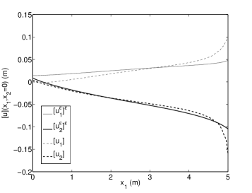
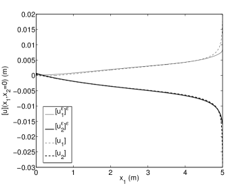
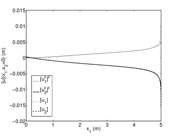
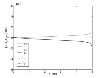
Figure 4: Exemple 1 – Jump in the displacement $[u](x_{1},x_{2}=0)$ (m) along the interface: $\varepsilon=0.1$ m (left top), $\varepsilon=0.01$ m (right top), $\varepsilon=0.005$ m (left bottom) and $\varepsilon=0.001$ m (right bottom)

We can observe that, as expected, when $\varepsilon=0.1$ m the difference between the jumps across the interphase and the jumps across the interface are relatively large (with a maximum relative error of about 30%). For smaller values of the thickness $\varepsilon$ of the interphase, the difference between the results obtained using the interphase problem and those obtained using the interface approximation is negligible. More precisely, the maximum relative error is close to 1% for $\varepsilon=0.01$ m, $0.6\%$ for $\varepsilon=0.005$ m and $0.2\%$ for $\varepsilon=0.001$ m.

4.2 Jump $[\sigma_{12}]$ across the interface

In this paragraph, we present a comparison between the traction amplitude $\sigma_{12}$ at the top of the interphase/interface and at the bottom of the interphase/interface computed for the original interphase problem and for the approximated (at order 1) problem with the interface. They are respectively referred as $\sigma^{up}$ and $\sigma^{bottom}$ on figures (5) to (7). In the comparison, the thickness $\varepsilon$ ranges from 0.01 m to 0.001 m. We also present the traction amplitude computed at order 0 for the approximated problem. Since the traction is continuous across the interface, i.e. $[\sigma_{12}]=0$, the traction amplitude takes the same value at the top and at the bottom of the interface.

The case $\varepsilon=0.1$ m is not presented here because the difference between the case with the interphase and the case with the interface is large.

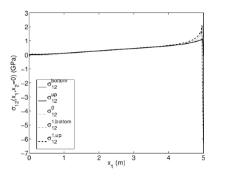
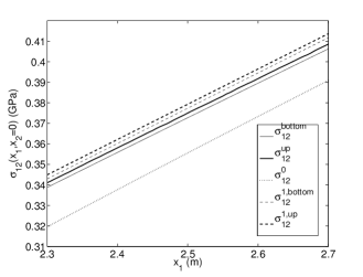
Figure 5: Exemple 1 ($\varepsilon=0.01$ m) – Stress $\sigma_{12}(x_{1},x_{2}=0)$ (GPa) at the bottom of the elastic adherent (up) and on the rigid base (bottom) computed with the various approximations (zoom on the right)

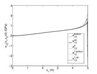
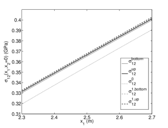
Figure 6: Exemple 1 ($\varepsilon=0.005$ m) – Stress $\sigma_{12}(x_{1},x_{2}=0)$ (GPa) at the bottom of the elastic adherent (up) and on the rigid base (bottom) computed with the various approximations (zoom on the right)

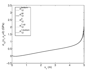
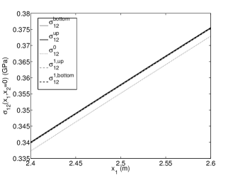
Figure 7: Exemple 1 ($\varepsilon=0.001$ m) – Stress $\sigma_{12}(x_{1},x_{2}=0)$ (GPa) at the bottom of the elastic adherent (up) and on the rigid base (bottom) computed with the various approximations (zoom on the right)

We can observe that the stress $\sigma_{12}$ computed using the interphase problem numerically converges to the stress $\sigma_{12}$ computed using the interface problem when $\varepsilon$ tends to 0.

One can also observe that the traction amplitude calculated at order 0 converges much slower than the traction amplitude calculated at order 1.

In conclusion, it seems that we can replace the interphase behavior by the interface law at order 1, for a thickness of glue lower than 0.01 m, i.e. less than 1% of the dimension of the structure.

4.3 Time computing

In this paragraph, we present the time computing necessary to obtain the solutions of the problems considered in the previous section.

Thickness	Number of	Number of	Number of	CPU time
$\varepsilon$ (m)	nodes	elements	degrees of freedom	(sec.)
$0.1$	2,582	4,966	4,962	6.4
$0.01$	28,172	55,166	54,342	48
$0.005$	39,486	77,432	76,304	66
$0.001$	150,054	294,831	290,106	274

Table 1: Mesh properties (T3 finite elements) and times computing for the interphase problem and various values of $\varepsilon$

Thickness	Number of	Number of	Number of	CPU time
$\varepsilon$ (m)	nodes	elements	degrees of freedom	(sec.)
$0.1$	731	1,363	1,410	5.2
$0.01$	10,887	5338	21,372	22
$0.005$	12,511	6,138	24,620	24
$0.001$	13,417	6,586	26,332	25

Table 2: Mesh properties (T6 finite elements) and times computing for the interface problem and various values of $\varepsilon$

Even if only linear finite elements are necessary for the computations for the interphase problem, we can notice that the CPU times necessary to obtain the solution quickly increases as the thickness of the interphase tends to 0. The reason is that the mesh has to be sufficiently fine inside the interphase, at least four nodes along the thickness. Therefore, in order to keep a reasonable condition number for the rigidity matrix, the mesh has to be fine also in a large zone around the interphase. This necessity significantly increases the number of degrees of freedom as the thickness of the interphase tends to zero.

For the interface problem, the computation is relatively independent of the parameter $\varepsilon$. As a consequence, the meshes and the CPU times of the computations increase very slowly as the thickness tends to zero. So, for small values of the thickness, the use of the imperfect interface model is very convenient.

5 Numerical results for two elastic bodies glued

In this section, we present examples of two elastic structures glued together. These examples are inspired by Goglio et al. (2008).

The first one is composed of two T-form elastic bodies (Aluminium) glued with an epoxy resin (see figure 8 for the geometry). More precisely, the mechanical coefficients of the materials are as follows:

• In the adhesive (Epoxy resin): $\hat{E}=4GPa$, $\hat{\nu}=0.33$.

• In the adherent (Aluminium): $E=70GPa$, $\nu=0.33$.

Figure 8: Exemple 2: geometry of the problem ($\varepsilon=0$ for the interface problem)

We present results for $\varepsilon=0.01$ m.

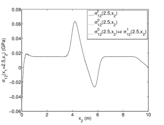
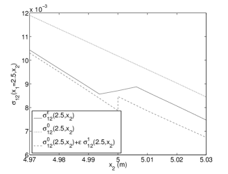
Figure 9: Exemple 2 ($\varepsilon=0.01$ m) – Stress $\sigma_{12}(x_{1}=2.5,x_{2})$ (GPa) on a vertical cut

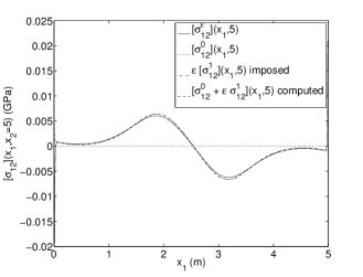
Figure 10: Exemple 2 ($\varepsilon=0.01$ m) – Jump in the stress $[\sigma_{12}](x_{1},x_{2}=5)$ (GPa) along the interface

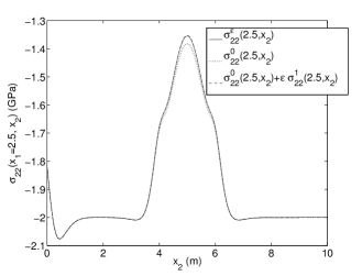
Figure 11: Exemple 2 ($\varepsilon=0.01$ m) – Stress $\sigma_{22}(x_{1}=2.5,x_{2})$ (GPa) on a vertical cut

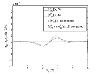
Figure 12: Exemple 2 ($\varepsilon=0.01$ m) – Jump in the stress $[\sigma_{22}](x_{1},x_{2}=5)$ (GPa) along the interface

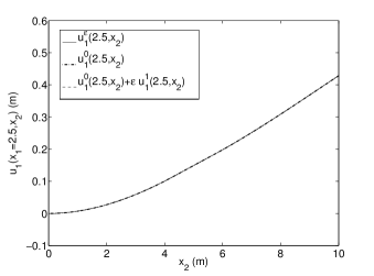
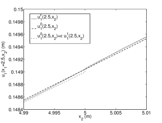
Figure 13: Exemple 2 ($\varepsilon=0.01$ m) – Displacement $u_{1}(x_{1}=2.5,x_{2})$ (m) on a vertical cut (Zoom on the right)

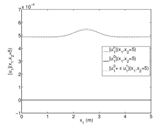
Figure 14: Exemple 2 ($\varepsilon=0.01$ m) – Jump in the displacement $[u_{1}](x_{1},x_{2}=5)$ (m) along the interface

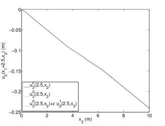
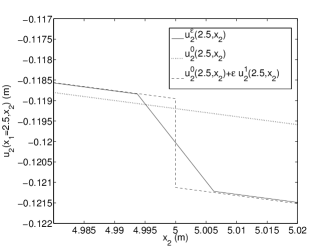
Figure 15: Exemple 2 ($\varepsilon=0.01$ m) – Displacement $u_{2}(x_{1}=2.5,x_{2})$ (m) on a vertical cut (Zoom on the right)

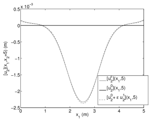
Figure 16: Exemple 2 ($\varepsilon=0.01$ m) – Jump in the displacement $[u_{2}](x_{1},x_{2}=5)$ (m) along the interface

The results show that the interface law at order 1 is able to reproduce the phenomena that occur in the interphase much more accurately that the interface law at order 0.

For example, we observe that $\sigma_{12}$ and the jump $[\sigma_{12}]$ are in good agreement with $\sigma^{\varepsilon}_{12}$ and $[\sigma^{\varepsilon}_{12}]$, respectively (see figures 9 and 10).

Even in the case of a small jump of a quantity (see figure 12 for $[\sigma_{22}]$, figure 14 for $[u_{1}]$), considering the order 1 term improve the results (see figure 11 for the stress $\sigma_{22}$ and figure 13 for displacement $u_{1}$).

Finally, the model is able to reproduce the displacement jump $[u_{2}]$ and the displacement $u_{2}$ with a very small error (see figure 15 and 16).

In our last example, we consider the same geometry as before. The materials are now as follows:

• The adhesive is a reinforced Epoxy resin: $\hat{E}=6GPa$, $\hat{\nu}=0.33$.

• The adherents are made of Polymethyl Methacrylate (PPMA) : ${E}=3.1GPa$, $\nu=0.4$.

In this last example, the elasticity coefficients of the components are very close. Let us observe that if they are identical, then the jumps conditions at order 0, that is to say $[u]=0$ and $[\sigma n]=0$, are exact conditions. This example permit us to observe the improvement provided by the first order terms in the case of a small mechanical properties variation between the glue and the adherents.

We present here only the results for the displacement $u_{2}$ (normal to the interface) and for the stress $\sigma_{22}$, because they are representative of the results for the other components.

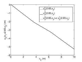
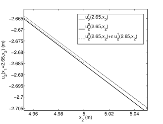
Figure 17: Exemple 3 ($\varepsilon=0.01$ m) – Displacement $u_{2}(x_{1}=2.65,x_{2})$ (m) on a vertical cut (Zoom on the right)

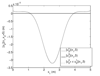
Figure 18: Exemple 3 ($\varepsilon=0.01$ m) – Jump in the displacement $[u_{2}](x_{1},x_{2}=5)$ (m) along the interface

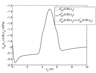
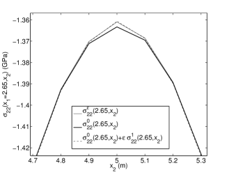
Figure 19: Exemple 3 ($\varepsilon=0.01$ m) – Stress $\sigma_{22}(x_{1}=2.65,x_{2})$ (GPa) on a vertical cut (Zoom on the right)

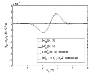
Figure 20: Exemple 3 ($\varepsilon=0.01$ m) – Jump in the stress $[\sigma_{22}](x_{1},x_{2}=5)$ (GPa) along the interface

Due to the small difference between the mechanical properties of the glue and the adherents, we can observe in figure 18 that the jump in the displacement is very small compared to the size of the structure (less than $2\cdot 10^{-3}\%$ of the size of the structure), and to the maximum of the displacement represented in figure 17 (less than $10^{-2}\%$ of the maximum of the displacement of the structure). Nevertheless, considering the first order term improves the asymptotic approximation of the displacement (see figure 17) and the stress (see figure 19). Moreover, the jump in the stress $[\sigma_{22}]$ is well approximated (see figure 20). The oscillations that we can observe in figure 20 are due to the smallness of the stress jump, that is of the same order of the error of the approximation.

6 Conclusion

In this paper, we have presented an interface law at order 1 when the Lamé’s coefficients of the adhesive do not rescale with the thickness of the interphase. Based on the proposed interface law, some numerical experiments were also presented that show the accuracy of the method when the interphase thickness becomes smaller and smaller. For this purpose, we have developed an original numerical scheme based on the Nitsche’s method to simulate the adhesion between two elastic materials.

This model is very efficient (maximum relative error less than 1 % for a ratio of thickness smaller than 1 %) and the interface law is able to reproduce the mechanical behavior of the real interface. On the other hand, the numerical model developed in this paper is less expensive than the solution of the real problem. More precisely, the method is independent of the thickness of the interphase and it becomes more and more efficient as the thickness decreases. For example, in the first numerical test proposed above, the CPU times of the interphase problem and the asymptotic interface problem are equivalent when $\varepsilon=0.1$, but their ratio is lower than $\frac{1}{10}$ when $\varepsilon=0.001$.

References

References

- Abdelmoula et al. (1998) Abdelmoula, R., Coutris, M., Marigo, J. J., 1998. Comportement asymptotique d’une interface mince. C. R. Acad. Sci. IIB 326 (4), 237–242.
-
Baiocchi et al. (1992)
Baiocchi, C., Brezzi, F., Marini, L., 1992. Stabilization of galerkin methods
and applications to domain decomposition. In: Bensoussan, A., Verjus, J.-P.
(Eds.), Future Tendencies in Computer Science, Control and Applied
Mathematics. Vol. 653 of Lecture Notes in Computer Science. Springer Berlin
Heidelberg, pp. 343–355.
URL http://dx.doi.org/10.1007/3-540-56320-2_71 - Barbosa and Hughes (1992) Barbosa, H. J. C., Hughes, T. J. R., 1992. Boundary lagrange multipliers in finite element methods: error analysis in natural norms. Numer. Math. 62 (1), 1–15.
- Becker et al. (2010) Becker, R., Hansbo, P., Stenberg, R., 2010. A finite element method for domain decomposition with non-matching grids. ESAIM: M2AN 37 (2), 209–225.
- Benveniste (2006) Benveniste, Y., 2006. An interface model of a three-dimensional curved interphase in conduction phenomena. Proc. R. Soc. A 462, 1593–1617.
- Bertoldi et al. (2007a) Bertoldi, K., Bigoni, D., Drugan, W., 2007a. Structural interfaces in linear elasticity. Part I: Nonlocality and gradient approximations. J. Mech. Phys. Solids 55 (1), 1–34.
- Bertoldi et al. (2007b) Bertoldi, K., Bigoni, D., Drugan, W., 2007b. Structural interfaces in linear elasticity. Part II: Effective properties and neutrality. J. Mech. Phys. Solids 55 (1), 35–63.
- Bigoni and Movchan (2002) Bigoni, D., Movchan, A., 2002. Statics and dynamics of structural interfaces in elasticity. Int. J. Solids Struct. 39, 4843–4865.
- Cognard et al. (2011) Cognard, J. Y., Bourgeois, M., Créac’hcadec, R., Sohier, L., 2011. Comparative study of the results of various experimental tests used for the analysis of the mechanical behaviour of an adhesive in a bonded joint. J. Adhes. Sci. Technol. 25 (20), 2857–2879.
- Cognard et al. (2006) Cognard, J. Y., Davies, P., Sohier, L., Créac’hcadec, R., 2006. A study of the non-linear behaviour of adhesively-bonded composite assemblies. Compos. Struct. 76, 34–46.
- Dumont et al. (2006) Dumont, S., Goubet, O., Ha-Duong, T., Villon, P., 2006. Meshfree methods and boundary conditions. Int. J. Numer. Meth. Engng. 67, 989–1011.
- Duong et al. (2011) Duong, V. A., Diaz, A. D., Chataigner, S., Caron, J.-F., 2011. A layerwise finite element for multilayers with imperfect interfaces. Compos. Struct. 93 (12), 3262–3271.
- Geuzaine and Remacle (2009) Geuzaine, C., Remacle, J.-F., 2009. Gmsh: a three-dimensional finite element mesh generator with built-in pre- and post-processing facilities. Int. J. Numer. Meth. Engng. 79 (11), 1309–1331.
- Goglio et al. (2008) Goglio, L., Rossetto, M., Dragoni, E., 2008. Design of adhesive joints based on peak elastic stresses. Int. J. Adhes. Adhes. 28 (8), 427–435.
- Hirschberge et al. (2009) Hirschberge, C. B., Ricker, S., Steinmann, P., Sukumar, N., 2009. Computational multiscale modelling of heterogeneous material layers. Eng. Fract. Mech. 767 (6), 793–812.
- Klarbring (1991) Klarbring, A., 1991. Derivation of the adhesively bonded joints by the asymptotic expansion method. Int. J. Eng. Sci. 29 (4), 493–512.
- Krasuki and Lenci (2000) Krasuki, F., Lenci, S., 2000. Yield design of bonded joints. Eur. J. Mech. A-Solid 19 (4), 649–667.
- Kumar and Mittal (2011) Kumar, M., Mittal, P. A., 2011. Methods for solving singular perturbation problems arising in science and engineering. Math. Comput. Model. 54 (1-2), 556–575.
- Kumar and Scanlan (2010) Kumar, S., Scanlan, J. P., 2010. Stress analysis of shaft-tube bonded joints using a variational method. J. Adhesion 86 (4), 369–394.
- Lebon et al. (1997) Lebon, F., Ould-Khaoua, A., Licht, C., 1997. Numerical study of soft adhesively bonded joints in finite elasticity. Comput. Mech. 21, 134–140.
- Lebon and Rizzoni (2008) Lebon, F., Rizzoni, R., 2008. Asymptotic study of a soft thin layer: the non convex case. Mech. Adv. Mat. Struct. 15 (1), 12–20.
- Lebon and Rizzoni (2010) Lebon, F., Rizzoni, R., 2010. Asymptotic analysis of a thin interface: The case involving similar rigidity. Int. J. Eng. Sci. 48 (5), 473–486.
- Lebon and Rizzoni (2011a) Lebon, F., Rizzoni, R., 2011a. Asymptotic behavior of a hard thin linear interphase: An energy approach. Int. J. Solids Struct. 48 (3-4), 441–449.
- Lebon and Rizzoni (2011b) Lebon, F., Rizzoni, R., 2011b. Modelling adhesion by asymptotic techniques. In: Wilkinson, K. A., Ordonez, D. A. (Eds.), Adhesive Properties in Nanomaterials, Composites and Films. Materials Science and Technologies. Nova Publisher, pp. 95–126.
- Lebon et al. (2004) Lebon, F., Rizzoni, R., Ronel-Idrissi, S., 2004. Analysis of non-linear soft thin interfaces. Comput. Struct. 82 (23-26), 1929–1938.
- Lebon and Ronel-Idrissi (2007) Lebon, F., Ronel-Idrissi, S., 2007. First-order numerical analysis of linear thin layer. J. Appl. Mech.-T. ASME 74, 824–828.
- Lebon and Zaittouni (2010) Lebon, F., Zaittouni, F., 2010. Asymptotic modelling of interface taking into account contact conditions: Asymptotic expansions and numerical implementation. Int. J. Eng. Sci. 48 (2), 111–127.
- Licht and Michaille (1997) Licht, C., Michaille, G., 1997. A modeling of elastic adhesive bonded joints. Adv. Math. Sci. Appl. 7, 711–740.
- Nguyen et al. (2012) Nguyen, D. T., D’Ottavio, M., Caron, J.-F., 2012. Benchmark of a layerwise stress model for laminated and sandwich plates [benchmark d’un modèle pour sandwiches et multicouches, de type layerwise en contrainte]. Annales de Chimie: Science des Matériaux 37 (2-4), 445–456.
- Nitsche (1974) Nitsche, J. A., 1974. Convergence of nonconforming methods(finite element solution for dirichlet problem). In: De Boor, C., of Wisconsin-Madison. Mathematics Research Center, U. (Eds.), Mathematical Aspects of Finite Elements in Partial Differential Equations: Proceedings of a Symposium Conducted by the Mathematics Research Center, the University of Wisconsin–Madison, April 1-3, 1974. Publication (The Mathematics Research Center. University of Wisconsin). Academic Press, pp. 15–53.
- Rizzoni and Lebon (2012) Rizzoni, R., Lebon, F., 2012. Asymptotic analysis of an elastic thin interphase with mismatch strain. Eur. J. Mech. A-Solid 36, 1–8.
- Sacco and Lebon (2012) Sacco, E., Lebon, F., 2012. A damage-friction interface model derived from micromechanical approach. Int. J. Solids Struct. 49 (26), 3666–3680.
- Sánchez-Palencia (1980) Sánchez-Palencia, E., 1980. Non-homogeneous media and vibration theory. Vol. 127 of Lect. Notes Phys. Springer-Verlag.
- Stenberg (1995) Stenberg, R., 1995. On some techniques for approximating boundary conditions in the finite element method. J. Comput. Appl. Math. 63 (1-3), 139–148.
- Zaittouni et al. (2002) Zaittouni, F., Lebon, F., Licht, C., 2002. Etude théorique et numérique du comportement d’un assemblage de plaques. C. R. Acad. Sci. II 330, 359–364.