Identifiable reparametrizations of linear compartment models

Abstract.

Structural identifiability concerns finding which unknown parameters of a model can be quantified from given input-output data. Many linear ODE models, used in systems biology and pharmacokinetics, are unidentifiable, which means that parameters can take on an infinite number of values and yet yield the same input-output data. We use commutative algebra and graph theory to study a particular class of unidentifiable models and find conditions to obtain identifiable scaling reparametrizations of these models. Our main result is that the existence of an identifiable scaling reparametrization is equivalent to the existence of a scaling reparametrization by monomial functions. We provide an algorithm for finding these reparametrizations when they exist and partial results beginning to classify graphs which possess an identifiable scaling reparametrization.

Keywords: Identifiability, Compartment models, Reparametrization

1. Introduction

Parameter identifiability analysis for dynamic system ODE models addresses the question of which unknown parameters can be quantified from given input-output data. This paper is concerned with structural identifiability analysis, that is whether the parameters of a model could be identified if perfect input-output data (noise-free and of any duration required) were available. If the parameters of a model have a unique or finite number of values given input-output data, then the model and its parameters are said to be identifiable. However, if some subset of the parameters can take on an infinite number of values and yet yield the same input-output data, then the model and this subset of parameters are called unidentifiable. In such cases, we attempt to reparametrize the model to render it identifiable.

There have been several methods proposed to find these identifiable reparametrizations. Evans and Chappell [8] use a Taylor Series approach, Chappell and Gunn [5] use a similarity transformation approach, and both Ben-Zvi et al [2] and Meshkat et al [12] use a differential algebra approach to find identifiable reparametrizations of nonlinear ODE models (see [14] for a survey of methods). However, as demonstrated in [8], there is no guarantee that these reparametrizations will be rational. For practical applications, e.g. in systems biology, a rational reparametrization is desirable. The motivation for this paper is to address the following question for linear systems:

Question 1.1.

For which linear ODE models does there exist a rational identifiable reparametrization?

In this paper, we focus on scaling reparametrizations, which are reparametrizations that are obtained by replacing an unobserved variable by a scaled version of itself, and updating the model coefficients accordingly. We will answer the above question and provide an algorithm (see Algorithm 6.1) which takes as its input a system of linear ODEs with parametric coefficients and gives as its output an identifiable scaling reparametrization, if it exists, or shows that no identifiable scaling reparametrization exists.

Our main result gives a precise characterization of when a scaling reparametrization exists, for a specific family of linear ODE models.

Theorem 1.2.

Consider the linear compartment model with associated strongly connected graph $G$, where the input and output are in the same compartment. The following conditions are equivalent for this model:

1. The model has an identifiable scaling reparametrization.

2. The model has an identifiable scaling reparametrization by monomial functions of the original parameters.

3. The dimension of the image of the double characteristic polynomial map associated to $G$ is equal to the number of linearly independent cycles in $G$.

Note the two key features of the theorem: by part (2) we only need to consider monomial scaling reparametrizations of the model, and by part (3) checking for the existence of an identifiable monomial rescaling is equivalent to determining the dimension of the image of a certain algebraic map, the double characteristic polynomial map. Theorem 1.2 leaves open the problem of characterizing the graphs $G$ which satisfy the necessary dimension requirements, but we provide a number of partial results, including upper bounds on the number of edges that can appear, and constructions of families of graphs which realize the dimension bound, and hence have identifiable reparametrizations by monomial rescalings.

The organization of the paper is as follows. The next section provides introductory material on compartment models, how to derive the input-output equation, identifiability, and reparametrizations. Section 2 also introduces the main algebraic object of study in this paper: the double characteristic polynomial map. Section 3 explains how the identifiability problem relates to the directed cycles in the graph $G$, and how the cycle structure gives bounds on the dimension of the image of the double characteristic polynomial map. Section 4 contains a proof of Theorem 1.2, which reduces the problem of characterizing the graphs which have a scaling reparametrization to the problem of calculating the dimension of the image of the double characteristic polynomial map. Section 5 includes various combinatorial constructions to achieve the correct dimension, as well as some necessary conditions. In particular, we show that all minimal inductively strongly connected graphs achieve the correct dimension, and hence have an identifiable scaling reparametrization. Section 6 summarizes our theoretical results with an algorithm for computing an identifiable scaling reparametrization (if one exists). Section 6 also includes the results of systematic computations for graphs with few vertices, and contains conjectures based on the results of those computations.

2. Identifiability and Reparametrizations

Let $G$ be a directed graph with $m$ edges and $n$ vertices. We associate a matrix $A(G)$ to the graph in the following way:

$$A(G)_{ij}=\left\{\begin{array}[]{l l l}a_{ii}&\quad\text{if $i=j$}\\ a_{ij}&\quad\text{if $j\rightarrow{i}$ is an edge of $G$}\\ 0&\quad\text{otherwise,}\\ \end{array}\right.$$

where each $a_{ij}$ is an independent real parameter. For brevity, we will use $A$ to denote $A(G)$.

Consider the ODE system of the form,

(1) $$\dot{x}(t)=Ax(t)+u(t)\ \ \ \ \ \ \ \ y=x_{1}$$

where $x(t)\in\mathbb{R}^{n}$ and $u(t)\in\mathbb{R}^{n}$, with $u(t)={\begin{pmatrix}u_{1}(t)&0&\ldots&0\end{pmatrix}}^{T}$.

Such models are called linear compartment models [4], where $x$ is the state variable, $u$ is the input vector, $y$ is the output, and the nonzero entries $a_{ij}$ of $A$ are independent parameters. Since $G$ is a directed graph with $m$ edges and $n$ vertices, the dimension of the parameter space of this model is $m+n$. Note that $u$ has only one nonzero entry in the first coordinate, and that our output is $y=x_{1}$, which is also from the first compartment. Hence, in this paper we only consider models where there is a single input and output and both are in the same compartment. Note that we can only observe the input $u_{1}$ and the output $y$: the state variable $x$ and the parameter entries of $A$ are unknown.

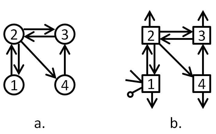
Figure 1. a.) A graph with four vertices and b.) A compartment model

Example 2.1.

For the directed graph $G$ on four vertices with six edges in Figure 1a, the ODE system has the following form:

$$\begin{pmatrix}\dot{x}_{1}\\ \dot{x}_{2}\\ \dot{x}_{3}\\ \dot{x}_{4}\end{pmatrix}={\begin{pmatrix}a_{11}&a_{12}&0&0\\ a_{21}&a_{22}&a_{23}&0\\ 0&a_{32}&a_{33}&a_{34}\\ 0&a_{42}&0&a_{44}\end{pmatrix}}{\begin{pmatrix}x_{1}\\ x_{2}\\ x_{3}\\ x_{4}\end{pmatrix}}+{\begin{pmatrix}u_{1}\\ 0\\ 0\\ 0\end{pmatrix}}$$

$$y=x_{1}.$$

From a biological perspective, we think of the vertices as compartments and the unknown parameters as exchange rates between the compartments. The off-diagonal entries $a_{ij}$ of $A$ are the instantaneous rates of transfer of material from the $j$th compartment to the $i$th compartment. If there is no edge $j\to i$, then then is no direct transfer of material from compartment $j$ to compartment $i$. In addition, each compartment is assumed to have a leak, i.e. an outflow of material from that compartment outside the system. In a typical biological setup, the diagonal entries $a_{ii}$ are expressed as the negative sum of the leak, written as $a_{0i}$, and the other entries in the $i$th column, so that $a_{ii}=-a_{0i}-\sum_{j\neq{i}}{a_{ji}}$. Hence, for biological applications, we would assume that our matrix $A(G)$ has nonnegative off-diagonal entries, negative diagonal entries, and with the leak assumption, it will be strictly diagonally dominant.

In a typical setup from a biological application, the graph from Example 2.1 would have the compartment model representation in Figure 1b. The square vertices represent compartments, outgoing arrows from each compartment represent leaks, the edge with a circle coming out of compartment $1$ represents the output, and the arrowhead pointing into compartment $1$ represents the input. However, since we will have a leak at every compartment, and always have the input and output in the same compartments, we will not draw these features in our graphs throughout the paper.

Since we can only observe the input and output to the system, we are interested in relating these quantities by forming an input-output equation, i.e. an equation purely in terms of input, output, and parameters. We will use the input-output equation to address the problem of identifiability of the model parameters, although there are other methods to do so, as demonstrated in [14]. There have been several methods proposed to find the input-output equations of nonlinear ODE models [11, 13], but for linear models the problem is much simpler.

Theorem 2.2.

Let $A_{1}$ be the submatrix of $A$ obtained by deleting the first row and column of $A$. Let $\tilde{f}$ be the characteristic polynomial of $A$, $\tilde{f}_{1}$ the characteristic polynomial of $A_{1}$, $g=\gcd(\tilde{f},\tilde{f}_{1})$, $f=\tilde{f}/g$ and $f_{1}=\tilde{f}_{1}/g$. Then the input-output equation of the system (1) is

$$f(\textstyle\frac{d}{dt})y=f_{1}(\textstyle\frac{d}{dt})u_{1}.$$

In particular, if the characteristic polynomials of $A$ and $A_{1}$ are relatively prime then, the input-output equation of the system (1) is

(2) $$y^{(n)}+c_{1}y^{(n-1)}+\cdots+c_{n}y=u_{1}^{(n-1)}+d_{1}u_{1}^{(n-2)}+\cdots+d_{n-1}u_{1}$$

where $c_{1},\ldots,c_{n}$ are the coefficients of the characteristic polynomial of $A$ and $d_{1},\ldots,d_{n-1}$ are the coefficients of the characteristic polynomial of $A_{1}$.

Proof.

We can re-write our ODE system as:

$$(\partial{I}-A)x=u$$

where $\partial$ is the differential operator $d/dt$. Using formal manipulations with this operator, we can use Cramer’s Rule to get that

$$x_{1}=det(A_{2})/det(\partial{I}-A)$$

where $A_{2}$ is the matrix $(\partial{I}-A)$ with the first column replaced by $u$. Since $u$ has $u_{1}$ as its first entry and zeros otherwise, then $det(A_{2})$ can be simplified as $det(\partial{I}-A_{1})u_{1}$, where $A_{1}$ is the submatrix of $A$ where the first row and first column have been deleted. Then replacing $x_{1}$ with $y$, we get the input-output equation:

$$det(\partial{I}-A)y=det(\partial{I}-A_{1})u_{1}.$$

In other words, $\tilde{f}(\frac{d}{dt})y=\tilde{f}_{1}(\frac{d}{dt})u_{1}$. Dividing both sides by $g=\gcd(\tilde{f},\tilde{f}_{1})$, we get $f(\frac{d}{dt})y=f_{1}(\frac{d}{dt})u_{1}$.

If $g=1$, we have that the input-output equation is of the form:

$$y^{(n)}+c_{1}y^{(n-1)}+\ldots+c_{n}y=u_{1}^{(n-1)}+d_{1}u_{1}^{(n-2)}+\ldots+d_{n-1}u_{1}$$

where the coefficients $c_{1},\ldots,c_{n}$ are the $n$ coefficients of the characteristic polynomial of $A$ and the coefficients $d_{1},\ldots,d_{n-1}$ are the $n-1$ coefficients of the characteristic polynomial of $A_{1}$. ∎

Remark.

We will show in Section 3 that the input-output equation has the form (2) for generic choices of the parameters $A$ if and only if $G$ is strongly connected.

Example 2.3.

For the graph in Example 2.1, the input-output equation is:

$$y^{(4)}-E_{1}(a_{11},a_{22},a_{33},a_{44})y^{(3)}+(E_{2}(a_{11},a_{22},a_{33},a_{44})-a_{12}a_{21}-a_{23}a_{32})y^{(2)}$$

$$-(E_{3}(a_{11},a_{22},a_{33},a_{44})-a_{11}a_{23}a_{32}-a_{12}a_{21}a_{33}+a_{23}a_{34}a_{42}-a_{12}a_{21}a_{44}-a_{23}a_{32}a_{44})y^{{}^{\prime}}$$

$$+(E_{4}(a_{11},a_{22},a_{33},a_{44})+a_{11}a_{23}a_{34}a_{42}-a_{11}a_{23}a_{32}a_{44}-a_{12}a_{21}a_{33}a_{44})y$$

$$=\quad\quad u_{1}^{(3)}-E_{1}(a_{22},a_{33},a_{44})u_{1}^{(2)}+(E_{2}(a_{22},a_{33},a_{44})-a_{23}a_{32})u_{1}^{{}^{\prime}}$$

$$-(E_{3}(a_{22},a_{33},a_{44})+a_{23}a_{34}a_{42}-a_{23}a_{32}a_{44})u_{1}$$

where $E_{k}(z_{1},\ldots,z_{m})$ denotes the $k$-th elementary symmetric polynomial in $z_{1},\ldots,z_{m}$.

Identifiability of an input-output equation concerns whether it is possible to recover the parameters of the model (in our case, the entries of $A$) only observing the relations among the input and output variables. In other words, we assume that we observe specific values of the coefficients $c_{1},\ldots,c_{n}$ and $d_{1},\ldots,d_{n-1}$ and we ask whether it is possible to recover the entries of $A$. More generally, we can ask for functions of the parameters $A$ which can be computed from $c_{1},\ldots,c_{n}$ and $d_{1},\ldots,d_{n-1}$. Such a function is called an identifiable function. We make these notions precise in generality.

Definition 2.4.

Let $c$ be a function $c:\Theta\rightarrow{\mathbb{K}^{m_{2}}}$, where $\Theta\subseteq\mathbb{K}^{m_{1}}$ and $\mathbb{K}$ is a field. The model parameters in $\Theta$ are globally identifiable from $c$ if and only if the map $c$ is injective. A subset of the model parameters in $\Theta$ are locally identifiable from $c$ if and only if the map $c$ is finite-to-one. A subset of the model parameters in $\Theta$ are unidentifiable from $c$ if and only if the map $c$ is infinite-to-one.

It is often the case that parameters might fail to be identifiable, but only on a small subset of parameter space. In this case, we can say that identifiability holds generically. For example, the model parameters in $\Theta$ are generically globally identifiable from $c$ if there is a dense open subset $U$ of $\Theta$, such that $c:U\rightarrow\mathbb{K}^{m_{2}}$ is globally identifiable. Similarly, we can define generically locally identifiable, and generically unidentifiable.

Remark.

For brevity, we make the convention for the remainder of the paper that identifiable means generically locally identifiable and unidentifiable means generically unidentifiable.

We can also speak of identifiability of individual functions.

Definition 2.5.

Let $c$ be a function $c:\Theta\rightarrow{\mathbb{K}^{m_{2}}}$, where $\Theta\subseteq\mathbb{K}^{m_{1}}$ and $\mathbb{K}$ is a field. A function $f:\Theta\rightarrow\mathbb{K}$ is globally identifiable from $c$ if there exists a function $\Phi:\mathbb{K}^{m_{2}}\rightarrow\mathbb{K}$ such that $\Phi\circ c=f$. The function $f$ is locally identifiable if there is a finitely multivalued function $\Phi:\mathbb{K}^{m_{2}}\rightarrow\mathbb{K}$ such that $\Phi\circ c=f$.

Similarly, we can define generic identifiability of a function. For brevity, for the remainder of the paper, when we say that a function is identifiable, we will mean that it is generically locally identifiable.

Proposition 2.6.

Suppose that $\Theta$ is a full dimensional subset of $\mathbb{K}^{m_{1}}$ and $c$ is a rational map. Then the model is identifiable from $c$ if and only if the dimension of the image of $c$ is $m_{1}$.

Also:

Proposition 2.7.

Suppose that $\Theta$ is a full dimensional subset of $\mathbb{K}^{m_{1}}$ and $c$ is a rational map, and $f:\Theta\rightarrow\mathbb{K}$ is a function. Then $f$ is identifiable if and only if

$$\mathbb{K}(f,c_{1},\ldots,c_{m_{1}})/\mathbb{K}(c_{1},\ldots,c_{m_{1}})$$

is a finite degree field extension.

Identifiability of the map $c$ or a function $f$ can be tested in specific instances using Gröbner basis calculations. See e.g. [9, 12].

In the setting of linear compartment models, we have a graph $G$ with $n$ vertices and $m$ directed edges. The parameter space $\Theta\subseteq\mathbb{R}^{m+n}$ consists of those matrices whose zero pattern is induced by the graph $G$, positive off-diagonal entries, negative diagonal entries, and strictly diagonally dominant. The map $c:\Theta\rightarrow\mathbb{R}^{2n-1}$ is the map that takes a matrix $A\in\Theta$ to the vector

$$(c_{1}(A),\ldots,c_{n}(A),d_{1}(A),\ldots,d_{n-1}(A))$$

of characteristic polynomial coefficients. The map $c:\Theta\rightarrow\mathbb{R}^{2n-1}$ is called the double characteristic polynomial map.

Example 2.8.

For the graph in Example 2.1, the image of the double characteristic polynomial map has dimension seven. A set of seven algebraically independent identifiable functions is $\left\{a_{11},\>a_{22},\>a_{33},\>a_{44},\>a_{12}a_{21},\>a_{23}a_{32},\>a_{23}a_{34}a_{42}\right\}$. For example, $a_{12}a_{21}$ is identifiable since, for this graph

$$a_{12}a_{21}=d_{2}-c_{2}+c_{1}d_{1}-d_{1}^{2}.$$

It is easy to see that these functions are algebraically independent (each involves a new indeterminate). The fact that they are identifiable follows from the material in Sections 3, 4, and 5.

The linear compartment models that we focus on in the present paper (that is, where the diagonal of $A$ contains algebraically independent parameters, or equivalently, every compartment has a leak) are never identifiable, except in the trivial case of a graph with one vertex. This will be explained in detail in the subsequent sections. This, however, forces us to look for identifiable reparametrizations of our model.

Definition 2.9.

A reparametrization of the input-output equation of a model is a map $q:\mathbb{R}^{m_{3}}\rightarrow\mathbb{R}^{m_{1}}$ such that the image of $c\circ q$ equals the image of $c$. The reparametrization is identifiable if the composed map $c\circ q$ is identifiable.

Since the new parametrization is $c\circ q$, there must exist a map $\Phi:{\rm im}\,c\rightarrow\mathbb{R}^{m_{3}}$ which is the (local) inverse of $c\circ q$. Since $q$ must be locally injective, this implies that the map $\Phi$ consists of identifiable functions of the map $c$. This argument is also reversible (e.g. by the implicit function theorem). Hence, finding an identifiable reparametrization is, from a theoretical standpoint, equivalent to finding $d$ algebraically independent functions $f_{1},\ldots,f_{d}$ that are identifiable from $c$, where $d=\dim{\rm im}\,c$. Once these identifiable functions $f$ are found, the goal is to determine a reparametrization of our original model that yields an input-output equation with coefficients $c\circ q$. In summary:

Proposition 2.10.

A reparametrization $q:\mathbb{R}^{m_{3}}\rightarrow\mathbb{R}^{m_{1}}$ of $c:\mathbb{R}^{m_{1}}\rightarrow\mathbb{R}^{m_{2}}$ is identifiable if and only if there is a map $\Phi:{\rm im}\,c\rightarrow\mathbb{R}^{m_{3}}$ such that $\Phi\circ c=f$ consists of identifiable functions from $c$.

A more subtle, and not quite mathematical, issue is that we want our reparametrization to both involve only relatively simple functions, and have an intuitively simple connection to our original model, without dramatic shifts in the parametrization. A common way to find such a reparametrization is via a rational scaling of the state variables [5, 8, 12], while other methods, e.g. affine maps of the state variables, can also be employed [7]. A scaling reparametrization is preferred over a more complicated type of reparametrization since it respects the biological properties of the original model. As we will see, when identifiable rescalings exist, they can always be made rational. For example, we would like to find a scaling:

$$X_{i}=f_{i}(A)x_{i}$$

such that the reparametrized model is identifiable, i.e. purely in terms of a fewer number of identifiable functions of parameters. Since $y=x_{1}$ is observed, we require that $f_{1}(A)=1$. In this way, the input and output variables remain intact. Scaling reparametrizations have the effect of nondimensionalizing the quantities that are being rescaled. That is, from input-output data we would not be able to estimate the values of those unobserved variables, but we can predict how their relative size changes as we change parameters.

The rescaling induced by the functions $f_{1},\ldots,f_{n}$ maps the matrix $A$ to $DAD^{-1}$, where $D=Diag(f_{i}(A))$. In other words, the entries of $A$ become:

$$a_{ij}\mapsto{a_{ij}f_{i}(A)/f_{j}(A)}$$

For this reparametrization to be identifiable, this means that the new coefficients of the state variables,

$$a_{ij}f_{i}(A)/f_{j}(A)$$

are themselves functions of identifiable functions of parameters by Proposition 2.10.

Example 2.11.

From the graph in Example 2.1, a possible rescaling is $X_{1}=x_{1},X_{2}=a_{12}x_{2},X_{3}=a_{12}a_{23}x_{3},X_{4}=a_{12}a_{23}a_{34}x_{4}$. This yields the reparametrized system:

$$\begin{pmatrix}\dot{X}_{1}\\ \dot{X}_{2}\\ \dot{X}_{3}\\ \dot{X}_{4}\end{pmatrix}={\begin{pmatrix}a_{11}&1&0&0\\ a_{12}a_{21}&a_{22}&1&0\\ 0&a_{23}a_{32}&a_{33}&1\\ 0&a_{23}a_{34}a_{42}&0&a_{44}\end{pmatrix}}{\begin{pmatrix}X_{1}\\ X_{2}\\ X_{3}\\ X_{4}\end{pmatrix}}+{\begin{pmatrix}u_{1}\\ 0\\ 0\\ 0\end{pmatrix}}$$

$$y=X_{1},$$

which is identifiable since each coefficient is a function of the seven identifiable functions from Example 2.8. We will see in Section 4 exactly how this reparametrization can be found.

Let $r:\mathbb{R}^{n+m}\rightarrow\mathbb{R}^{n+m}$ be the rescaling map associated to the functions $f_{i}$:

$$r_{ij}(A)=a_{ij}f_{i}(A)/f_{j}(A).$$

Proposition 2.12.

The dimension of the image of the rescaling map $r$ is greater than or equal to $\dim\Theta-(n-1)$.

Proof.

We can calculate this by finding the Jacobian. To simplify the calculation we first take the logarithm and call this function $\varphi_{ij}$:

$$\varphi_{ij}=log(f_{i}(A))-log(f_{j}(A))+log(a_{ij})$$

Then the derivative is:

$$\frac{\partial{\varphi_{ij}}}{\partial{a_{kl}}}=\frac{1}{f_{i}(A)}\frac{\partial{f_{i}(A)}}{\partial{a_{kl}}}-\frac{1}{f_{j}(A)}\frac{\partial{f_{j}(A)}}{\partial{a_{kl}}}+\delta_{kl,ij}\frac{1}{a_{ij}}$$

Thus, the Jacobian $J(\varphi)$ can be written as:

$$Diag(\frac{1}{a_{ij}})+J(a_{ij}\mapsto{log(f_{i}(A))})\cdot E(G)$$

where $J(a_{ij}\mapsto{log(f_{i}(A))})$ is the Jacobian of the mapping $a_{ij}\mapsto{log(f_{i}(A))}$ and $E(G)$ is the $n$ by $m$ incidence matrix (defined in Section 3, see Eq (3)). We can write this in shorthand notation as:

$$J(\varphi)=D+J\cdot E(G)$$

Then we have that $rank(J(\varphi))\geq{rank(D)-rank(J\cdot E(G))}$. From Proposition 3.8, we have that ${\rm rank}(E(G))\leq n-1$, which implies ${\rm rank}(J\cdot E(G))\leq n-1$, and thus:

$${\rm rank}(J(\varphi))\geq m+n-(n-1)=m+1$$

In other words, the dimension drops by at most $n-1$. ∎

This theorem gives us the maximal number of parameters of a model with an identifiable scaling reparametrization.

Corollary 2.13.

Let $G$ be a graph for which an identifiable scaling reparametrization of the system (1) exists. Then $G$ has at most $2n-2$ edges.

Proof.

Proposition 2.12 gives us the minimal dimension of the image of $r$, which is $\dim\Theta-(n-1)=m+1$. The dimension of the image of $c$ is at most $2n-1$. Since an identifiable reparametrization means that the dimension of the image of $c\circ q$ is the dimension of the image of $c$, the dimension of the image of $r$ must be at most $2n-1$. Thus $m$ is at most $2n-2$. ∎

This leads us to the main problem to be studied in the remainder of the paper:

Problem 2.14.

For which graphs $G$ with $n$ vertices and $\leq 2n-2$ edges does there exist a generically locally identifiable scaling reparameterization of the system (1) associated to the graph $G$?

Since local identifiability is completely determined by dimension, we can break the problem into three parts:

1. Determine the dimension $d$ of the image of the double characteristic polynomial map $c$ as a function of the graph $G$.

2. Find a set of $d$ algebraically independent identifiable functions from $c$.

3. Find an identifiable reparametrization of the ODE system, using the $d$ algebraically independent functions.

It is these three problems which we address in the subsequent sections.

3. Cycles and Monomials

In this section, we begin to relate the study of Problem 2.14 to the particular structure of the graph $G$. The cycles in $G$ play a crucial role, because of their appearance in the calculation of the characteristic polynomial. This section describes this relationship and relates the structure of cycles in the graph to the problem of finding identifiable reparametrizations. The connection between the cycle structure in the graph $G$ and identifiability of the associated linear compartment model has been employed in other works (see [1, 10]). However, our paper appears to be the first to use this structure to study the existence of identifiable reparametrizations.

Definition 3.1.

A closed path in a directed graph $G$ is a sequence of vertices $i_{0},i_{1},i_{2},\ldots,i_{k}$ with $i_{k}=i_{0}$ and such that $i_{j}\to i_{j+1}$ is an edge for all $j=0,\ldots,k-1$. A cycle in $G$ is a closed path with no repeated vertices. To a cycle $C=i_{0},i_{1},i_{2},\ldots,i_{k}$, we associate the monomial $a^{C}=a_{i_{1}i_{2}}a_{i_{2}i_{3}}\cdots a_{i_{k}i_{1}}$, which we refer to as a monomial cycle.

Note that the diagonals of $A$ are monomial $1$-cycles from the graph $G$.

Theorem 3.2.

The coefficients $c_{i}$ of the characteristic polynomial $\lambda^{n}+\sum_{i=1}^{n}{c_{i}\lambda^{n-i}}$ of $A$ are polynomial functions in terms of the monomial cycles, $a^{C}=a_{i_{1}i_{2}}a_{i_{2}i_{3}}\cdots a_{i_{k}i_{1}}$, of the graph $G$.

Specifically, let $\mathcal{C}(G)$ be the set of all cycles in $G$. Then

$$c_{i}=(-1)^{i}\sum_{C_{1},\ldots,C_{k}\in\mathcal{C}(G)}\prod_{j=1}^{k}{\rm sign}(C_{j})a^{C_{j}},$$

where the sum is over all collections of vertex disjoint cycles involving exactly $i$ edges of $G$, and ${\rm sign}(C)=1$ if $C$ is odd length and ${\rm sign}(C)=-1$ if $C$ is even length.

This follows from the expansion of the determinant, and breaking each permutation into its disjoint cycle decomposition.

Example 3.3.

Looking at the input-output equation for the graph from Example 2.1, which appears in Example 2.3, we see that the coefficient of $y^{\prime}$ is

$$-(E_{3}(a_{11},a_{22},a_{33},a_{44})-a_{11}a_{23}a_{32}-a_{12}a_{21}a_{33}-a_{12}a_{21}a_{44}-a_{23}a_{32}a_{44}+a_{23}a_{34}a_{42}).$$

The elementary symmetric function gives all terms that come from products of three $1$-cycles. All the terms with a minus sign come from products of a $2$-cycle and a $1$ cycle, and the final term comes from the single $3$-cycle in the graph.

Definition 3.4.

A graph $G$ is strongly connected if there is a directed path from any vertex to any other vertex. Equivalently, $G$ is strongly connected if the graph is connected and every edge belongs to a cycle.

Proposition 3.5.

Let $G$ be a graph, $A=A(G)$ be the associated matrix of indeterminates, and $A_{1}$ be the submatrix of $A$ obtained by deleting the first row and column of $A$. Let $f$ and $f_{1}$ be the characteristic polynomials of $A$ and $A_{1}$ respectively. Then $f$ and $f_{1}$ have a common factor if and only if $G$ is not strongly connected.

Proof.

If $G$ is not strongly connected after rearranging rows and columns of $A$, it will be a block upper triangular matrix. The characteristic polynomial of $A$ factors as the product of the characteristic polynomials of the diagonal blocks. The characteristic polynomial of $A_{1}$ will contain as factors, all of the factors for diagonal blocks of $A$ that do not involve row/column $1$.

On the other hand, if $G$ is strongly connected, the characteristic polynomial of $A$ is irreducible in the polynomial ring $\mathbb{K}(A)[\lambda]$, where $\mathbb{K}(A)$ is the fraction field in the entries of $A$. This can be seen by looking at the constant term of the characteristic polynomial, i.e. $\det(A)$, which itself is irreducible in the polynomial ring $\mathbb{K}[A]$. Indeed, if $\det(A)$ was reducible, we could partition in the vertices of $G$ into two disjoint sets such that there were no cycles passing between those sets of vertices. This contradicts the fact that $G$ is strongly connected. ∎

Remark.

If $G$ is a general graph with generic parameters, then the input-output equation will result from taking the largest strongly connected subgraph of $G$ that contains the vertex $1$. With this in mind, we will focus in the remainder of the paper only on strongly connected graphs.

Let $\mathcal{C}=\mathcal{C}(G)$ be the set of all directed cycles in the graph $G$. To each cycle $C=(i_{0},\ldots,i_{k})\in\mathcal{C}$ we associate the monomial cycle $a^{C}:=a_{i_{1}i_{2}}a_{i_{2}i_{3}}\cdots a_{i_{k}i_{1}}$. Define the cycle map by

$$\pi:\mathbb{R}^{m+n}\rightarrow\mathbb{R}^{\#\mathcal{C}},\quad A\mapsto(a^{C})_{C\in\mathcal{C}}.$$

Since the coefficients of the characteristic polynomial of $A$ and $A_{1}$ are both polynomials in terms of the cycles of $G$, the double characteristic polynomial map $c$ factors through the cycle map. That is, there is a polynomial map $\phi:\mathbb{R}^{\#\mathcal{C}}\rightarrow\mathbb{R}^{2n-1}$ such that $c=\phi\circ\pi$. As a consequence, we have the following proposition.

Proposition 3.6.

Let $G$ be a graph with $n$ vertices and $m$ edges. The dimension of the image of the double characteristic polynomial map $c$ is less than or equal to the dimension of the image of the cycle map $\pi$. In particular, $\dim{\rm im}\,c$ is bounded above by the number of algebraically independent monomial cycles in $G$.

Since the cycle map is a monomial map, it is easy to use linear algebra to calculate the dimension of its image. This is part of the connection between lattice polytopes and toric varieties [6], though we will not require advanced material from that theory. The main result for our story is the following.

Theorem 3.7.

Let $G$ be a strongly connected graph with $n$ vertices and $m$ edges. Then the dimension of the image of the cycle map $\pi$ is $m+1$.

We will phrase the proof of Theorem 3.7 in terms of the directed incidence matrix, a tool we will also need later in the paper. Let $G$ have $n$ vertices, $V=\left\{1,2,\ldots,n\right\}$, and $m$ directed edges. We can form the $n$ by $m$ directed incidence matrix $E(G)$, where

(3) $$E(G)_{i,(j,k)}=\left\{\begin{array}[]{l l l}1&\quad\text{if $i=j$}\\ -1&\quad\text{if $i=k$}\\ 0&\quad\text{otherwise.}\\ \end{array}\right.$$

In other words, $E(G)$ has column vectors $e_{jk}$ corresponding to the edges $j\rightarrow{k}$ with $1$ in the $jth$ row, $-1$ in the $kth$ row, and $0$ otherwise. Note that a $0/1$ vector in the kernel of $E(G)$ is the indicator vector of the disjoint union of a collection of cycles in $G$.

The rank of the directed incidence matrix is well-known (e.g. [3, Prop. 4.3]).

Proposition 3.8.

Let $G$ be a graph with $n$ vertices, $m$ edges, and $l$ connected components. Then the rank of $E(G)$ is $n-l$. Thus, the dimension of $\ker E(G)$ is $m-n+l$.

Proof of Theorem 3.7.

If $\phi:\mathbb{R}^{k_{1}}\rightarrow\mathbb{R}^{k_{2}}$ is a monomial map, the dimension of the image of $\phi$ is equal to the rank of the matrix whose columns are the monomials appearing in $\phi$. In the case of the cycle map, we should thus make a $0/1$ matrix $B$ whose columns are the cycles in $G$, and compute the rank of that matrix. All the one cycles, $(i,i)$, corresponding to the monomial $a_{ii}$ contribute one dimension to the rank of $B$, and those one cycles do not appear in any other cycles. Hence we can reduce to a matrix $B^{\prime}$ which eliminates those $n$ columns.

Thus, we are left with the $0/1$ matrix whose columns are the indicator vectors of all cycles in $G$. The columns of $B^{\prime}$ are all in the kernel of $E(G)$ (see e.g. [3, Theorem  4.5]). Since $G$ is strongly connected, $\dim\ker E(G)=m-n+1$. Hence, it suffices to show that the columns of $B^{\prime}$ generate the kernel of $E(G)$ when $G$ is strongly connected.

Let $v$ be an integer vector in the kernel of $E(G)$. Since $G$ is strongly connected, for each negative entry of $v$, there is a cycle $C$ passing through the corresponding edge of $G$. Let $1_{C}$ be the corresponding integer vector. Then for some large integer $k$, $v+k\cdot 1_{C}$ has decreased the number of negative entries of $v$. Continuing in this fashion, we can assume that $v$ has no negative entries.

A nonnegative integer vector $v$ such that $E(G)v=0$ corresponds to a multigraph (with edge $i\to j$ repeated $v_{ij}$ times) which has the property that the indegree of each vertex equals the outdegree. In such an Eulerian graph, we can start with any edge and walk around until closing off a cycle. Removing that cycle results in a smaller graph with the same property. This process expresses $v$ as a nonnegative integer combination of the indicator vectors of cycles. This completes the proof. ∎

Corollary 2.13 states that if $G$ is to have an identifiable scaling reparametrization, $G$ must have at most $2n-2$ edges. Theorem 3.7 and Proposition 3.6 say that this bound on the number of edges is at least compatible with the existence of an identifiable scaling reparametrization. We will address this issue in the next section.

4. Monomial Scaling Reparametrizations

The goal of this section is to prove Theorem 1.2, which we restate here for simplicity.

Theorem 1.2.

Consider the linear compartment model with associated strongly connected graph $G$, where the input and output are in the same compartment. The following conditions are equivalent for this model:

1. The model has an identifiable scaling reparametrization.

2. The model has an identifiable scaling reparametrization by monomial functions of the original parameters.

3. The dimension of the image of the double characteristic polynomial map associated to $G$ is equal to the number of linearly independent cycles in $G$.

Proof.

Clearly $(2)\implies(1)$. Also, it is not difficult to see that $(1)\implies(3)$. Indeed, if $G$ has $n$ vertices and $m$ edges, the dimension of the image of the double characteristic polynomial map is $\leq m+1$, $m+1$ being the number of linearly independent cycles in $G$ by Proposition 3.6 and Theorem 3.7. On the other hand, Proposition 2.12 shows that the dimension of the image of any rescaling map is $\geq n+m-(n-1)=m+1$. Since an identifiable reparametrization implies that the dimension of the image of the rescaling $r$ equals the dimension of the image of $c$, we are done. ∎

What remains to show is that $(3)\implies(2)$, and this is the issue that we spend the rest of this section proving. Let $E$ be the matrix obtained from $E(G)$ by deleting the first row. Let $M$ be an $m\times(m-n+1)$ matrix who columns consist of $m-n+1$ linearly independent cycles in the graph $G$.

Lemma 4.1.

Let $G$ be a strongly connected graph and suppose that the dimension of the image of the double characteristic polynomial map associated to $G$ is equal to the number of linear independent cycles in $G$. Then the model has an identifiable reparametrization by monomial functions if there exist integer matrices $C$ and $D$ such that

$$I+CE=MD$$

where $I$ is an $m\times m$ identity matrix.

Proof.

Assume we have an ODE system as defined in the previous sections. We perform a monomial scaling $X_{i}=f_{i}(A)x_{i}$ for $i=1,\ldots,n$, where $f_{i}(A)$ is a monomial in the $m$ off-diagonal entries, a subset of $\left\{a_{12},a_{13},\ldots,a_{n,n-1}\right\},$ with exponent vector $c_{i}=(c_{1i},c_{2i},\ldots,c_{m,i})$. Since we do not want to reparametrize $x_{1}$, we let $f_{1}(A)=1$. Then the entries $a_{ij}$ of matrix $A$ become $a_{ij}f_{i}(A)/f_{j}(A)$. Thus, the diagonal terms, $a_{11},a_{22},\ldots,a_{nn}$, are unchanged in our reparametrization, and we only focus on off diagonal terms.

Form the matrix of exponents of the new $m$ off-diagonal coefficients of $A$ resulting from this monomial rescaling. This matrix can be written as $I+C\cdot{E(G)}$ where $I$ is an $m$ by $m$ identity matrix, $C$ is the $m$ by $n$ matrix whose column vectors are $c_{i}$, and $E(G)$ is the $n$ by $m$ incidence matrix of the graph of $A$. Since $f_{1}(A)=1$, the first column of $C$ is all zeros. Hence we can delete that first column and simulataneously the first row of $E(G)$ to see that a scaling of the type we are interested in yields the matrix of exponent vectors of the form

$$I+CE.$$

Now assume that the the dimension of the double characteristic polynomial map is equal to the number of linear independent cycles. Thus, there are $m+1$ algebraically independent identifiable monomial cycles. Of the $m+1$ monomial cycles we wish to reparametrize over, exactly $n$ of them are the diagonal terms $a_{11},a_{22},\ldots,a_{nn}$, while the other $m-n+1$ monomial cycles are in terms of the $m$ off-diagonal elements.

By Proposition 2.10, finding an identifiable scaling reparametrization amounts to finding a rescaling such that the rescaled monomials $a_{ij}f_{i}(A)/f_{j}(A)$ are functions of the monomial cycles, which we denote by $q_{1},q_{2},\ldots,q_{m-n+1}$. Any monomial function of $q_{1},q_{2},\ldots,q_{m-n+1}$ has the form $q_{1}^{d_{1i}}q_{2}^{d_{2i}}\cdots q_{m-n+1}^{d_{m-n+1,i}}$ for $i=1,\ldots,m$. Let the exponent vectors of each of the monomial cycles form the columns of the matrix $M$. Thus the matrix of exponent vectors of all of these functions of monomial cycles in terms of the original $a_{ij}$s will be $M\cdot{D}$ where $M$ is the $m$ by $m-n+1$ matrix who columns are the exponent vectors of each of the monomial cycles $q_{1},\ldots,q_{m-n+1}$ and $D$ is the $m-n+1$ by $m$ matrix whose columns are $d_{i}=(d_{1i},d_{2i},\ldots,d_{m-n+1,i})$. To say that the scaling reparametrization yields an identifiable reparametrization is the same as saying we can find $C$ and $D$ such that these two matrices of exponent vectors are the same, i.e. $I+CE=MD$. Since we wish for a rational reparametrization, we require both $C$ and $D$ to be integer matrices. ∎

We will prove that there always exist integer matrices $C$ and $D$ such that $I+CE=MD$ in Lemma 4.3. To do this, we need to record some basic facts about the matrices $E$ and $M$.

Lemma 4.2.

Let $G$ be a strongly connected graph. Let $E$ be obtained from $E(G)$ by deleting the first row. Let $M$ be a matrix whose columns are a set of $m-n+1$ linearly independent cycles in $G$. Then

1. $E$ is a totally unimodular matrix, i.e. the determinant of any submatrix of $E$ is $0$ or $\pm 1$.

2. An $(n-1)\times(n-1)$ submatrix of $E$ has rank $n-1$ if and only if the corresponding set of $n-1$ edges of $G$ is a spanning tree of $G$.

3. An $(m-n+1)\times(m-n+1)$ submatrix of $M$ which corresponds to the complement of the set of edges in a spanning tree of $G$ has determinant $\pm 1$.

Proof.

Part (1) is a well-known result in the theory of totally unimodular matrices. See e.g. [15, Ch. 19]. Note that when $G$ is connected the only relation among the rows of $E(G)$ is that the sum of all the rows is zero. This means that $E$ has rank $n-1$ for a connected graph. Thus, part (2) follows from Proposition 3.8.

Now we prove part (3). In [3, Thm. 5.2] it is shown that a lattice basis of $\ker_{\mathbb{Z}}E(G)$ can be constructed by the following procedure. Let $T$ be a spanning tree in $G$. Assume that the columns of $E$ are ordered so that the first $n-1$ columns correspond to the edges of $T$. Each edge $e\in G$ that is not in $T$ can be used to form a unique (undirected) cycle using $e$ plus edges in $T$. This cycle yields a vector with $0,\pm 1$ entries that is in the kernel of $E(G)$. Moreover, taking all the $m-n+1$ cycles that arise in this way and putting that as the columns of a matrix $N$ which has the form

$$N=\begin{pmatrix}N^{\prime}\\ I\end{pmatrix}$$

where $I$ is an $(m-n+1)\times(m-n+1)$ identity matrix.

On the other hand, the proof of Theorem 3.7 showed that the matrix $M$ also consists of a basis for $\ker_{\mathbb{Z}}E(G)$. Hence $M=NU$ where $U$ is an $(m-n+1)\times(m-n+1)$ unimodular matrix (i.e. $\det U=\pm 1$). Writing this in block form we have

$$M=\begin{pmatrix}M^{\prime}\\ M^{\prime\prime}\end{pmatrix}=\begin{pmatrix}N^{\prime}U\\ U\end{pmatrix}=NU.$$

Thus $\det M^{\prime\prime}=\pm 1$. ∎

Lemma 4.3.

For any strongly connected graph $G$, there exist integer matrices $C$ and $D$ such that $I+CE=MD$.

Proof.

We can re-write the system $I+CE=MD$ as a matrix equation

$$I=(CM)\begin{pmatrix}E\\ D\end{pmatrix}$$

where we replace $-C$ with $C$ for simplicity.

Let $E$ be partitioned into $(E_{1}\ E_{2})$, where $E_{1}$ is an $n-1$ by $n-1$ matrix corresponding to the edges in a spanning tree $T$. Let $M$ be partitioned into $(M_{1}\ M_{2})^{T}$, where $M_{1}$ corresponds to the spanning tree $T$. Thus, we can further partition in the form:

$$\begin{pmatrix}I&0\\ 0&I\end{pmatrix}=\begin{pmatrix}C_{1}&M_{1}\\ C_{2}&M_{2}\end{pmatrix}\begin{pmatrix}E_{1}&E_{2}\\ D_{1}&D_{2}\end{pmatrix}.$$

We claim that taking $C_{1}=E_{1}^{-1}$, $C_{2}=0$, $D_{1}=0$ and $D_{2}=M_{2}^{-1}$ provides a valid integral solution to this equation. First, note that both $C_{1}$ and $D_{2}$ will be integral matrices, by Lemma 4.2. To show that these choices solve the matrix equation, note that since we have the product of two matrices equal to the identity, it suffices to check this identity if we multiply the matrices in the reverse order. But we have

$$\begin{pmatrix}E_{1}&E_{2}\\ D_{1}&D_{2}\end{pmatrix}\begin{pmatrix}C_{1}&M_{1}\\ C_{2}&M_{2}\end{pmatrix}\,=\,\begin{pmatrix}E_{1}&E_{2}\\ 0&M_{2}^{-1}\end{pmatrix}\begin{pmatrix}E_{1}^{-1}&M_{1}\\ 0&M_{2}\end{pmatrix}\,=\,\begin{pmatrix}I&EM\\ 0&I\end{pmatrix}.$$

But $EM=0$ since the columns of $M$ are in the kernel of $E$. ∎

Conclusion of proof of Theorem 1.2.

We must prove the implication $(3)\implies(2)$. According to Lemma 4.1, it suffices to find integer matrices $C$ and $D$ which solve the matrix equation $I+CE=MD$. Lemma 4.3 shows that such integer matrices always exist for any strongly connected graph $G$. ∎

Note that the proof of Theorem 1.2 tells us the precise form of an identifiable reparametrization that we can use for any linear compartment model where the monomial cycles in the graph $G$ are identifiable. In particular, if this is the case, let $T$ be a spanning tree in the graph $G$, and set all the parameters associated to edges in that spanning tree equal to $1$. The resulting model has identifiable parameters associated to the remaining edges in the graph. Furthermore, and most importantly, that resulting model can be obtained by a variable rescaling, thus it makes sense as a non-dimensionalization of the original model. Note, however, that those inferred parameters are not identifiable parameters of the original model. Although they are identifiable in the model with some parameters set to $1$, they do not tell us precise values in the original model, only information about the relative changes in the parameters as we rescale the model.

Example 4.4.

In Example 2.11, we found an identifiable scaling reparametrization of Example 2.1. We now show how we attained this reparametrization, using Lemma 4.3. Let a spanning tree $T$ correspond to the edges $a_{12},a_{23},a_{34}$ and use the monomial cycles described in Example 2.8. Then, setting the first column of $C$ to zero and solving $I+CE=MD$ using the solution from Lemma 4.3, we get that,

$$C_{1}=\begin{pmatrix}1&1&1\\ 0&1&1\\ 0&0&1\end{pmatrix},D_{2}=\begin{pmatrix}1&0&0\\ 0&1&0\\ 0&0&1\end{pmatrix}$$

which corresponds to the scaling reparametrization $X_{1}=x_{1}$, $X_{2}=a_{12}x_{2}$, $X_{3}=a_{12}a_{23}x_{3},X_{4}=a_{12}a_{23}a_{34}x_{4}$.

5. Dimension of the image of the double characteristic polynomial map

Theorem 1.2 reduces the problem of deciding whether or not an identifiable scaling reparametrization exists to calculating the dimension of the image of the double characteristic polynomial map. In this section and the next, we derive results on this dimension proving some necessary and some sufficient conditions on graphs that guarantee that the image of the double characteristic polynomial map has the correct dimension. We also discuss the results of systematic computations for graphs with small numbers of vertices. To save ink, we introduce the following definitions:

Definition 5.1.

We say a graph $G$ with $n$ vertices and $m$ edges has the expected dimension if the image of the double characteristic polynomial map has dimension $m+1$. The graph is maximal if $m=2n-2$.

Clearly, a graph with more than $m=2n-2$ edges cannot have the expected dimension, since the double characteristic polynomial map has image contained in $\mathbb{R}^{2n-1}$. Also, as indicated previously, we need only consider graphs that are strongly connected and we stick with that case throughout.

Definition 5.2.

Let $G$ be a directed graph. We say that $G$ has an exchange if there is a vertex $i$ such that $1\to i$ and $i\to 1$ are both edges in the graph.

Proposition 5.3.

Suppose that $G$ is a strongly connected maximal graph with the expected dimension. Then $G$ has an exchange.

Proof.

Let $A$ be the full $n$ by $n$ matrix in our ODE system and let $A_{1}$ be the $n-1$ by $n-1$ matrix where the first row and first column have been deleted. Assume there is no exchange with compartment 1. Then this means any 2 by 2 principal minor of $A$ involving the $(1,1)$ position will be of the form $a_{11}a_{ii}$ for $i=2,\ldots,n$ since no exchange with compartment 1 means that either $a_{1i}$ or $a_{i1}$ is zero. Note that $c_{1}(A)$ corresponds to the (negated) trace of $A$, $c_{2}(A)$ corresponds to the sum of all principal 2 by 2 minors of $A$, $d_{1}(A_{1})$ corresponds to the (negated) trace of $A_{1}$ and $d_{2}(A_{1})$ corresponds to the sum of all principal 2 by 2 minors of $A_{1}$. Then we have the relationship $c_{2}(A)=(c_{1}(A)-d_{1}(A_{1}))d_{1}(A_{1})+d_{2}(A_{1})$. Thus the coefficients of the input-output equation are algebraically dependent. ∎

On the other hand, an exchange is not necessary for a graph to have the expected dimension if the graph is not maximal.

Proposition 5.4.

Let $G$ be a strongly connected graph with $n$ vertices and $n$ edges (that is, $G$ is a directed cycle). Then $G$ has the expected dimension.

Proof.

The graph $G$ contains only one cycle $K$, which passes through all the vertices. This means that the characteristic polynomial of $A_{1}$ is

$$(\lambda-a_{22})(\lambda-a_{33})\cdots(\lambda-a_{nn}).$$

Since the roots of a polynomial can be determined from its coefficients, then all of $a_{22},\ldots,a_{nn}$ are locally identifiable. Parameter $a_{11}$ is identifiable (in fact, for any graph) by the formula $a_{11}=-c_{1}+d_{1}$. Since $c_{n}=a_{11}\cdots a_{nn}+(-1)^{n-1}K$ and $d_{n-1}=a_{22}\cdots a_{nn}$, we have $K=(-1)^{n-1}(c_{n}+(c_{1}-d_{1})d_{n-1})$ so the cycle $K$ is also identifiable. ∎

Next we consider situations where we can perform modifications to the graph $G$ and preserve the property that $G$ has the expected dimension.

Proposition 5.5.

Let $G$ be a graph that has the expected dimension. Let $G^{\prime}$ be a new graph obtained from $G$ by adding a new vertex $1^{\prime}$ and an exchange $1\to 1^{\prime}$, $1^{\prime}\to 1$, and making $1^{\prime}$ be the new input-output node. Then $G^{\prime}$ has the expected dimension as well.

Proof.

Let $A$ be the full matrix associated to the graph $G^{\prime}$, $A_{1}$ be the matrix where the first row and first column have been deleted (and, hence associated to the graph $G$), and $A_{2}$ be the matrix where the first two rows and first two columns have been deleted. We assume that the dimension of the image of the double characteristic polynomial map associated to $G$ is $m+1$, and we want to show that for $G^{\prime}$ we get $m+3$.

Let the characteristic polynomials $\det(\lambda{I}-A)$, $\det(\lambda{I}-A_{1})$, and $\det(\lambda{I}-A_{2})$ be written (respectively) as:

$$\lambda^{n}+C_{1}\lambda^{n-1}+\cdots+C_{n-1}\lambda+C_{n}$$

$$\lambda^{n-1}+c_{1}\lambda^{n-2}+\cdots+c_{n-2}\lambda+c_{n-1}$$

$$\lambda^{n-2}+d_{1}\lambda^{n-3}+\cdots+d_{n-3}\lambda+d_{n-2}$$

Then $\det(\lambda{I}-A)$ can be expanded as:

(4) $$\det(\lambda{I}-A)=(\lambda-a_{11})\det(\lambda{I}-A_{1})-a_{12}a_{21}\det(\lambda{I}-A_{2}).$$

This means $\det(\lambda{I}-A)$ can be written as: $\lambda^{n}+(-a_{11}+c_{1})\lambda^{n-1}+(-a_{11}c_{1}+c_{2}-a_{12}a_{21})\lambda^{n-2}+(-a_{11}c_{2}+c_{3}-a_{12}a_{21}d_{1})\lambda^{n-3}+\cdots+(-a_{11}c_{n-2}+c_{n-1}-a_{12}a_{21}d_{n-3})\lambda-a_{11}c_{n-1}-a_{12}a_{21}d_{n-2}$.

The double characteristic polynomial map associated to the graph $G^{\prime}$ involves the characteristic polynomials of $A$ and $A_{1}$. So looking at the first two nontrivial coefficients of $\det(\lambda{I}-A)$, which are $-a_{11}+c_{1}$ and $-a_{11}c_{1}+c_{2}-a_{12}a_{21}$, we can use the coefficients of $\det(\lambda{I}-A_{1})$ to solve for $a_{11}$ and the cycle $a_{12}a_{21}$. Hence, both of those coefficients are identifiable functions. Then Equation (4) allows us to solve for the coefficients of $\det(\lambda{I}-A_{2})$. Then, since we can perform rational manipulations to solve for $a_{11}$, $a_{12}a_{21}$, and the coefficients of the characteristic polynomials $\det(\lambda{I}-A_{1})$ and $\det(\lambda{I}-A_{2})$, this implies that the dimension of the image of the double characteristic polynomial map associated to $G^{\prime}$ is $m+3$ as desired. ∎

For the remainder of this section we prove a constructive result which allows us to take a model with the expected dimension and produce a new model with the expected dimension adding one new vertex. This construction depends on the graph having a chain of cycles.

Definition 5.6.

A chain of cycles is a graph $H$ which consists of a sequence of directed cycles that are attached to each other in a chain, by joining at the vertices.

Remark.

The graph in Example 2.1 contains a chain of cycles as a subgraph, where $a_{12}a_{21}$ and $a_{23}a_{34}a_{42}$ are the directed cycles that are attached to each other in a chain. Figure 2 shows a general chain of three cycles.

Figure 2. A chain of cycles

Theorem 5.7.

Let $G^{\prime}$ be a graph that has the expected dimension with $n-1$ vertices. Let $G$ be a new graph obtained from $G^{\prime}$ by adding a new vertex $n$ and two edges $k\to n$ and $n\to l$ and such that $G$ has a chain of cycles containing both $1$ and $n$. Then $G$ has the expected dimension.

To prove Theorem 5.7 requires a number of key ideas which are assembled together in the present section. One key tool in the argument is to use a degeneration strategy, via Gröbner bases.

Consider a $\mathbb{K}$-algebra homomorphism $\phi^{*}:\mathbb{K}[x]=\mathbb{K}[x_{1},\ldots,x_{n}]\rightarrow\mathbb{K}[y]=\mathbb{K}[y_{1},\ldots,y_{m}]$. Let $\omega\in\mathbb{Q}^{m}$ be a weight vector on the polynomial ring $\mathbb{K}[y]$. This induces a weight order on the polynomial ring $\mathbb{K}[y]$ by which we can extract initial forms. The weight of a monomial $y^{a}$ is defined to be $\omega\cdot a$, and for a polynomial $f$, the initial form ${\rm in}_{\omega}(f)$ is the sum of all terms of $f$ whose monomial has the highest weight.

Since $\phi^{*}:\mathbb{K}[x]\rightarrow\mathbb{K}[y]$ is a $\mathbb{K}$-algebra homomorphism, it is described by the image polynomials $\phi(x_{i})=f_{i}$. Define the initial homomorphism $\phi^{*}_{\omega}:\mathbb{K}[x]\rightarrow\mathbb{K}[y]$ by $\phi^{*}_{\omega}(x_{i})={\rm in}_{\omega}(f_{i})$, obtained by taking initial terms of all the polynomials $f_{i}$.

The map $\phi^{*}$ and the weight vector $\omega$ also induce a weight order on $\mathbb{K}[x]$. The induced weight of $\phi^{*}\omega$ is defined so that the weight of $x_{i}$ is equal to the largest $\omega$ weight of any monomial appearing in $f_{i}$.

Lemma 5.8.

Let $\omega\in\mathbb{Q}^{m}$ be a weight vector and $\phi^{*}:\mathbb{K}[x]\rightarrow\mathbb{K}[y]$ be a $\mathbb{K}$-algebra homomorphism, let $I=\ker\phi^{*}$ and $I^{\prime}=\ker\phi^{*}_{\omega}$. Then

$${\rm in}_{\phi^{*}\omega}I\subseteq I^{\prime}.$$

This is a standard result in the theory of SAGBI bases, see e.g. [16, Lemma 11.3]. Note that for a polynomial parametrization $\phi:\mathbb{K}^{m}\rightarrow\mathbb{K}^{n}$, $\phi^{*}:\mathbb{K}[x]\rightarrow\mathbb{K}[y]$, denotes the pullback map, i.e. the corresponding $\mathbb{K}$-algebra homomorphism. Hence, we can define the initial parametrization $\phi_{\omega}$ to be the parametrization with pullback $\phi^{*}_{\omega}$.

Corollary 5.9.

Let $\phi^{*}:\mathbb{K}[x]\rightarrow\mathbb{K}[y]$ be a $\mathbb{K}$-algebra homomorphism and $\omega\in\mathbb{Q}^{m}$ a weight vector. Then

$$\dim({\rm image}\,\phi_{\omega})\leq\dim({\rm image}\,\phi).$$

Proof.

The dimension of the image of a polynomial parametrization $\phi$ is equal to the Krull dimension of the quotient ring $\mathbb{K}[x]/\ker\phi^{*}$. We can speak of the dimension of an ideal, rather than the dimension of a ring. For any weight vector, we always have $\dim I=\dim{\rm in}_{\omega}I$. And if $I\subseteq J$, then $\dim J\leq\dim I$. Thus, using the ideals in Lemma 5.8 we have

$$\dim I^{\prime}\leq\dim{\rm in}_{\phi^{*}\omega}I=\dim I,$$

which completes the proof. ∎

Here is how we will use Corollary 5.9. We want to compute the dimension of the image of a polynomial parametrization $\phi$. We know for other reasons an upper bound $d$ on this dimension. We have a weight vector $\omega$ where we can compute the dimension of the image of the polynomial parametrization $\phi_{\omega}$, and we show it is equal to $d$. Then, by Corollary 5.9, we know that the dimension of the image of $\phi$ must be $d$. At a key step we compute the Jacobian of the transformation to calculate the dimension of the image of the double characteristic polynomial map.

Proof of Theorem 5.7.

Let $\phi_{G}:\mathbb{R}^{n+m}\rightarrow\mathbb{R}^{2n-1}$ be the double characteristic polynomial map associated to the graph $G$. The $\mathbb{K}$-algebra homomorphism of interest is $\phi^{*}_{G}:\mathbb{K}[c,d]\rightarrow\mathbb{K}[a]$ where $c,d$ are the appropriate characteristic polynomial coefficients. Choose a weight vector $\omega$, a weighting on $\mathbb{K}[a]$ such that

$$\omega_{ij}=\left\{\begin{array}[]{cl}0&\mbox{ if }(i,j)=(n,n)\\ \frac{1}{2}&\mbox{ if }(i,j)=(k,n),(n,l)\\ 1&\mbox{ otherwise}.\end{array}\right.$$

Since all the polynomial functions in $\phi_{G}$ that appear are homogeneous, this has the effect of removing any term that involves a cycle incident to the vertex $n$, except for the constant coefficients of the characteristic polynomials. In this case, every term involves a cycle incident to $n$, and all such terms will have weight $n-1$ for the full characteristic polynomial of $A$, and weight $n-2$ for the characteristic polynomial of $A_{1}$. In other words, with the specific choice of weighting $\omega$ above, we have:

$$\phi^{*}_{G,\omega}(c_{i}) = \phi^{*}_{G^{\prime}}(c_{i})\quad i=1,\ldots,n-1$$

$$\phi^{*}_{G,\omega}(d_{i}) = \phi^{*}_{G^{\prime}}(d_{i})\quad i=1,\ldots,n-2$$

$$\phi^{*}_{G,\omega}(c_{n}) = \phi^{*}_{G}(c_{n})$$

$$\phi^{*}_{G,\omega}(d_{n-1}) = \phi^{*}_{G}(d_{n-1})$$

In other words, the parametrization $\phi_{G,\omega}$ agrees with $\phi_{G^{\prime}}$ except in its two new coordinates, where it matches $\phi_{G}$. Our goal now is to prove that the image of this parametrization $\phi_{G,\omega}$ has dimension $2$ more than the dimension of the image of $\phi_{G^{\prime}}$, since this is the largest increase in dimension that is possible.

For a map $\phi$, let $J(\phi)$ denote the Jacobian matrix. The rank of the Jacobian matrix at a generic point gives the dimension of the image of the map $\phi$. Note that generic means “except possibly for a proper subvariety of the parameter space”.

In our case, the Jacobian of $\phi_{G,\omega}$ is a $(2n-1)\times(n+m)$ matrix, whose columns correspond to the $c$’s and $d$’s and whose rows are labeled by the nonzero entries of $A$. Sort the rows and columns so that the last two rows are labeled by $c_{n}$ and $d_{n-1}$, and the last three columns are labelled by $a_{nn}$, $a_{kn}$ and $a_{nl}$. With this convention on the orders of rows and columns of the Jacobian matrix $J(\phi_{G,\omega})$, it is a block matrix of the form

$$J(\phi_{G,\omega})=\begin{pmatrix}J(\phi_{G^{\prime}})&0\\ *&C\end{pmatrix}$$

where $J(\phi_{G^{\prime}})$ is the $(2n-3)\times(n+m-2)$ Jacobian matrix of $\phi_{G^{\prime}}$, and $C$ is the $2\times 3$ matrix

(5) $$C=\begin{pmatrix}\frac{\partial c_{n}}{\partial a_{nn}}&\frac{\partial c_{n}}{\partial a_{kn}}&\frac{\partial c_{n}}{\partial a_{nl}}\\ \frac{\partial d_{n-1}}{\partial a_{nn}}&\frac{\partial d_{n-1}}{\partial a_{kn}}&\frac{\partial d_{n-1}}{\partial a_{nl}}\end{pmatrix}.$$

By assumption the rank of $J(\phi_{G^{\prime}})$ is generically equal to $m-1$. Since $J(\phi_{G,\omega})$ is a block triangular matrix, it suffices to show that the matrix $C$ generically has rank $2$. Furthermore, we can show this by exhibiting a single choice of the parameters $A$ that yields a matrix $C$ with rank $2$, since having full rank is a Zariski open condition on the parameters. We work now on finding a matrix $A$ which gives the rank of $C$ equal to 2.

In particular, let $H$ be a chain of cycles in $G$ that contains both $1$ and $n$. We can assume that $1$ and $n$ are at the two opposite ends of the chain. Suppose that the cycles in $H$ are $s_{1},\ldots,s_{t}$ in order, so that $1$ is in cycle $s_{1}$ and $n$ is in cycle $s_{t}$.

Choose the matrix $A$ by setting all diagonal entries to $1$, $a_{ij}=0$ for all edges $i\to j\not\in H$. For all the edges in $H$, for each cycle $s_{i}$, choose the edge weights so that the product of edges’ weights is equal to $(-1)^{\ell(s_{i})-1}$. For the cycle that contains the vertex $n$, we further require that both $a_{kn}$ and $a_{nl}$ (the unique incoming and outgoing edges to $n$) are set to $1$.

With these choices for the matrix $A$, each of the entries in the matrix $C$ will be a nonnegative integer, equal to the number of monomials in that polynomial entry involving only edges from the cycles $s_{1},\ldots,s_{t}$, together with the trivial cycles at each node. We must count the number of ways to do this in each of the cases.

We handle two cases. First when $t\geq 2$.

First consider the entry $\frac{\partial c_{n}}{\partial a_{nn}}$. The only nonzero monomials appearing here will arise from taking appropriate products of the cycles $s_{1},\ldots,s_{t-1}$, since the cycle $s_{t}$ cannot be involved. Since each cycle touches its two neighboring cycles, and no other cycles, and in the expansion we expand over all products of nontouching cycles that cover all $n$ vertices, we see that the number of monomials will equal the number of subsets of $\{1,\ldots,t-1\}$, with no adjacent elements. By Lemma 5.10 this is the Fibonacci number $F_{t+1}$.

When we consider the entry $\frac{\partial d_{n-1}}{\partial a_{nn}}$, the only nonzero monomial appearing here will arise from taking products of the cycles $s_{2},\ldots,s_{t-1}$ since neither of the cycles $s_{1}$ nor $s_{t}$ can be involved. By a similar argument as the preceding paragraph we see that this will give the Fibonacci number $F_{t}$.

Now when we consider the entry $\frac{\partial c_{n}}{\partial a_{kn}}$ or equivalently $\frac{\partial c_{n}}{\partial a_{nl}}$ we must use the cycle $s_{t}$. This prohibits us from using the cycle $s_{t-1}$. Hence, we are counting appropriate products of the cycles $s_{1},\ldots,s_{t-2}$. This will give us the Fibonacci number $F_{t}$.

Finally with the entry $\frac{\partial d_{n-1}}{\partial a_{kn}}$ or equivalently $\frac{\partial d_{n-1}}{\partial a_{nl}}$ we must use the cycle $s_{t}$ and thus we cannot use the cycles $s_{1},s_{t-1}$. Hence we are counting appropriate products of the cycles $s_{2},\ldots,s_{t-2}$. This will give the Fibonacci number $F_{t-1}$.

Hence, the submatrix $C$ of the Jacobian matrix has the following form for this choice of parameters:

$$C=\begin{pmatrix}F_{t+1}&F_{t}&F_{t}\\ F_{t}&F_{t-1}&F_{t-1}\end{pmatrix}.$$

The classical identity of Fibonacci numbers $F_{t+1}F_{t-1}-F_{t}^{2}=(-1)^{t}$ guarantees that this matrix has full rank.

In the case where $t=1$, the same argumentation works until the analysis of $\frac{\partial d_{n-1}}{\partial a_{kn}}$. Since $1$ is involved in the cycle $s_{1}$, there will be no monomials, and thus the polynomial $d_{n-1}$ is identically zero. Since $F_{0}=0$, then the matrix $C$ has the same shape as above, and we still deduce that $C$ has rank $2$. ∎

Lemma 5.10.

The number of subsets $S$ of $\{1,2,\ldots,n\}$ such that $S$ contains no pair of adjacent numbers is the $n+2$-nd Fibonacci number, $F_{n+2}$ which satisfies the recurrence $F_{0}=0,F_{1}=1,F_{n+1}=F_{n}+F_{n-1}$.

We can apply Theorem 5.7 to analyze inductively strongly connected graphs.

Definition 5.11.

A directed graph $G$ is inductively strongly connected if each of the induced subgraphs $G_{\{1,\ldots,i\}}$ is strongly connected for $i=1,\ldots,n$ for some ordering of the vertices $1,\ldots,i$ which must start at vertex $1$.

Proposition 5.12.

If $G$ is inductively strongly connected with $n$ vertices, then $G$ has at least $2n-2$ edges.

Proof.

By induction, if a graph with $n-1$ vertices is inductively strongly connected it has at least $2n-4$ edges. Adding the $n$th vertex requires adding at least two edges, one into $n$ and one out of $n$, to get a strongly connected graph. ∎

The proof of Proposition 5.12 shows that every inductively strongly connected graph contains a subgraph of exactly $2n-2$ edges, obtained by adding only one in and one out edge of vertex $i$ at step $i$ in the construction. An inductively strongly connected graph with exactly $2n-2$ edges is a minimal inductively strongly connected graph.

Theorem 5.13.

Let $G$ be a minimal inductively strongly connected graph with $n$ vertices. Then the dimension of the image of the double characteristic polynomial map is $2n-1$.

Proof.

By Theorem 5.7 and the inductive nature of inductively strongly connected graphs, it suffices to show that every inductively strongly connected graph has a chain of cycles containing the vertices $1$ and $n$.

We prove this by induction on $n$. Since $G$ is inductively strongly connected there is a nontrivial cycle $c$ that passes through the vertex $n$. If $c$ contains $1$, we are done. Otherwise, let $i$ be the smallest vertex appearing in $c$, and let $G^{\prime}$ be the induced subgraph on $\{1,2,\ldots,i\}$. By induction, $G^{\prime}$ has a chain of cycles $H$ containing $1$ and $i$. Attaching $c$ to $H$ gives a chain of cycles in $G$ containing $1$ and $n$. ∎

6. Algorithms and Computations

We now summarize our results from the previous sections and present our work as an algorithm for testing the existence of and finding identifiable scaling reparametrizations for a specific family of linear ODE models.

Algorithm 6.1.

(Computing an identifiable scaling reparametrization)

Input: A strongly connected graph $G$ with $n$ vertices and $m\leq{2n-2}$ edges.
Output: Either an identifiable scaling reparametrization or a statement that one does not exist.

1. Compute $d=$ dimension of the image of the double characteristic polynomial map $c$.

2. If $d\neq{m+1}$, then an identifiable scaling reparametrization does not exist. Otherwise:

   1. Find a spanning tree $T$ of $G$, with edges $j_{1}\to i_{1}$, $\ldots$, $j_{n-1}\to i_{n-1}$.

   2. Form the matrix $E$ by rearranging the columns of $E(G)$ so that the first $n-1$ columns correspond to edges in $T$ and by deleting the first row. In other words, $E=(E_{1}\ E_{2})$, where $E_{1}$ is an $n-1$ by $n-1$ matrix corresponding to the edges in $T$.

   3. Determine the monomial scaling $X_{i}=f_{i}(A)x_{i}$. Set $f_{1}(A)=1$. Let $r_{i}=(r_{1,i},\ldots,r_{n-1,i})^{T}$ be the $i$th column of $C_{1}=E_{1}^{-1}$. Then $f_{i+1}(A)=a_{i_{1}j_{1}}^{r_{1,i}}\cdots a_{i_{n-1}j_{n-1}}^{r_{n-1,i}}$.

   4. Replace the entries $a_{ij}$ of $A$ with the new entries $a_{ij}f_{i}(A)/f_{j}(A)$.

In Step 1, $d$ can be computed by either calculating the rank of the Jacobian matrix of $c$ at a generic point or by finding the vanishing ideal of the image of $c$ using Gröbner bases. Step 1 can be sped up by first checking if $G$ is an inductively strongly connected graph. If so, the condition $d=m+1$ is automatically satisfied in Step 2 and thus $d$ need not be computed using more time-consuming methods.

If an identifiable scaling reparametrization exists, the new matrix $A$ will have the $n-1$ entries $a_{ij}$ corresponding to the spanning tree $T$ equal to $1$ and the remaining $m-n+1$ off-diagonal entries can be thought of as the new parameters in the reparametrized system. As noted in Section 4, these parameters are identifiable in the reparametrized model, but are not identifiable parameters of the original model. The new $m-n+1$ parameters can be written in terms of the cycles of the graph $G$ using the following algorithm:

Algorithm 6.2.

(Writing new coefficients in terms of cycles)

Input: A strongly connected graph $G$ that has an identifiable scaling reparametrization and a spanning tree $T$, as determined by Algorithm 6.1.
Output: An identifiable scaling reparametrization in terms of cycles of the graph $G$.

1. Choose a set of $m-n+1$ linearly independent cycles of the graph $G$, $q_{1},\ldots,q_{m-n+1}$. The $m-n+1$ off-diagonal entries $a_{ij}$ which correspond to edges not in $T$ can written as functions of these cycles using the following procedure:

   1. Form the matrix $M$ whose columns are the exponent vectors of $q_{1},\ldots,q_{m-n+1}$. Rearrange the rows of $M$ so that the first $n-1$ rows correspond to the edges in $T$. In other words, $M$ is partitioned into $(M_{1}\ M_{2})^{T}$, where $M_{1}$ corresponds to $T$.

   2. Let $r_{i}=(r_{1,i},\ldots,r_{m-n+1,i})^{T}$ be the $i$th column of the matrix $D_{2}=M_{2}^{-1}$, corresponding to the edge $k\to j$. Then the rescaling gives the $a_{jk}$ entry as $q_{1}^{r_{1,i}}\cdots q_{m-n+1}^{r_{m-n+1,i}}$.

We now demonstrate our algorithms on two additional examples.

Example 6.3.

Input: The graph $G$ in Figure 3, with the associated linear ODE system:

$$\begin{pmatrix}\dot{x}_{1}\\ \dot{x}_{2}\\ \dot{x}_{3}\\ \dot{x}_{4}\end{pmatrix}={\begin{pmatrix}a_{11}&a_{12}&0&0\\ a_{21}&a_{22}&a_{23}&0\\ 0&0&a_{33}&a_{34}\\ 0&a_{42}&a_{43}&a_{44}\end{pmatrix}}{\begin{pmatrix}x_{1}\\ x_{2}\\ x_{3}\\ x_{4}\end{pmatrix}}+{\begin{pmatrix}u_{1}\\ 0\\ 0\\ 0\end{pmatrix}}$$

$$y=x_{1}.$$

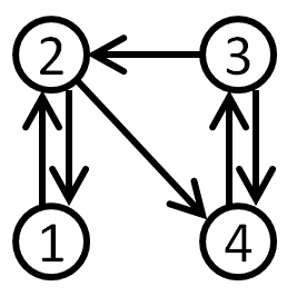
Figure 3. A graph with four vertices

Output: No identifiable scaling reparametrization exists since $d=6$ does not equal $m+1=7$.

Example 6.4.

Input: The graph $G$ in Figure 4, with the associated linear ODE system:

$$\begin{pmatrix}\dot{x}_{1}\\ \dot{x}_{2}\\ \dot{x}_{3}\\ \dot{x}_{4}\\ \dot{x}_{5}\end{pmatrix}={\begin{pmatrix}a_{11}&0&a_{13}&0&a_{15}\\ a_{21}&a_{22}&0&0&0\\ a_{31}&a_{32}&a_{33}&a_{34}&0\\ 0&0&a_{43}&a_{44}&0\\ 0&0&0&a_{54}&a_{55}\end{pmatrix}}{\begin{pmatrix}x_{1}\\ x_{2}\\ x_{3}\\ x_{4}\\ x_{5}\end{pmatrix}}+{\begin{pmatrix}u_{1}\\ 0\\ 0\\ 0\\ 0\end{pmatrix}}$$

$$y=x_{1}.$$

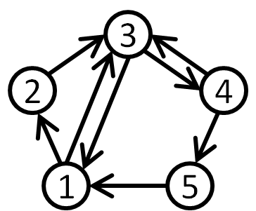
Figure 4. A graph with five vertices

Output: The following identifiable scaling reparametrization:

$$\begin{pmatrix}\dot{X}_{1}\\ \dot{X}_{2}\\ \dot{X}_{3}\\ \dot{X}_{4}\\ \dot{X}_{5}\end{pmatrix}={\begin{pmatrix}a_{11}&0&\frac{a_{13}a_{31}}{a_{43}a_{31}a_{15}a_{54}}&0&1\\ \frac{(a_{43}a_{31}a_{15}a_{54})(a_{13}a_{32}a_{21})}{a_{13}a_{31}}&a_{22}&0&0&0\\ a_{43}a_{31}a_{15}a_{54}&1&a_{33}&a_{34}a_{43}&0\\ 0&0&1&a_{44}&0\\ 0&0&0&1&a_{55}\end{pmatrix}}{\begin{pmatrix}X_{1}\\ X_{2}\\ X_{3}\\ X_{4}\\ X_{5}\end{pmatrix}}+{\begin{pmatrix}u_{1}\\ 0\\ 0\\ 0\\ 0\end{pmatrix}}$$

$$y=X_{1},$$

where $T$ corresponds to the edges $a_{32},a_{43},a_{54},a_{15}$, the rescaling is $X_{1}=x_{1},X_{2}=a_{32}a_{43}a_{54}a_{15}x_{2},X_{3}=a_{43}a_{54}a_{15}x_{3},X_{4}=a_{54}a_{15}x_{4},X_{5}=a_{15}x_{5}$, and the monomial cycles are $a_{13}a_{31}$, $a_{34}a_{43}$, $a_{43}a_{31}a_{15}a_{54}$, and $a_{13}a_{32}a_{21}$.

Thus, the new reparametrized model has $m+1$ algebraically independent parameters $b_{ij}$ and can be written as:

$$\begin{pmatrix}\dot{X}_{1}\\ \dot{X}_{2}\\ \dot{X}_{3}\\ \dot{X}_{4}\\ \dot{X}_{5}\end{pmatrix}={\begin{pmatrix}b_{11}&0&b_{13}&0&1\\ b_{21}&b_{22}&0&0&0\\ b_{31}&1&b_{33}&b_{34}&0\\ 0&0&1&b_{44}&0\\ 0&0&0&1&b_{55}\end{pmatrix}}{\begin{pmatrix}X_{1}\\ X_{2}\\ X_{3}\\ X_{4}\\ X_{5}\end{pmatrix}}+{\begin{pmatrix}u_{1}\\ 0\\ 0\\ 0\\ 0\end{pmatrix}}$$

$$y=X_{1}.$$

The graph $G$ is inductively strongly connected and has $2n-2$ edges, and thus $d$ automatically equals $m+1=9$.

We now describe results of our computations of small graphs and some of the conjectures those computations suggest. In particular, we highlight graphs which do have the expected dimension but this cannot be deduced from applying any of our constructions from Section 5. At present we lack a conjecture which would claim to give a complete characterization of all graphs which do have the expected dimension, but we provide conjectures on the structure in some extremal cases.

Below is a table displaying the results of our computations for all relevant graphs up to $n=5$ vertices. These computations were performed in Mathematica [17]. We compute the rank of the Jacobian of the double characteristic polynomial map at two randomly sampled points in parameter space to determine if the graph $G$ has the expected dimension.

Here we partition the graphs by the number $n$ of vertices and the number $m$ of edges with $n\leq m\leq 2n-2$. The columns of the table record the following information:

1. The number of strongly connected graphs with $n$ vertices and $m$ edges.

2. The number of graphs from A that have the expected dimension.

3. The number of strongly connected graphs up to symmetry permuting vertices $2,\ldots,n$.

4. For the maximal case, $m=2n-2$, the number of strongly connected graphs up to symmetry with an exchange.

5. The number of graphs from C that have the expected dimension.

6. For the maximal case, $m=2n-2$, the number of inductively strongly connected graphs up to symmetry.

$(n,m)$	A	B	C	D	E	F
(3,3)	2	2	1	NA	1	NA
(3,4)	9	7	5	4	4	4
(4,4)	6	6	1	NA	1	NA
(4,5)	84	54	15	NA	12	NA
(4,6)	316	166	55	34	30	26
(5,5)	24	24	1	NA	1	NA
(5,6)	720	576	32	NA	26	NA
(5,7)	6440	4052	281	NA	180	NA
(5,8)	26875	9565	1158	581	421	267

Remark.

From the table we see that, for the maximal case when $m=2n-2$, not every graph with an identifiable reparametrization is inductively strongly connected. Figure 5 displays the four graphs up to symmetry that have an identifiable reparametrization but are not inductively strongly connected, for $n=4$ and $m=6$.

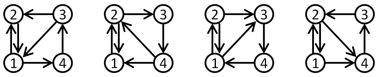
Figure 5. Graphs with an identifiable reparametrization but not inductively strongly connected

Definition 6.5.

Let $G$ be a directed graph with $n+1$ vertices labelled $0,1,2,\ldots,n$, where $0$ is the distinguished vertex corresponding to the input-output compartment. Suppose that $G$ has an exchange with vertex $1$. The collapsed graph $G^{\prime}$ is the new graph with $n$ vertices $1,\ldots,n$, where vertices $0$ and $1$ have been identified. So an edge $i\to j$ appears in $G^{\prime}$ if it appears in $G$ or if $i=1$ and $0\to j$ appears in $G$. The vertex $1$ in $G^{\prime}$ is the new distinguished vertex of the input-output compartment.

Here are two conjectures about how having the expected dimension is preserved under collapsing an exchange.

Conjecture 6.6.

Let $G$ be a graph with $n$ vertices and $2n-2$ edges with an exchange, and let $G^{\prime}$ be the resulting collapsed graph. If $G^{\prime}$ has $2n-4$ edges with an exchange, then $G$ has the expected dimension if and only if $G^{\prime}$ has the expected dimension.

Conjecture 6.7.

Let $G$ be a graph with $n$ vertices and $\leq 2n-2$ edges with an exchange, and let $G^{\prime}$ be the resulting collapsed graph. If $G^{\prime}$ has $n-1$ edges, then $G$ has the expected dimension if and only if $G^{\prime}$ has the expected dimension.

Some supporting evidence for these conjectures is provided by Proposition 5.5, where it is possible to collapse an exchange if those are the only edges incident to vertex $1$. Also, in the case where $G$ is an inductively strongly connected graph, the collapsing preserves the property of being inductively strongly connected, and hence Conjecture 6.6 is true in that case.

Proposition 6.8.

Let $G$ be an inductively strongly connected graph, and let $G^{\prime}$ be the graph obtained by collapsing the vertices in the first exchange. Then $G^{\prime}$ is inductively strongly connected.

Note that since the induced subgraph $G_{1,2}$ is strongly connected, every inductively strongly connected graph has an exchange that can be collapsed.

Proof.

We proceed by induction on the number of vertices. Let $G$ have $n$ vertices and be inductively strongly connected. Let $\tilde{G}=G_{\{1,\ldots,n-1\}}$ be the induced subgraph on the first $n-1$ vertices. This is inductively strongly connected. Its collapsing $\tilde{G}^{\prime}$ is inductively strongly connected by induction. The graph $G^{\prime}$ is obtained from $\tilde{G}^{\prime}$ by adding the vertex $n$ and at least one incoming edge to and one outgoing edge from $n$, which makes $\tilde{G}^{\prime}$ inductively strongly connected. ∎

References

- [1] S. Audoly and L. D’Angi, On the identifiability of linear compartmental systems: a revisited transfer function approach based on topological properties, Math. Biosci. 66(2) (1983) 201-228.
- [2] A. Ben-Zvi, P. J. McLellan, and K. B. McAuley, Identifiability of linear time-invariant differential-algebraic systems. 2. The differential-algebraic approach, Ind. Eng. Chem. Res. 43 (2004) 1251-1259.
- [3] N. Biggs, Algebraic Graph Theory, Cambridge University Press, Second Edition.
- [4] M. Chapman and K. Godfrey, Some extensions to the Exhaustive-Modelling Approach to structural identifiability, Math. Biosci. 77 (1985) 305-323.
- [5] M. J. Chappell and R. N. Gunn, A procedure for generating locally identifiable reparameterisations of unidentifiable non-linear systems by the similarity transformation approach, Math. Biosci. 148 (1998) 21-41.
- [6] D. Cox, J. Little, H. Schenck, Toric Varieties. Graduate Studies in Mathematics, 124. American Mathematical Society, Providence, RI, 2011.
- [7] L. Denis-Vidal and G. Joly-Blanchard, Equivalence and identifiability analysis of uncontrolled nonlinear dynamical systems, Automatica 40 (2004) 287-292.
- [8] N. D. Evans and M. J. Chappell, Extensions to a procedure for generating locally identifiable reparameterisations of unidentifiable systems, Math. Biosci. 168 (2000) 137-159.
- [9] L. Garcia-Puente, S. Spielvogel, and S. Sullivant. Identifying causal effects with computer algebra. Uncertainty in Artificial Intelligence, Proceedings of the 26th Conference, AUAI Press, 2010.
- [10] K. Godfrey and M. Chapman, Identifiability and indistinguishability of linear compartmental models, Math. and Comp. in Sim. 32 (1990) 273-295.
- [11] L. Ljung and T. Glad, On global identifiability for arbitrary model parameterization, Automatica 30(2) (1994) 265-276.
- [12] N. Meshkat, M. Eisenberg, and J. J. DiStefano III, An algorithm for finding globally identifiable parameter combinations of nonlinear ODE models using Gröbner Bases, Math. Biosci. 222 (2009) 61-72.
- [13] N. Meshkat, C. Anderson, and J. J. DiStefano III, Alternative to Ritt’s Pseudodivision for finding the input-output equations of multi-output models, Math. Biosci. 239 (2012) 117-123.
- [14] H. Miao, X. Xia, A. Perelson, H. Wu, On identifiability of nonlinear ODE models and applications in viral dynamics, SIAM Review 53 (2011), No. 1, pp. 3-39.
- [15] A. Schrijver. Theory of Linear and Integer Programming. Wiley-Interscience Series in Discrete Mathematics. A Wiley-Interscience Publication. John Wiley & Sons, Ltd., Chichester, 1986.
- [16] B. Sturmfels. Gröbner Bases and Convex Polytopes, AMS Press, Providence, 1996.
- [17] Wolfram Research, Inc., Mathematica, Version 8.0, Champaign, IL (2010).