Comparison of progenitor mass estimates for the type IIP SN 2012A
Abstract
We present the one-year long observing campaign of SN 2012A which exploded in the nearby (9.8 Mpc) irregular galaxy NGC 3239. The photometric evolution is that of a normal type IIP supernova, but the plateau is shorter and the luminosity not as constant as in other supernovae of this type. The absolute maximum magnitude, with mag, is close to the average for SN IIP. Thanks also to the strong flux in the early phase, SN 2012A reached a peak luminosity of about 2 1042 erg s-1, which is brighter than those of other SNe with a similar 56Ni mass. The latter was estimated from the luminosity in the exponential tail of the light curve and found to be M M⊙, which is intermediate between standard and faint SN IIP.
The spectral evolution of SN 2012A is also typical of SN IIP, from the early spectra dominated by a blue continuum and very broad ( 104 km s-1) Balmer lines, to the late-photospheric spectra characterized by prominent P-Cygni features of metal lines (Fe II, Sc II, Ba II, Ti II, Ca II, Na I D). The photospheric velocity is moderately low, km s-1 at 50 days, for the low optical depth metal lines. The nebular spectrum obtained 394 days after the shock breakout shows the typical features of SNe IIP and the strength of the [O I] doublet suggests a progenitor of intermediate mass, similar to SN 2004et ().
A candidate progenitor for SN 2012A has been identified in deep, pre-explosion -band Gemini North (NIRI) images, and found to be consistent with a star with a bolometric magnitude (log dex). The magnitude of the recovered progenitor in archival images points toward a moderate-mass star as the precursor of SN 2012A.
The explosion parameters and progenitor mass were also estimated by means of a hydrodynamical model, fitting the bolometric light curve, the velocity and the temperature evolution. We found a best fit for a kinetic energy of 0.48 foe, an initial radius of cm and ejecta mass of . Even including the mass for the compact remnant, this appears fully consistent with the direct measurements given above.
keywords:
supernovae: general – supernovae: individual: SN 2012A – galaxies: individual: NGC 3239 – galaxies: abundances1 Introduction
Supernovae of type IIP (SNe IIP) form a major group of core-collapse supernovae (CC SNe) characterized by a months long phase of almost constant luminosity, called the plateau. These events originate from the collapse of massive stars that, at the time of explosion, retain a massive hydrogen envelope. The ejecta, that is fully ionized by the initial shock breakout, cools down with the expansion of the SN and recombines powering the long plateau phase. A number of papers have shown that SNe IIP can be fruitfully used as distance indicators. Different methods have been applied to successfully determine extragalactic distances, including the Expanding Photosphere Method (EPM; Schmidt, Kirshner, & Eastman, 1992; Hamuy et al., 2001; Leonard et al., 2002; Dessart & Hillier, 2005; Jones et al., 2009), the Spectral-fitting Expanding Atmosphere Model (SEAM; Baron et al., 2004) and the Standardized Candle Method (Hamuy & Pinto, 2002; Nugent et al., 2006; Poznanski et al., 2009; Olivares E. et al., 2010; D’Andrea et al., 2010; Maguire et al., 2010a). The application of all of these techniques requires well monitored light curves and high-quality spectral time series. Unfortunately only a limited number of type IIP SNe fulfill the required criteria.
One well-tested approach to determine the properties of the progenitors of SNe IIP is through the modeling of the SN data with hydrodynamical codes (e.g. Grassberg, Imshennik, & Nadyozhin, 1971; Falk & Arnett, 1977; Litvinova & Nadezhin, 1983; Blinnikov et al., 2000; Utrobin, 2007; Utrobin, Chugai, & Pastorello, 2007; Utrobin & Chugai, 2008; Pumo & Zampieri, 2011; Bersten et al., 2012). The results of type IIP SN modeling have confirmed that these SNe are produced by the explosions of massive () red supergiant (RSG) stars.
An alternative approach for studing CC SNe is to search for their progenitors in deep pre-explosion images (see Smartt, 2009a, for a review). This has been done for a sample of SNe by Smartt et al. (2009b), who showed that the SNe IIP progenitor masses were confined to the range , although dust effects may increase this upper limit (Walmswell & Eldridge, 2012). On the other hand the theoretical expectation is that stars with masses up to 2530 M⊙ becames RSGs and explode as type IIP SNe. Since no star with mass above 1517 M⊙ has been seen to follow this path, there is an apparent discrepancy between theory and observations that has been termed the Red Supergiant Problem (Smartt et al., 2009b).
However, we note that there have been claims of a discrepancy between hydrodynamical and direct progenitor mass measurements for specific SNe (Smartt, 2009a) that, in view of the still large uncertainties of both approaches, leave the issue still open to discussion. Therefore any opportunities for a direct comparison between these techniques are worthy of study.
SN 2012A exploded in a very nearby host galaxy (D10 Mpc) and is a first-rate target for studying the properties of the explosion and the progenitor star. This, and the fact that SN 2012A has good pre-explosion images available in public image archives, made this object as an ideal target for an extensive follow-up campaign at multiple wavelengths. In this paper we present the results of this monitoring campaign and discuss the implication for the SN progenitor star.
The paper is organized as follows: in Section 2 we give some information about the discovery and the follow-up observations of SN 2012A, in Section 3 we present the optical and NIR photometric evolution of SN 2012A and we compare light curves, colour curves and the computed bolometric luminosity with those of other type IIP SN. In Section 4 we analyze the spectroscopic data, in Section 5 we discuss the nature of the progenitor of this SN, both by direct detection in the pre-discovery images and by modeling of the observed data. Finally, in Sections 6 and 7 we discuss and summarize the main results of the paper.
2 Discovery and follow-up observations
SN 2012A was discovered by Moore et al. (2012) in an image of the irregular galaxy NGC 3239 taken on 2012 Jan 7.39 UT. The discoverers reported that the transient was not visible on 2011 Dec 29 providing a useful constraint on the explosion epoch. Spectroscopic classification obtained on Jan 10.45 UT confirmed that the transient was a type II SN close to explosion (Stanishev & Pursimo, 2012). Indeed a comparison with a library of supernova spectra via the GELATO spectral classification tool (Harutyunyan et al., 2008) gives a best match with the type IIP SN 1999em (Elmhamdi et al., 2003a) soon after explosion.
The SN caught our interest when it turned out that deep, high spatial resolution prediscovery images were available allowing for the possible identification of the SN progenitor (Prieto et al., 2012, cf. Section 5.1). We immediately commenced an extensive campaign of photometric and spectroscopic monitoring that started three days after discovery and ended 407 days later.
The main information on the SN and host galaxy is reported in Table 1.
We note that the SN was also detected in -rays based on Swift observations obtained in the first three weeks after explosion (Pooley & Immler, 2012). As discussed in Section 3.4, it turned out that the -ray detection corresponds to a negligible contribution to the bolometric flux.
| Host galaxy | NGC 3239 |
|---|---|
| Galaxy type | IB(s)m pec |
| Heliocentric velocity | 753 3 km s-1 |
| Distance modulus | 29.96 0.15 mag |
| Galactic extinction AB | 0.117 mag |
| SN type | IIP |
| RA(J2000.0) | 10h25m07.39s |
| Dec(J2000.0) | +17∘09′146 |
| Offset from nucleus | 2465 E 161 S |
| Date of discovery | 2012 Jan 07.39 UT |
| Estimated date of explosion | MJD= |
| Mag at maximum | mag |
| at maximum | erg s-1 |
3 Photometry
Our detailed optical and infrared photometric monitoring of SN 2012A was obtained using a large number of observing facilities, listed in Table 2, where for each telescope we detail the associated instrument, the observing site, the field of view and the pixel scale.
| Telescope | Instrument | Site | FoV | Scale |
| [arcmin2] | [arcsec pix-1] | |||
| Optical facilities | ||||
| Schmidt 67/92cm | SBIG | Asiago, Mount Ekar (Italy) | 0.86 | |
| Copernico 182cm | AFOSC | Asiago, Mount Ekar (Italy) | 0.48 | |
| Prompt 41cm | PROMPT | CTIO Observatory (Chile) | 0.59 | |
| Calar Alto 2.2m | CAFOS | Calar Alto Observatory (Spain) | 0.53 | |
| NOT 2.56m | ALFOSC | Roque de los Muchachos, La Palma, Canarias (Spain) | 0.19 | |
| Trappist 60cm | TRAPPISTCAM | ESO La Silla Observatory (Chile) | 0.65 | |
| ESO NTT 3.6m | EFOSC2 | ESO La Silla Observatory (Chile) | 0.24 | |
| TNG 3.6m | LRS | Roque de los Muchachos, La Palma, Canarias (Spain) | 0.25 | |
| Infrared facilities | ||||
| REM 60cm | REMIR | ESO La Silla Observatory (Chile) | 1.22 | |
| ESO NTT 3.6m | SOFI | ESO La Silla Observatory (Chile) | 0.29 | |
| NOT 2.56m | NOTCAM | Roque de los Muchachos, La Palma, Canarias (Spain) | 0.23 | |
All frames were pre-processed using standard procedures in iraf for bias subtraction, flat fielding and astrometric calibration. For infrared exposures we also applied an illumination correction and sky background subtraction. For later epochs, multiple exposures obtained in the same night and filter were combined to improve the signal-to-noise ratio.
To measure the SN magnitude we used a dedicated pipeline developed by one of us (EC), consisting of a collection of python scripts calling standard iraf tasks (through pyraf), and specific data analysis tools such as sextractor for source extraction and classification, daophot for PSF fitting and hotpants111http://www.astro.washington.edu/users/becker/hotpants.html for PSF matching and image subtraction.
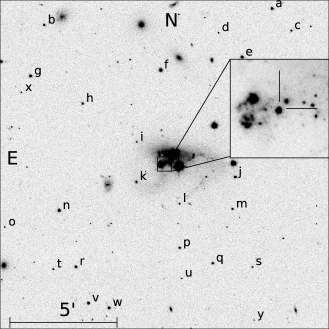
Following common practice for transient photometry, as a first step we calibrated a sequence of local standards in the field. To this aim we selected among our observations those obtained on photometric nights in which standard photometric fields from the list of Landolt (1992) were also observed. These observations were used to derive the zero point and colour term for each specific instrumental set-up and to calibrate the selected stars in the SN field (see Figure 1 and Table 3). The local sequence was used to calibrate non-photometric nights. For the infrared photometry we used as reference for the calibration 2MASS stars in the SN field.
| id | R.A. | Dec. | |||||
|---|---|---|---|---|---|---|---|
| a | 10:24:47.574 | 17:16:00.82 | 16.371 (0.027) | 16.08 (0.003) | 15.311 (0.003) | 14.878 (0.003) | 14.480 (0.004) |
| b | 10:25:29.287 | 17:15:20.22 | 16.591 (0.017) | 16.64 (0.009) | 16.261 (0.006) | 16.007 (0.010) | 15.788 (0.011) |
| c | 10:24:44.117 | 17:15:02.38 | 18.344 (0.036) | 17.89 (0.013) | 17.003 (0.014) | 16.530 (0.021) | 16.127 (0.011) |
| d | 10:24:57.404 | 17:14:58.00 | 20.420 (0.117) | 19.07 (0.046) | 17.563 (0.017) | 16.601 (0.011) | 15.152 (0.016) |
| e | 10:24:53.106 | 17:13:53.92 | 16.224 (0.027) | 15.80 (0.005) | 15.007 (0.005) | 14.562 (0.007) | 14.186 (0.009) |
| f | 10:25:08.015 | 17:13:20.67 | 14.954 (0.026) | 14.74 (0.003) | 14.043 (0.004) | 13.649 (0.004) | 13.281 (0.005) |
| g | 10:25:31.827 | 17:13:06.34 | 15.836 (0.015) | 15.82 (0.004) | 15.129 (0.003) | 14.693 (0.004) | 14.280 (0.006) |
| h | 10:25:22.336 | 17:11:54.18 | 18.156 (0.027) | 17.01 (0.005) | 15.539 (0.011) | 14.601 (0.007) | 13.496 (0.010) |
| i | 10:25:12.441 | 17:10:12.55 | 17.353 (0.029) | 17.49 (0.021) | 17.015 (0.010) | 16.731 (0.013) | 16.429 (0.016) |
| j | 10:24:54.466 | 17:08:39.59 | 16.189 (0.027) | 16.04 (0.004) | 15.346 (0.006) | 14.955 (0.016) | 14.594 (0.011) |
| k | 10:25:12.540 | 17:08:27.78 | 18.491 (0.038) | 17.15 (0.008) | 15.821 (0.005) | 14.913 (0.011) | 14.060 (0.007) |
| l | 10:25:04.672 | 17:07:30.29 | 17.990 (0.033) | 18.05 (0.015) | 17.377 (0.013) | 16.985 (0.009) | 16.550 (0.034) |
| m | 10:24:54.973 | 17:07:15.56 | 16.708 (0.028) | 16.83 (0.008) | 16.262 (0.002) | 15.932 (0.008) | 15.594 (0.011) |
| n | 10:25:26.693 | 17:07:13.71 | 16.100 (0.016) | 15.47 (0.004) | 14.454 (0.005) | 13.906 (0.003) | 13.361 (0.002) |
| o | 10:25:36.645 | 17:06:30.60 | 20.000 (0.038) | 18.99 (0.033) | 17.481 (0.017) | 16.476 (0.023) | 15.313 (0.022) |
| p | 10:25:04.685 | 17:05:34.11 | 18.309 (0.036) | 17.15 (0.005) | 15.995 (0.009) | 15.198 (0.019) | 14.533 (0.007) |
| q | 10:24:58.654 | 17:04:53.79 | 16.692 (0.028) | 16.39 (0.007) | 15.613 (0.007) | 15.156 (0.012) | 14.732 (0.005) |
| r | 10:25:23.644 | 17:04:45.78 | 16.238 (0.027) | 16.18 (0.006) | 15.530 (0.009) | 15.176 (0.006) | 14.804 (0.009) |
| s | 10:24:51.407 | 17:04:43.36 | 17.649 (0.030) | 17.80 (0.015) | 17.206 (0.015) | 16.819 (0.018) | 16.489 (0.019) |
| t | 10:25:27.785 | 17:04:39.95 | 17.282 (0.029) | 17.52 (0.015) | 16.980 (0.006) | 16.679 (0.013) | 16.357 (0.019) |
| u | 10:25:04.368 | 17:04:14.31 | 20.092 (0.093) | 18.97 (0.032) | 17.614 (0.018) | 16.681 (0.024) | 15.880 (0.013) |
| v | 10:25:21.392 | 17:03:10.35 | 17.556 (0.021) | 16.34 (0.004) | 14.953 (0.009) | 14.011 (0.008) | 13.097 (0.005) |
| w | 10:25:17.623 | 17:02:58.08 | 16.175 (0.017) | 16.00 (0.008) | 15.293 (0.007) | 14.887 (0.004) | 14.514 (0.009) |
| x | 10:25:33.513 | 17:12:23.65 | 18.403 (0.029) | 18.39 (0.017) | 17.802 (0.021) | 17.436 (0.021) | |
| y | 10:24:51.160 | 17:02:24.45 | 20.088 (0.031) | 19.16 (0.019) | 18.192 (0.014) | 17.535 (0.033) |
The region around the SN location is crowded with many sources which require special care in the measurement of the transient instrumental magnitude, in particular when the SN becomes faint and/or the seeing is poor. As a rule, the SN magnitude was measured via PSF fitting. In our implementation of the PSF fitting procedure first the sky background at the SN location is estimated by a low order polynomial fit and subtracted from the image before performing a simultaneous fit of the SN and the nearby companion stars (that is all stellar sources in a radius of FHWM from the SN) using the PSF model derived from isolated field stars. The fitted sources are removed from the original images, an improved estimate of the local background is derived and the PSF fitting procedure iterated. The residuals are visually inspected to validate the fit.
An alternative approach for the measurement of transient magnitudes is template subtraction. The application of this technique requires exposures of the field obtained before the SN explosion or after the SN has faded. The template images need to be in the same filter and have good S/N and seeing. While in principle they should be obtained with the same telescope as the specific SN observation (to guarantee the same bandpass), in practice we are bound to what is actually available in the accessible image archives. In the case of SN 2012A we could retrieve deep pre-discovery exposures in bands obtained with the Vatican Advanced Telescope Technology (VATT) and and band exposures from SDSS. For the infrared bands we rely on moderate quality 2MASS exposures.
For template subtraction, first the template image is geometrically registered to the same pixel grid as the SN frame, and thereafter the PSF of the two images is matched by means of a convolution kernel determined by comparing a number of reference sources in the field. After matching the photometric scale, the template image is subtracted from the SN image and a difference image is obtained where only the transient is present. Again, the instrumental magnitude of the transient in the difference image is measured through a PSF fit, where the model PSF is derived from the image with the worst seeing. It is found that the latter procedure is more robust with respect to plain aperture photometry in particular concerning the background level determination.
When we compare the PSF fitting vs. template subtraction measured magnitudes we find that they are in excellent agreement when the transient is bright. As a rule we kept the PSF fitting magnitudes when the discrepancy is mag and instead adopted the template subtraction magnitudes when the discrepancy is larger. For the optical bands this occurs for mag whereas for infrared the same threshold is mag .
Error estimates were obtained through artificial star experiments in which a fake star, of magnitude similar to that of the SN, is placed in the PSF fit residual image in a position close to, but not coincident with that of the real source. The simulated image is processed through the PSF fitting procedure and the dispersion of measurements out of a number of experiments, with the fake star in slightly different positions, is taken as an estimate of the instrumental magnitude error, that mainly accounts for the background fitting uncertainty. This is combined (in quadrature) with the PSF fit error returned by daophot, and the propagated errors from the photometric calibration.
The final calibrated SN magnitudes are listed in Table 4 and 7 for the optical bands and in Table 6 for the infrared.
Our light curves were complemented with -optical photometry of SN 2012A obtained using UVOT on board of the Swift satellite and recently published by Pritchard et al. (2013). This includes measurements in three filters with central wavelengths in the range Å, most useful for the derivation of the bolometric luminosity (cf. Section 3.4), as well as additional optical photometry.
| Date | MJD | Instrument | |||||
|---|---|---|---|---|---|---|---|
| 20120110 | 55936.25 | 13.16 (0.07) | 14.12 (0.02) | 14.22 (0.02) | 13.89 (0.04) | 14.23 (0.06) | ALFOSC |
| 20120110 | 55937.00 | 13.92 (0.02) | 13.94 (0.01) | 13.87 (0.02) | 13.75 (0.02) | SBIG | |
| 20120111 | 55937.25 | 14.09 (0.03) | 14.03 (0.04) | 13.84 (0.03) | 13.80 (0.02) | PROMPT | |
| 20120112 | 55938.03 | 13.94 (0.02) | 13.91 (0.02) | 13.79 (0.03) | 13.71 (0.03) | SBIG | |
| 20120112 | 55938.22 | 14.14 (0.07) | 13.99 (0.02) | 13.90 (0.04) | 13.78 (0.04) | PROMPT | |
| 20120112 | 55938.97 | 13.93 (0.04) | 13.89 (0.03) | 13.79 (0.03) | 13.71 (0.02) | SBIG | |
| 20120113 | 55939.25 | 14.06 (0.03) | 14.07 (0.05) | 13.74 (0.04) | 13.72 (0.04) | PROMPT | |
| 20120114 | 55940.03 | 13.86 (0.02) | 13.85 (0.02) | 13.66 (0.02) | 13.65 (0.02) | SBIG | |
| 20120114 | 55940.26 | 13.94 (0.03) | 14.01 (0.01) | 13.82 (0.02) | 13.73 (0.02) | PROMPT | |
| 20120114 | 55940.92 | 13.92 (0.02) | 13.84 (0.02) | 13.68 (0.03) | 13.69 (0.02) | SBIG | |
| 20120115 | 55941.97 | 13.96 (0.03) | 13.83 (0.02) | 13.71 (0.03) | 13.68 (0.02) | SBIG | |
| 20120118 | 55944.05 | 13.98 (0.04) | 13.85 (0.04) | 13.67 (0.03) | 13.64 (0.03) | SBIG | |
| 20120121 | 55947.22 | 14.20 (0.02) | 13.96 (0.01) | 13.71 (0.05) | 13.61 (0.02) | PROMPT | |
| 20120121 | 55947.93 | 13.85 (0.05) | 14.26 (0.02) | 13.97 (0.01) | 13.75 (0.03) | 13.70 (0.07) | AFOSC |
| 20120123 | 55949.96 | 14.26 (0.03) | 14.39 (0.02) | 14.01 (0.05) | 13.69 (0.03) | 13.47 (0.04) | AFOSC |
| 20120124 | 55950.93 | 14.26 (0.02) | 14.33 (0.01) | 13.91 (0.04) | 13.60 (0.02) | 13.52 (0.05) | AFOSC |
| 20120125 | 55951.21 | 14.48 (0.26) | PROMPT | ||||
| 20120125 | 55951.93 | 14.37 (0.03) | 13.87 (0.02) | 13.63 (0.04) | 13.57 (0.03) | SBIG | |
| 20120126 | 55952.23 | 14.05 (0.08) | 13.78 (0.14) | 13.61 (0.02) | PROMPT | ||
| 20120127 | 55953.05 | 14.56 (0.04) | 14.61 (0.05) | 14.06 (0.03) | 13.56 (0.03) | 13.52 (0.04) | AFOSC |
| 20120127 | 55953.88 | 14.63 (0.07) | 14.65 (0.09) | 14.11 (0.03) | 13.65 (0.05) | 13.55 (0.12) | AFOSC |
| 20120129 | 55955.94 | 15.00 (0.03) | 14.75 (0.04) | 14.11 (0.02) | 13.71 (0.02) | 13.63 (0.04) | AFOSC |
| 20120130 | 55956.93 | 15.38 (0.03) | 14.81 (0.02) | 14.13 (0.03) | 13.79 (0.04) | 13.68 (0.06) | AFOSC |
| 20120203 | 55960.93 | 14.09 (0.04) | 13.71 (0.04) | 13.67 (0.04) | SBIG | ||
| 20120208 | 55965.15 | 14.26 (0.10) | 13.86 (0.06) | SBIG | |||
| 20120208 | 55965.93 | 15.02 (0.04) | 14.15 (0.03) | 13.76 (0.07) | 13.61 (0.05) | SBIG | |
| 20120209 | 55966.19 | 15.11 (0.04) | 14.27 (0.05) | 13.82 (0.05) | 13.60 (0.04) | PROMPT | |
| 20120211 | 55968.08 | 15.63 (0.03) | 15.20 (0.05) | 14.34 (0.01) | 13.86 (0.02) | 13.62 (0.02) | CAFOS |
| 20120214 | 55971.18 | 15.19 (0.03) | 14.30 (0.03) | 13.93 (0.04) | 13.67 (0.03) | PROMPT | |
| 20120217 | 55974.17 | 15.34 (0.04) | 14.38 (0.02) | 13.89 (0.03) | 13.60 (0.03) | PROMPT | |
| 20120217 | 55974.97 | 16.44 (0.04) | 15.35 (0.02) | 14.29 (0.02) | 13.87 (0.05) | AFOSC | |
| 20120218 | 55975.97 | 16.28 (0.06) | 15.50 (0.02) | 14.43 (0.03) | 13.82 (0.04) | 13.66 (0.06) | AFOSC |
| 20120221 | 55978.31 | 14.38 (0.02) | 13.93 (0.04) | 13.66 (0.03) | PROMPT | ||
| 20120223 | 55980.04 | 16.45 (0.07) | 15.53 (0.03) | 14.42 (0.03) | 14.00 (0.04) | 13.68 (0.05) | AFOSC |
| 20120224 | 55981.20 | 15.46 (0.03) | 14.41 (0.04) | 13.96 (0.03) | 13.68 (0.03) | PROMPT | |
| 20120226 | 55983.01 | 16.66 (0.04) | 15.50 (0.02) | 14.42 (0.02) | 13.81 (0.02) | 13.80 (0.04) | AFOSC |
| 20120227 | 55984.14 | 15.53 (0.05) | 14.41 (0.02) | 13.99 (0.03) | 13.68 (0.04) | PROMPT | |
| 20120228 | 55985.96 | 16.93 (0.06) | 15.62 (0.03) | 14.50 (0.04) | 13.97 (0.02) | 13.75 (0.05) | AFOSC |
| 20120229 | 55986.14 | 15.47 (0.14) | PROMPT | ||||
| 20120301 | 55987.14 | 14.48 (0.02) | 14.03 (0.04) | 13.74 (0.03) | PROMPT | ||
| 20120304 | 55990.12 | 15.65 (0.03) | 14.49 (0.03) | 14.02 (0.03) | 13.66 (0.02) | PROMPT | |
| 20120306 | 55992.13 | 15.57 (0.17) | PROMPT | ||||
| 20120306 | 55992.89 | 14.45 (0.03) | 13.93 (0.03) | 13.76 (0.04) | SBIG | ||
| 20120312 | 55998.07 | 15.91 (0.02) | 14.72 (0.03) | 14.09 (0.02) | 13.84 (0.04) | CAFOS | |
| 20120312 | 55998.11 | 15.73 (0.05) | 14.57 (0.01) | 14.11 (0.02) | 13.78 (0.02) | PROMPT | |
| 20120313 | 55999.16 | 17.19 (0.06) | 15.72 (0.02) | 14.69 (0.04) | 14.12 (0.01) | 14.04 (0.05) | EFOSC |
| 20120313 | 55999.80 | 15.70 (0.03) | 14.60 (0.02) | 14.10 (0.03) | 13.87 (0.02) | SBIG | |
| 20120314 | 56000.10 | 15.78 (0.03) | 14.59 (0.03) | 14.10 (0.04) | 13.83 (0.02) | PROMPT | |
| 20120314 | 56000.85 | 15.65 (0.02) | 14.51 (0.02) | 14.07 (0.02) | 13.78 (0.02) | SBIG | |
| 20120315 | 56001.79 | 15.87 (0.02) | 14.58 (0.01) | 14.20 (0.03) | 13.91 (0.02) | SBIG | |
| 20120316 | 56002.05 | 15.64 (0.21) | PROMPT | ||||
| 20120316 | 56002.82 | 15.65 (0.02) | 14.52 (0.02) | 14.15 (0.02) | 13.79 (0.03) | SBIG | |
| 20120317 | 56003.04 | 14.71 (0.04) | 14.17 (0.03) | 13.95 (0.03) | PROMPT | ||
| 20120317 | 56003.96 | 17.23 (0.08) | 15.81 (0.03) | 14.55 (0.02) | 14.07 (0.04) | AFOSC | |
| 20120319 | 56005.12 | 15.83 (0.04) | 14.67 (0.03) | 14.19 (0.03) | 13.92 (0.03) | PROMPT | |
| 20120320 | 56006.88 | 15.73 (0.05) | 14.52 (0.02) | 14.16 (0.04) | 13.76 (0.04) | SBIG |
Optical photometry in Johnson-Cousins filters, with associated errors in parentheses. Date MJD Instrument 20120322 56008.11 15.92 (0.03) 14.70 (0.05) 14.19 (0.02) 13.96 (0.02) PROMPT 20120322 56008.83 15.87 (0.03) 14.66 (0.02) 14.24 (0.03) 14.04 (0.03) SBIG 20120324 56010.07 15.93 (0.04) 14.71 (0.03) 14.25 (0.03) 13.94 (0.01) PROMPT 20120326 56012.08 15.83 (0.14) PROMPT 20120326 56012.84 15.89 (0.05) 14.69 (0.01) 14.28 (0.02) 13.99 (0.03) SBIG 20120327 56013.01 14.90 (0.03) 14.35 (0.03) 14.07 (0.02) PROMPT 20120327 56013.86 15.93 (0.03) 14.71 (0.02) 14.43 (0.07) SBIG 20120328 56014.82 15.95 (0.05) 14.77 (0.04) 14.26 (0.05) 14.08 (0.04) SBIG 20120329 56015.81 15.90 (0.03) 14.82 (0.02) 14.37 (0.02) 14.10 (0.03) SBIG 20120330 56016.05 16.02 (0.03) 14.87 (0.03) 14.36 (0.03) 14.06 (0.02) PROMPT 20120331 56017.94 17.83 (0.17) AFOSC 20120331 56017.94 16.16 (0.04) 15.03 (0.03) 14.53 (0.01) 14.16 (0.05) AFOSC 20120403 56020.04 16.23 (0.05) 14.96 (0.02) 14.48 (0.03) 14.14 (0.03) PROMPT 20120409 56026.11 16.37 (0.07) 15.17 (0.03) 14.66 (0.03) 14.35 (0.01) PROMPT 20120412 56029.08 14.80 (0.23) 14.49 (0.09) PROMPT 20120412 56030.00 16.53 (0.02) 15.31 (0.01) 14.81 (0.03) 14.57 (0.02) ALFOSC 20120414 56032.00 16.69 (0.02) 15.39 (0.02) 14.99 (0.02) 14.56 (0.05) ALFOSC 20120417 56034.11 15.64 (0.03) 14.97 (0.03) 14.72 (0.02) PROMPT 20120419 56036.00 17.13 (0.05) 15.80 (0.05) 15.13 (0.03) 14.90 (0.02) PROMPT 20120421 56039.00 17.62 (0.10) 16.26 (0.05) 15.52 (0.04) 15.18 (0.03) PROMPT 20120422 56039.90 16.34 (0.03) 15.49 (0.04) 15.41 (0.11) SBIG 20120423 56040.04 17.87 (0.04) 16.40 (0.03) 15.67 (0.04) 15.26 (0.03) CAFOS 20120424 56041.96 18.32 (0.14) 16.79 (0.05) 15.95 (0.04) AFOSC 20120425 56042.86 18.28 (0.05) 16.77 (0.03) 16.09 (0.03) 15.70 (0.03) SBIG 20120426 56043.86 18.64 (0.07) 17.13 (0.04) 16.22 (0.05) 15.89 (0.04) SBIG 20120427 56044.82 18.58 (0.09) 17.23 (0.03) 16.34 (0.05) 15.90 (0.05) SBIG 20120501 56048.85 18.90 (0.07) 17.63 (0.04) 16.61 (0.04) 16.19 (0.04) CAFOS 20120515 56062.86 19.16 (0.15) 17.72 (0.02) 16.76 (0.03) 16.32 (0.06) CAFOS 20120529 56077.00 19.40 (0.11) 18.02 (0.10) 17.01 (0.10) TRAPPISTCAM 20120619 56097.99 19.48 (0.10) 18.03 (0.10) 17.15 (0.11) TRAPPISTCAM 20121020 56220.18 20.12 (0.15) 18.99 (0.13) AFOSC 20121021 56221.25 20.31 (0.15) 19.11 (0.14) 18.03 (0.03) 17.83 (0.03) LRS 20121109 56240.17 20.54 (0.27) 19.37 (0.14) 18.19 (0.09) 17.95 (0.23) AFOSC 20121122 56253.34 19.52 (0.11) 18.41 (0.12) TRAPPISTCAM 20121207 56268.13 20.60 (0.23) 19.45 (0.15) 18.65 (0.10) 18.25 (0.14) AFOSC 20121210 56271.15 19.55 (0.14) 18.63 (0.11) 18.45 (0.12) AFOSC 20121212 56273.28 18.67 (0.11) TRAPPISTCAM 20130203 56326.25 20.86 (0.15) 19.96 (0.14) 19.09 (0.14) 19.07 (0.11) LRS 20130221 56344.24 20.07 (0.09) 19.39 (0.10) TRAPPISTCAM
| Date | MJD | Instrument | |||
|---|---|---|---|---|---|
| 20120111 | 55937.23 | 14.15 (0.16) | 13.72 (0.17) | 13.55 (0.18) | REMIR |
| 20120112 | 55938.29 | 14.14 (0.15) | 13.71 (0.30) | 13.55 (0.26) | REMIR |
| 20120113 | 55939.35 | 13.61 (0.16) | 13.89 (0.17) | 13.44 (0.33) | REMIR |
| 20120124 | 55950.26 | 13.43 (0.32) | 13.38 (0.26) | 13.31 (0.39) | REMIR |
| 20120211 | 55968.12 | 13.38 (0.11) | 13.04 (0.14) | 13.35 (0.13) | REMIR |
| 20120216 | 55973.29 | 13.37 (0.46) | 13.09 (0.40) | 13.22 (0.32) | REMIR |
| 20120225 | 55982.08 | 13.28 (0.29) | 12.97 (0.23) | 12.98 (0.28) | REMIR |
| 20120305 | 55991.09 | 13.67 (0.17) | 13.66 (0.19) | 13.29 (0.39) | REMIR |
| 20120314 | 56000.08 | 13.56 (0.12) | 13.34 (0.17) | 13.30 (0.28) | SOFI |
| 20120315 | 56001.18 | 13.68 (0.25) | 13.31 (0.16) | 13.15 (0.14) | SOFI |
| 20120325 | 56011.01 | 13.83 (0.18) | 13.32 (0.06) | 13.47 (0.14) | REMIR |
| 20120405 | 56022.11 | 13.78 (0.04) | 13.70 (0.06) | 13.65 (0.20) | REMIR |
| 20120412 | 56029.11 | 14.18 (0.19) | 13.92 (0.08) | 14.11 (0.16) | REMIR |
| 20120416 | 56033.10 | 14.34 (0.23) | 14.01 (0.07) | 14.14 (0.08) | REMIR |
| 20120421 | 56038.10 | 14.66 (0.07) | 14.47 (0.10) | 14.30 (0.14) | REMIR |
| 20120507 | 56054.00 | 15.35 (0.29) | 14.93 (0.12) | 14.91 (0.16) | NOTCAM |
3.1 Photometric evolution
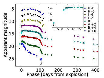
The multicolour light curves of SN 2012A are shown in Figure 2. We included the pre-discovery limit and the discovery and confirmation magnitudes from Moore et al. (2012) that, although unfiltered, are crucial to constrain the epoch of explosion. Indeed, when compared with our -band photometry, these observations appear to describe a very steep rise to maximum and indicate MJD= as the best estimate for the epoch of explosion.
In typical SNe IIP, after the fast rise, the light curve settles on a plateau phase during which the luminosity remains roughly constant, sustained by the recombination of the hydrogen envelope which was fully ionized after shock breakout. Actually, in the case of SN 2012A the luminosity in the plateau phase was never really constant: between 20 and 80 days, the magnitude decline rate is indeed small in the -band [], but already significant in the -band [] and is largest in the -band []. For comparison, in the same period SN 1999em (cf. Elmhamdi et al., 2003a) brightened in the -band at a rate of , declined by only in the -band and had a similar decline in the -band of .
We note that the behavior in the different bands of SN 2012A does not appear to be driven by a decrease of the photospheric temperature in the envelope that, as expected in the recombination phase, remains more or less constant (cf. Figure 11). Most likely the evolution in the plateau phase is related to changes in line opacities in the outer envelope regions.
At the end of hydrogen recombination the light curves of type IIP SNe show a sudden drop in luminosity. In the case of SN 2012A this occurs about 90 days after explosion, days earlier than for SN 1999em. The period of rapid luminosity decline terminates at about days after a drop in the -band of 2 mag. After this, the light curves settle onto a much shallower linear decline powered by the radioactive decay of 56Co into 56Fe. Indeed, the decline rate in and bands measured in the phase range is , very close to the expected energy input from 56Co decay, .
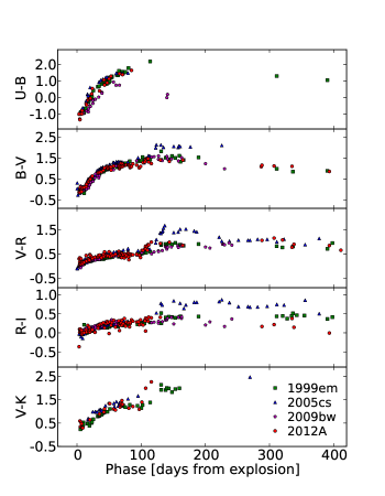
The , , , and colour curves of SN 2012A are shown in Figure 3 and compared to those of SNe 1999em (Elmhamdi et al., 2003a), 2009bw (Inserra et al., 2012) and 2005cs (Pastorello et al., 2006; Pastorello et al., 2009). The choice of these SNe as references is justified by the fact that, as will be shown in the following, they appear to bracket SN 2012A in a number of properties, including luminosity, expansion velocity, temperature and 56Ni-mass.
The colours of SN 2012A have been corrected for the sum of the adopted Galactic and host galaxy extinction, that is mag (cf. Section 4.4), whereas for the comparison SNe we adopted the extinction corrections given in the quoted papers. In all colours the evolution of the four SNe is remarkably similar up to 100 days from explosion. The rapid colour evolution seen in the first month (especially in the colour) is a result of the expansion and cooling of the SN photosphere. After days, the colours of SN 2012A show very little evolution, similar to the behaviour of SNe 1999em and 2009bw, whereas SN 2005cs shows a sudden jump to somewhat redder colours that is a characteristic feature of many faint type II SNe (Pastorello et al., 2009).
3.2 The ugriz photometry
An increasing number of observing facilities are equipped with ugriz filters which mimic the photometric system of the Sloan Digital Sky Survey222http://www.sdss.org. Therefore one is often faced with the problem of comparing SDSS-like photometry for a SN with the template light curves available in the conventional UBVRI Johnson-Cousins system. Transformation equations have been provided by a number of authors, derived from comparisons of the magnitudes of standard stars in the two photometric systems (Chonis & Gaskell, 2008, and reference therein). However SN spectra are very different from those of typical stars, with strong absorptions and emissions, and so the validity of these transformation equations is not guaranteed.
For SN 2012A, in many respects a typical type IIP SN, we have the opportunity of direct testing the validity of these transformation equations, thanks to simultaneous observations in both systems obtained with the PROMPT telescopes at CTIO.
The griz photometry of SN 2012A, reduced with the same recipes as for the Johnson-Cousins photometry, is reported in Table 7. The photometric calibration was obtained by comparison with the SDSS magnitudes for the stars in the field of the SN and are therefore close to the AB system ( mag), whereas the Johnson-Cousins photometry reported in Table 4 are in the VEGA system.
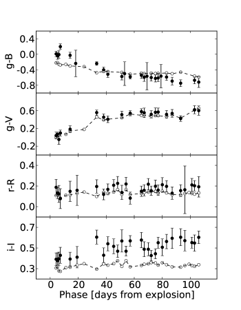
In Figure 4 we show the difference in SN magnitude in the SDSS and Johnson-Cousins systems for selected filter combinations as a function of the light curve phase. The difference between the observed magnitudes (filled circles) is compared with the expected difference (empty circles) as derived from the transformation equations of Chonis & Gaskell (2008) using the observed and colours.
Besides the systematic offset, Figure 4 shows in all bands apart from a clear trend with phase. This is largely expected because of the rapid SN colour evolution and dependence of the transformation equation on the colour. Indeed it appears that the transformation equations are a fairly good approximation for the and differences, but less valid for the and differences. While the differences in are readily attributed to the very different passbands of the two filters resulting in a different sampling of the evolving spectral energy distribution of the SN, the large systematic offset in required further analysis. It transpired that the filter of PROMPT has a somewhat redder cutoff than the SDSS filter and hence it includes the strong Ca II feature at Å that is outside of the SDSS band. This effect accounts for the offset of mag of the observed differences and those expected from the transformation equations.
We conclude that provided filters are carefully matched, transformation equations can be safely used for SNe IIP, apart from for .
| Date | MJD | Instrument | ||||
|---|---|---|---|---|---|---|
| 20120113 | 55939.25 | 14.04 ( 0.10) | 13.88 ( 0.07) | 14.12 ( 0.05) | 14.30 ( 0.05) | PROMPT |
| 20120114 | 55940.27 | 14.13 ( 0.07) | 13.90 ( 0.10) | 14.17 ( 0.07) | 14.23 ( 0.05) | PROMPT |
| 20120118 | 55944.21 | 14.07 ( 0.07) | 13.90 ( 0.04) | 14.06 ( 0.04) | 14.25 ( 0.10) | PROMPT |
| 20120121 | 55947.23 | 14.16 ( 0.08) | 13.86 ( 0.08) | 14.01 ( 0.06) | 14.15 ( 0.08) | PROMPT |
| 20120125 | 55951.22 | 14.23 ( 0.22) | PROMPT | |||
| 20120126 | 55952.24 | 13.95 ( 0.05) | 14.03 ( 0.10) | 14.16 ( 0.10) | PROMPT | |
| 20120131 | 55957.21 | 14.45 ( 0.07) | 14.09 ( 0.06) | 14.13 ( 0.08) | 14.01 ( 0.07) | PROMPT |
| 20120209 | 55966.20 | 14.86 ( 0.03) | 14.02 ( 0.04) | 14.22 ( 0.06) | 14.01 ( 0.06) | PROMPT |
| 20120214 | 55971.18 | 14.78 ( 0.06) | 14.06 ( 0.03) | 14.11 ( 0.07) | 14.14 ( 0.09) | PROMPT |
| 20120217 | 55974.18 | 14.82 ( 0.07) | 14.07 ( 0.04) | 14.15 ( 0.06) | 14.03 ( 0.04) | PROMPT |
| 20120221 | 55978.32 | 14.14 ( 0.04) | 14.18 ( 0.07) | 14.14 ( 0.07) | PROMPT | |
| 20120224 | 55981.17 | 14.20 ( 0.06) | 14.15 ( 0.06) | 14.13 ( 0.07) | PROMPT | |
| 20120227 | 55984.15 | 14.95 ( 0.07) | 14.14 ( 0.06) | 14.26 ( 0.10) | 13.99 ( 0.08) | PROMPT |
| 20120229 | 55986.14 | 14.96 ( 0.27) | PROMPT | |||
| 20120301 | 55987.14 | 14.26 ( 0.05) | 14.21 ( 0.04) | 14.19 ( 0.06) | PROMPT | |
| 20120304 | 55990.13 | 15.06 ( 0.05) | 14.11 ( 0.05) | 14.24 ( 0.05) | 14.05 ( 0.06) | PROMPT |
| 20120312 | 55998.12 | 15.17 ( 0.06) | 14.27 ( 0.04) | 14.36 ( 0.07) | 14.12 ( 0.06) | PROMPT |
| 20120314 | 56000.11 | 15.17 ( 0.10) | 14.27 ( 0.04) | 14.32 ( 0.07) | 14.13 ( 0.06) | PROMPT |
| 20120316 | 56002.07 | 15.06 ( 0.28) | PROMPT | |||
| 20120317 | 56003.05 | 14.40 ( 0.05) | 14.44 ( 0.06) | 14.24 ( 0.11) | PROMPT | |
| 20120319 | 56005.12 | 15.22 ( 0.08) | 14.35 ( 0.03) | 14.36 ( 0.04) | 14.25 ( 0.05) | PROMPT |
| 20120322 | 56008.12 | 15.29 ( 0.09) | 14.39 ( 0.06) | 14.41 ( 0.04) | 14.30 ( 0.05) | PROMPT |
| 20120324 | 56010.08 | 15.30 ( 0.09) | 14.42 ( 0.04) | 14.50 ( 0.05) | 14.34 ( 0.10) | PROMPT |
| 20120326 | 56012.10 | 15.26 ( 0.27) | PROMPT | |||
| 20120327 | 56013.04 | 14.57 ( 0.06) | 14.58 ( 0.08) | 14.48 ( 0.07) | PROMPT | |
| 20120330 | 56016.07 | 15.42 ( 0.08) | 14.56 ( 0.05) | 14.63 ( 0.07) | 14.51 ( 0.06) | PROMPT |
| 20120403 | 56020.06 | 15.53 ( 0.09) | 14.61 ( 0.05) | 14.74 ( 0.10) | 14.53 ( 0.09) | PROMPT |
| 20120409 | 56026.13 | 15.61 ( 0.06) | 14.82 ( 0.05) | 14.96 ( 0.08) | 14.64 ( 0.13) | PROMPT |
| 20120412 | 56029.11 | 14.97 ( 0.04) | 15.07 ( 0.04) | 14.79 ( 0.11) | PROMPT | |
| 20120415 | 56032.13 | 15.10 ( 0.07) | 15.16 ( 0.07) | 14.94 ( 0.09) | PROMPT | |
| 20120417 | 56034.15 | 15.19 ( 0.06) | 15.28 ( 0.05) | 15.05 ( 0.10) | PROMPT | |
| 20120419 | 56036.04 | 16.45 ( 0.07) | 15.34 ( 0.04) | 15.46 ( 0.08) | 15.21 ( 0.08) | PROMPT |
| 20120422 | 56039.04 | 16.89 ( 0.09) | 15.72 ( 0.09) | 15.79 ( 0.05) | 15.42 ( 0.22) | PROMPT |
3.3 Distance and absolute magnitudes
The Nearby Galaxies Catalog by Tully (1988) reports for NGC 3239 a distance of 8.1 Mpc, based on the measured redshift and using a model for the local velocity field. Indeed, as is well known, the redshift of nearby galaxies is perturbed by the influence of the Virgo cluster, the Great Attractor (GA), and the Shapley supercluster. It turns out that updated models of the local velocity field yield a distance that is about 20% larger than the above value, that is Mpc as also reported by the NASA/IPAC Extragalactic database (NED)333http://ned.ipac.caltech.edu. This is fully consistent with the value of Mpc reported in the Extragalactic Distance Database (Tully et al., 2009) and obtained with the same method. In the following we adopt a distance of 9.8 Mpc, i.e. a distance modulus of 29.96 mag with a formal error of 0.15 mag as reported by NED ( km s-1 Mpc-1). We also derive the total extinction in the direction of NGC 3239 (Galactic plus host galaxy) as mag (see Section 4.4).
The SN apparent magnitudes at maximum were estimated through a low order polynomial fit of the early light curves ( 30 d), from which we obtained mag, mag and mag, where the error budget is dominated by the fact that, with the exception of the -band, the rise to the maximum light is not really well constrained. Keeping in mind this uncertainty in the detection of maximum epoch, we derived SN absolute magnitudes at maximum of mag, mag, mag, close to the average for SNe IIP (Li et al., 2011). In particular at maximum SN 2012A was very similar to SN 1999em which had mag (with a relatively large uncertainty in the host galaxy distance) and about 1 mag brighter than the faint type IIP SN 2005cs with mag.
We can use the Nugent et al. (2006) correlation between the absolute brightness of SNe IIP and the expansion velocities derived from the minimum of the Fe II 5169 Å P-Cygni feature observed during the plateau phase. Incorporating our colour and the velocity measured from the Fe II 5169 Å line at +50 d in equation (1) of Nugent et al. (2006), we find a distance modulus of mag which, within the uncertainties, is consistent with the assumed value.
3.4 Bolometric light curve
By integrating the multicolour photometry of SN 2012A from the to the near , we can derive the bolometric luminosity. In practice, for each epoch and filter, we derived the flux at the effective wavelength. When no observation in a given filter/epoch was available, the missing measurement was obtained through interpolation of the light curve in the given filter or, if necessary, by extrapolating the missing photometry assuming a constant colour from the closest available epoch. The fluxes, corrected for extinction, provide the spectral energy distribution at each epoch, which is integrated by the trapezoidal rule, assuming zero flux at the integration boundaries. The observed flux is converted into luminosity for the adopted distance.
We note that, shortly after discovery, the SN was not detected in radio setting a fairly restrictive upper limit to the radio luminosity (Stockdale et al., 2012) and that the -ray detection, even neglecting the probable contamination by nearby sources, corresponds to a negligible contribution to the bolometric flux of about (Pooley:2012a), that is of the bolometric flux in the first month after explosion.
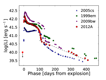
The bolometric light curve is presented in Figure 5 together with those of SNe 1999em, 2005cs and 2009bw computed with the same prescription. SN 1999em was selected as reference because it provided the best match with the early spectrum of SN 2012A as given by the automatic classification tool (cf. Section 2), while SNe 2005cs and 2009bw were chosen because they appear to encompass the observed properties of SN 2012A being fainter and brighter than SN 2012A, respectively. In fact it appears that the early luminosity of SN 2012A well matches that of SN 1999em.
We emphasize that at very early phases the far spectral range contributes almost 50% of the total bolometric luminosity, but in two weeks it drops to less than 10%. This should be taken into account when comparing with other SNe without far coverage.
As noted before, in SN 2012A the plateau luminosity is not really constant showing a monotonic decline up to days from explosion. The drop, marking the end of the hydrogen envelope recombination, begins days earlier than in most type IIP SNe, including SNe 1999em and 2005cs, and the late linear tail sets in earlier. Also we note that in SN 2012A the drop in luminosity from the plateau to the light curve tail is deeper than in SNe 1999em or 2005cs and similar to SN 2009bw. Moreover the luminosity of the linear late tail is intermediate between those of SNe 1999em and 2005cs, resembling SN 2009bw. As mentioned previously, in typical type II SNe the linear tail is powered by the energy input from 56Co decay. This is confirmed by the observed luminosity decline rate of SN 2012A that, as seen in Figure 5, matches fairly well the predicted decline assuming that all the high energy photons and positrons from the radioactive decay are fully trapped and converted into -optical radiation. In this case, the tail luminosity is a direct indicator of the amount of 56Ni (the parent element in the radioactive chain) produced in the explosion. We can therefore conclude that the 56Ni mass of SN 2012A was about half that of SN 1999em and about twice that of SN 2005cs.
For a more accurate determination of the 56Ni mass it is convenient to refer to SN 1987A for which the mass of radioactive nichel has been accurately estimated to be Ni) = 0.075 (Danziger, 1988; Woosley, Hartmann, & Pinto, 1989). The comparison of the bolometric light curves of SNe 2012A and 1987A, computed integrating the luminosity in the same spectral range, shows that from which we derive Ni) = 0.011 for SN 2012A, where the error budget is dominated by the uncertainty on the distance.
As an independent check, following Elmhamdi, Chugai, & Danziger (2003b), we estimated the steepness function , defined as steepness of the light curve at the inflection point during the rapid drop from the plateau to the radioactive tail. It was shown that is strongly correlated to the ejected 56Ni mass (cf. Figure 5 in Elmhamdi, Chugai, & Danziger, 2003b). From a value of mag d-1 for SN 2012A, we calculate Ni) = 0.015, which is in good agreement with the value derived from the observed luminosity in the radioactive tail.
The ejected mass of 56Ni derived for SN 2012A is intermediate between those of prototypical SNe IIP, e.g. SNe 1969L and 1988A for which Ni) = 0.07 (Turatto et al., 1993), and the value for underluminous SNe IIP (Pastorello et al., 2004), e.g. SNe 1997D and 2005cs, for which Ni) = 0.002 and 0.003 , respectively (Turatto et al., 1998; Benetti et al., 2001; Pastorello et al., 2009). A similar 56Ni mass was found for SN 2009bw [Ni) = 0.022 , cf. Inserra et al. (2012)].
4 Spectroscopy
Spectroscopic observations of SN 2012A were carried out with several telescopes commencing short after explosion, continued for well over one year, and yielding a total of 47 epochs of medium/low resolution spectroscopy. In addition, high-resolution spectra were obtained at four epochs. The journal of the spectroscopic observations is given in Table 8. For each spectrum we report: the date, MJD and phase from explosion, the telescope and the instrumental configuration, the spectral range and, finally, the resolution, estimated from the FWHM of the night sky lines.
Data reduction was performed using standard iraf tasks. Spectral images were bias and flat-field corrected, before the SN spectrum was extracted by tracing the stellar profile along the spectral direction and subtracting the sky background along the slit direction. Wavelength calibration was accomplished by obtaining comparison lamp spectra, while for flux calibration we referred to the observations of spectrophotometric standard stars obtained, when possible, in the same nights as the SN. The flux calibration of all spectra was verified against photometry and corrected, if necessary. The telluric absorption corrections were estimated from the spectra of spectrophotometric standards. Notwithstanding this, often imperfect removal can affect the profile of the SN features that overlap with the strongest atmospheric absorptions, in particular the telluric band at Å.
For the high-resolution spectra we performed an additional check on the accuracy of the wavelength calibration by measuring the wavelength of night-sky lines (O I, OH, Hg I and Na I D, Osterbrock et al., 2000). With this we achieved an accuracy of the velocity scale of .
| Date | MJD | Phase | Instrumental | Range | Resolution |
|---|---|---|---|---|---|
| [d] | configuration1 | [Å] | [Å] | ||
| 20120109 | 55936.14 | 3.1 | NOT+ALFOSC+gm4 | 3400-9000 | 14 |
| 20120110 | 55936.95 | 3.9 | Ekar+Echelle+gr300 | 3780-7400 | 0.34 |
| 20120115 | 55941.08 | 8.1 | Ekar+Echelle+gr300 | 4060-7785 | 0.38 |
| 20120115 | 55941.21 | 8.2 | INT+IDS+R150V | 3500-10000 | 13 |
| 20120116 | 55942.14 | 9.1 | Ekar+Echelle+gr300 | 4060-7785 | 0.38 |
| 20120117 | 55943.14 | 10.1 | INT+IDS+R150V | 3500-10000 | 13 |
| 20120117 | 55943.97 | 11.0 | OHP+1.93m+Carelec | 3700-7300 | 7 |
| 20120118 | 55944.03 | 11.0 | Ekar+AFOSC+gm4,gm2 | 3500-9200 | 24 |
| 20120118 | 55944.14 | 11.1 | INT+IDS+R150V | 3500-10000 | 13 |
| 20120118 | 55944.98 | 12.0 | OHP+1.93m+Carelec | 3700-7300 | 7 |
| 20120119 | 55945.19 | 12.2 | INT+IDS+R150V | 3500-10000 | 13 |
| 20120120 | 55946.06 | 13.1 | OHP+1.93m+Carelec | 3700-7300 | 7 |
| 20120121 | 55947.00 | 14.0 | OHP+1.93m+Carelec | 3700-7300 | 7 |
| 20120121 | 55947.98 | 15.0 | Ekar+AFOSC+gm4 | 3500-8200 | 24 |
| 20120123 | 55949.98 | 17.0 | Ekar+AFOSC+gm4 | 3500-8200 | 24 |
| 20120124 | 55950.97 | 18.0 | Ekar+AFOSC+gm4 | 3500-8200 | 24 |
| 20120126 | 55952.15 | 19.1 | Pennar+B&C+300tr/mm | 3400-7800 | 10 |
| 20120127 | 55953.03 | 20.0 | Ekar+AFOSC+gm4 | 3500-8200 | 24 |
| 20120129 | 55955.97 | 22.9 | Ekar+AFOSC+gm4 | 3500-8200 | 24 |
| 20120130 | 55956.92 | 23.9 | Ekar+AFOSC+gm4 | 3500-8200 | 24 |
| 20120205 | 55962.94 | 29.9 | Pennar+B&C+300tr/mm | 3400-7800 | 10 |
| 20120210 | 55968.11 | 35.1 | CAHA+CAFOS+b200+r200 | 3400-10500 | 10 |
| 20120213 | 55970.94 | 37.9 | Pennar+B&C+300tr/mm | 3400-7800 | 10 |
| 20120218 | 55975.94 | 42.9 | Ekar+AFOSC+gm4 | 3500-8200 | 24 |
| 20120222 | 55980.00 | 47.0 | Ekar+AFOSC+gm4 | 3500-8200 | 24 |
| 20120225 | 55982.99 | 50.0 | Ekar+AFOSC+gm4 | 3500-8200 | 24 |
| 20120228 | 55985.92 | 52.9 | Ekar+AFOSC+gm4 | 3500-8200 | 24 |
| 20120306 | 55992.88 | 59.9 | Pennar+B&C+300tr/mm | 3400-7800 | 10 |
| 20120309 | 55996.43 | 63.4 | Ekar+Echelle+gr300 | 3780-7400 | 0.34 |
| 20120311 | 55998.09 | 65.1 | CAHA+CAFOS+b200 | 3300-8850 | 13 |
| 20120313 | 55999.18 | 66.2 | NTT+EFOSC2+gr11+gr16 | 3350-10000 | 12 |
| 20120315 | 56000.11 | 67.1 | NTT+SOFI+GB+GR | 9400-25000 | 20 |
| 20120315 | 56001.88 | 68.9 | Pennar+B&C+300tr/mm | 3400-7800 | 10 |
| 20120317 | 56003.91 | 70.9 | Ekar+AFOSC+gm4 | 3500-8200 | 24 |
| 20120325 | 56012.01 | 79.0 | Pennar+B&C+300tr/mm | 3400-7800 | 10 |
| 20120327 | 56013.84 | 80.8 | Ekar+AFOSC+gm4 | 3500-8200 | 24 |
| 20120329 | 56015.83 | 82.8 | Pennar+B&C+300tr/mm | 3400-7800 | 10 |
| 20120331 | 56017.90 | 84.9 | Ekar+AFOSC+gm4 | 3500-8200 | 24 |
| 20120412 | 56029.82 | 96.8 | Pennar+B&C+300tr/mm | 3400-7800 | 10 |
| 20120422 | 56040.06 | 107.1 | CAHA+CAFOS+g200 | 4100-10200 | 13 |
| 20120424 | 56041.91 | 108.9 | Ekar+AFOSC+gm4 | 3500-8200 | 24 |
| 20120427 | 56044.94 | 111.9 | Ekar+AFOSC+gm4 | 3500-8200 | 24 |
| 20120501 | 56048.89 | 115.9 | CAHA+CAFOS+g200 | 3800-10200 | 13 |
| 20120515 | 56062.87 | 129.9 | CAHA+CAFOS+g200 | 3800-10200 | 13 |
| 20120515 | 56062.89 | 129.9 | INT+IDS+R150V | 4000-9500 | 10 |
| 20120608 | 56086.89 | 153.9 | NOT+ALFOSC+gm4 | 3400-9000 | 14 |
| 20120627 | 56105.89 | 172.9 | WHT+ISIS+R300B+R158R | 3500-10000 | 5 |
| 20130203 | 56326.05 | 393.1 | TNG+LRS+LR-B,LR-R | 3350-10370 | 10 |
1 NOT = 2.56m Nordic Optical Telescope (La Palma, Spain); Ekar = Copernico 1.82m Telescope (Mt. Ekar, Asiago, Italy); INT = 2.5m Isaac Newton Telescope (La Palma, Spain); OHP = Observatoire de Haute-Provence 1.93m Telescope (France); Pennar = Galileo 1.22m Telescope (Pennar, Asiago, Italy); CAHA = Calar Alto Observatory 2.2m Telescope (Andalucia, Spain); NTT = 3.6m ESO NTT (La Silla, Chile); WHT = 4.2m William Herschel Telescope (La Palma, Spain); TNG = 3.6m Telescopio Nazionale Galileo (La Palma, Spain).
4.1 Spectral evolution


The overall spectral evolution of SN 2012A is shown in Figures 6 and 7. The first set of spectra (Figure 6) illustrates the spectral evolution during the hydrogen envelope recombination from shortly after shock breakout ( d) to the beginning of the transition phase, while the second set (Figure 7) shows the transition from the photospheric to the nebular phase.
The earlier spectra are characterized by a very blue continuum, with blackbody temperatures above K. The only prominent features are the hydrogen Balmer lines with broad P-Cygni profiles, and He I 5876 Å. After a couple of weeks, the He I 5876 Å disappears while the metal lines increase in strength, and after one month, become the dominant features (apart from H and H). The identified lines include Fe II (4500 Å, 4924, 5018 and 5169 Å), Sc II (4670 Å, 5031 Å), Ba II (6142 Å), Ca II (8498, 8542 and 8662 Å, H&K), Ti II (blended with Ca II H&K). Strong line blanketing, especially by Fe II transitions, characterizes the blue spectral region below 3800 Å, suppressing much of the flux. The Na I D feature emerges where earlier on He I 5876 Å was detected.
In the spectra between +10 to +25 d, a faint absorption feature is visible at about 6270 Å, just to the blue side of the H P-Cygni absorption. A similar feature was detected by Pastorello et al. (2006) in SN 2005cs and attributed either to high-velocity detached hydrogen (for SN 2012A km s-1) or to the Si II Å doublet. The lack of a similar absorption feature in the blue side of H (left and middle panels of Figure 8) supports the Si II identification. In this case, adopting for the Si II doublet an effective wavelength of 6355 Å, the expansion velocity as measured by fitting the P-Cygni absorption profile would be 4400 km s-1 around +12 d, and decreases to 4000 km s-1 in the following epochs. These expansion velocities are comparable to those derived from Fe II 5169 Å at similar phases (cf. Figure 12).
The evolution of H from +109 to +173 d is shown in the right panel of Figure 8. While within 100 days from explosion H was characterized by a symmetric P-Cygni profile, by day a double peaked emission starts to develop and becomes more evident in the subsequent spectra at phases d. A complex profile is seen in H as well, even though the blend of several lines prevents the recognition of multiple components there. H asymmetry was observed before in SN 1987A (Phillips & Williams, 1991; Chugai, 1991), SN 1999em (Elmhamdi et al., 2003a) and SN 2004dj (Chugai et al., 2005). For the first two SNe an asymmetric, redshifted H line was reported, while SN 2004dj showed a double peaked structure. A similar H profile clearly arises in SN 2012A by day +112, with a dominant blue peak shifted by 1000 km s-1 and a red one shifted by 1300 km s-1. As suggested by Chugai et al. (2005) and Chugai (2006) for SN 2004dj, this may indicate an asymmetric (bipolar) ejection of 56Ni in the otherwise spherically-symmetric envelope. Moreover, as for SN 2004dj, the prominence of the blue peak over the red one can be explained with a 56Ni distribution that is skewed towards the observer. In the following spectra of SN 2012A, the H profile shows some evolution, with the blue peak receding to 500 km s-1 and the red peak increasing to 1800 km s-1. Finally, in the late nebular spectrum (+394 d, see Figure 7), H shows a single narrow Gaussian profile. We note that the [Ca II] 7391, 7324 Å features seem to show a similar structure, although we cannot test with the [O I] doublet (6300, 6364 Å) as this line becomes prominent only in our last spectrum at phase +394 d.

In Figure 9 we compare the spectra of SN 2012A at about maximum, one month and one year after explosion with those of SN 1999em (Elmhamdi et al., 2003a) and SN 2005cs (Pastorello et al., 2006) taken at comparable phases. Several similarities with these SNe IIP, and in particular with SN 1999em, have already been remarked upon. All CC SNe are characterized by blue continua at the early phases with blackbody temperatures that become very similar after about one month. These three SNe also show similar spectral features, with Balmer lines and He I 5876 Å early on, and one month later the emergence of metal lines, in particular Fe II , Sc II, Ba II and the Ca II infrared triplet.

During the transition from the plateau to the radioactive tail (Figure 7), the continuum emission remains strong. This can be seen from the deep absorption of Na I and a new strong feature of O I at 7774 Å. At the same time nebular emission lines begin to emerge, first of all [Ca II] Å and subsequently [O I] Å and [Fe II] Å. The last spectrum taken at +394 d is well in the nebular phase. Along with the always strong H line, with FWHM , the most prominent lines are permitted emissions from H, Na I D and the Ca II infrared triplet and forbidden lines of [Ca II], [O I], [Fe II] and Mg I] 4572 Å. Additional emission in the range Å and around 7710 Å is most likely due to [Fe I] and [Fe II] multiplets. We also notice that bluewards of 4500 Å, the spectrum shows the signature of a blue continuum that most likely is due to contamination from a nearby hot star or association.
In Table 9 we report the measurements of the flux of the most prominent lines detected in the latest spectrum. Nebular line fluxes for a sample of SNe IIP have been collected by Maguire et al. (2012) showing only a moderate variation from object to object. Actually, for SN 2012A the Ca II and O I emission relative to H are among the weakest of the sample for the given phase, whereas the Fe II/H emission ratio is close to the average. The ratio of the two lines in the [O I] 6300, 6364 doublet is , similar to SN 2004et and close to the expected value for the thin regime, whereas for most SNe II at this phase the ratio is much lower signaling that the ejecta still has some optical depth.
Jerkstrand et al. (2012) have used their spectral synthesis code to model the nebular emission line fluxes for SN explosions of different mass progenitors, and find [O I], Na I D and Mg I] to be the most sensitive lines. By comparing their models with late time observations of the type IIP SN 2004et, they found a best match with a 15 M⊙ progenitor model. From Table 9 we derive the fractions of the line luminosities normalized to the luminosity from the 56Co decay at +394 days (assuming Ni) = 0.011 and a distance of 9.8 Mpc, cf. Sections 3.3, 3.4), finding values of 2.6% for [O I] Å, 0.70% for Na I D and 0.63% for Mg I] 4571 Å. The comparison with the expected line flux from models (see Figure 8 in Jerkstrand et al., 2012) shows that the [O I] and Na I D values are close to the 15 M⊙ track, while the Mg I] line is closest to the 19 M⊙ track. As discussed by Jerkstrand et al. (2012), the [O I] lines are more reliable mass indicators than the other ones. Therefore we conclude that the best match from the nebular spectrum analysis is for a 15 M⊙ progenitor. However, we note that the nebular models in Jerkstrand et al. (2012) are computed for a higher mass of ejected 56Ni (Ni) = 0.062 M⊙ as derived for SN 2004et). A lower 56Ni mass will result in lower ionization and temperature, somewhat altering the fraction of cooling done by various emission lines.
Maguire et al. (2012) have also shown the existence of a correlation between Ni mass and ejecta expansion velocity, measured from the FWHM of the H line. By using this relation for SN 2012A we derive Ni) = 0.022 M⊙ which, within the uncertainties is consistent with our measurement based on the late luminosity.
| Line | Flux [] |
|---|---|
| H | 4.10 |
| O I 6300 Å | 0.81 |
| O I 6363 Å | 0.31 |
| Fe II | 0.27 |
| Ca II | 1.90 |
| Na ID | 0.30 |
| Mg II | 0.27 |
| Ca II NIR | 1.00 |
4.2 Near-infrared spectrum
A near infrared (NIR) spectrum of SN 2012A was collected with NTT+SOFI during the photospheric phase (+67 days), covering the wavelength region between 9400 to 25000 Å. It is shown in Figure 10 after merging with the +66 days optical spectrum taken with the same telescope but equipped with EFOSC2. This was compared with the NIR SN spectra presented in Gerardy et al. (2001); Fassia et al. (2001); Pozzo et al. (2006) which were also used as guide for line identification. The NIR spectrum is dominated by the Paschen series of hydrogen, showing P-Cygni profiles similar to the Balmer lines. Br is also detected. In the insert of Figure 10 we show a zoomed-in-view of the NIR region between 9000 and 13000 Å. The spectral lines are typical of SNe IIP at this phase, in particular the blend of C I 10691 Å with He I 10830 Å that was also observed in coeval epochs are available, i.e. SN 1997D (Benetti et al., 2001), SN 1999em (Hamuy et al., 2001), SN 2005cs (Pastorello et al., 2009) and SN 2004et (Maguire et al., 2010b). Sr II 10327 Å is clearly visible, while the contribution of Fe II 10547 Å is not as evident as in other type II SNe (see for example SN 2005cs in Pastorello et al., 2009).

4.3 Blackbody temperature and expansion velocities
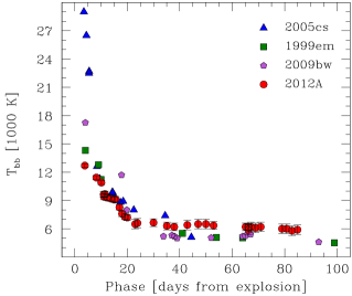
Estimates of the photospheric temperatures of SN 2012A were derived from blackbody functions fitted to the spectral continuum (the spectra were corrected for the redshift and adopted extinction), from a few days after explosion up to 80 days. Later on, due to both emerging emission lines and increased line blanketing which causes a flux deficit at the shorter wavelengths, the fitting of the continuum becomes difficult. The data are collected in Table 10, and the temperature evolution is shown in Figure 11, along with the same measurements for SNe 2005cs, 2009bw and 1999em for comparison. The errors were estimated from the dispersion of measurements obtained with different choices for the spectral fitting regions. The early photospheric temperature of SN 2012A is above 1.2 104 K, but it decreases quickly to K within three weeks and then remains roughly constant. The evolution of SN 2012A is very similar to that of SNe 1999em and 2009bw, whereas SN 2005cs showed a much higher temperature at very early phases (2.9 104 K, Pastorello et al., 2006).
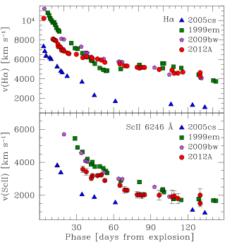
The expansion velocity of the ejecta is measured by fitting the P-Cygni absorption components of different lines, in particular H, H, Fe II 5169 Å, Sc II 5527, 6245 Å, Ba II 6142 Å and He I 5876 Å. The latter is detected in the spectra during the first two weeks after core-collapse, while after about one month, Na I D emerges in the same spectral region. The expansion velocity evolution of the different lines is shown Figure 12. H displays systematically higher velocities than other lines, which is a consequence of the high optical depth of this transition. The comparison of the H expansion velocity with that of other SNe II in Figure 13 shows once more that SN 2012A is more similar to SNe 1999em and 2009bw, whereas SN 2005cs has a much smaller velocity.
If we take the velocity of the Sc II 6245 Å line with its low optical depth as representative of the photospheric expansion velocity, we find that SN 2012A has an intermediate velocity between SNe 1999em and 2005cs (cf. Figure 13).
| Date | MJD | Phase | Tbb | Fe II | Sc II | Sc II | Na ID1 | H | Ba II |
|---|---|---|---|---|---|---|---|---|---|
| [d] | [K] | 5169 Å | 5527 Å | 6245 Å | 6142 Å | ||||
| 20120109 | 55936.14 | 3.1 | 12700 (200) | 8574 (200) | 10228 (200) | ||||
| 20120115 | 55941.21 | 8.2 | 11430 (200) | ||||||
| 20120117 | 55943.14 | 10.1 | 10900 (200) | ||||||
| 20120118 | 55944.03 | 11.0 | 9650 (300) | ||||||
| 20120118 | 55944.14 | 11.1 | 9400 (300) | 6013 (200) | 8090 (200) | ||||
| 20120118 | 55944.98 | 12.0 | 9680 (300) | 5896 (200) | 8108 (200) | ||||
| 20120119 | 55945.19 | 12.2 | 9310 (300) | 5957 (200) | 7994 (100) | ||||
| 20120120 | 55946.06 | 13.1 | 9216 (300) | 7939 (100) | |||||
| 20120121 | 55947.00 | 14.0 | 9090 (300) | 5196 (120) | 7569 (100) | ||||
| 20120121 | 55947.98 | 15.0 | 9136 (300) | 5432 (120) | 7309 (100) | ||||
| 20120123 | 55949.98 | 17.0 | 8280 (300) | 4929 (100) | 7286 (50) | ||||
| 20120124 | 55950.97 | 18.0 | 7590 (300) | 4900 (80) | 6934 (50) | ||||
| 20120126 | 55952.15 | 19.1 | 7270 (300) | 4597 (100) | 7021 (100) | ||||
| 20120127 | 55953.03 | 20.0 | 7200 (300) | 4536 (50) | 6866 (80) | ||||
| 20120129 | 55955.97 | 22.9 | 6500 (500) | 4059 (50) | 6651 (50) | ||||
| 20120130 | 55956.92 | 23.9 | 6600 (500) | 3913 (100) | 6596 (50) | ||||
| 20120205 | 55962.94 | 29.9 | 6650 (400) | 3943 (200) | 6532 (200) | ||||
| 20120210 | 55968.11 | 35.1 | 6300 (400) | 3247 (50) | 3804 (100) | 3575 (200) | 3664 (150) | 6185 (50) | 2783 (200) |
| 20120213 | 55970.94 | 37.9 | 6200 (400) | 3189 (100) | 3563 (150) | 3421 (200) | 3890 (150) | 6295 (100) | 2813 (200) |
| 20120218 | 55975.94 | 42.9 | 6400 (500) | 3340 (50) | 3574 (100) | 3182 (100) | 3840 (100) | 6094 (50) | 2861 (200) |
| 20120222 | 55980.00 | 47.0 | 6500 (500) | 3224 (50) | 3351 (80) | 3192 (80) | 3920 (100) | 6048 (50) | 2700 (200) |
| 20120225 | 55982.99 | 50.0 | 6500 (500) | 2841 (50) | 3146 (80) | 3229 (80) | 3840 (100) | 5934 (50) | 2675 (200) |
| 20120228 | 55985.92 | 52.9 | 6350 (400) | 2690 (50) | 2977 (80) | 2894 (80) | 3743 (100) | 5710 (50) | 2325 (200) |
| 20120311 | 55998.09 | 65.1 | 6200 (400) | 2702 (50) | 2809 (80) | 2600 (100) | 3630 (100) | 5532 (50) | 2193 (200) |
| 20120313 | 55999.17 | 66.2 | 6200 (300) | 2668 (50) | 2815 (100) | 2482 (100) | 3756 (100) | 5511 (50) | 2072 (100) |
| 20120313 | 55999.18 | 66.2 | 5900 (500) | 5560 (50) | 2260 (200) | ||||
| 20120315 | 56000.09 | 67.1 | 6200 (500) | ||||||
| 20120315 | 56001.88 | 68.9 | 6100 (500) | 2417 (50) | 2627 (150) | 2318 (200) | 3432 (150) | 5345 (80) | 2066 (200) |
| 20120317 | 56003.91 | 70.9 | 6200 (500) | 2354 (50) | 2489 (80) | 2300 (100) | 3500 (100) | 5326 (50) | 2119 (200) |
| 20120325 | 56012.01 | 79.0 | 6000 (500) | 2264 (100) | 2380 (150) | 2033 (200) | 3253 (150) | 5198 (80) | 1802 (300) |
| 20120327 | 56013.84 | 80.8 | 6000 (500) | 2261 (50) | 2315 (80) | 2030 (100) | 3300 (100) | 5112 (50) | 1807 (200) |
| 20120329 | 56015.83 | 82.8 | 5800 (500) | 2303 (80) | 2348 (150) | 1983 (200) | 3272 (150) | 5185 (80) | 1832 (300) |
| 20120331 | 56017.90 | 84.9 | 5900 (500) | 2174 (50) | 2391 (80) | 2030 (100) | 3330 (100) | 5176 (50) | 1885 (200) |
| 20120412 | 56029.82 | 96.8 | 1971 (150) | 2300 (250) | 2000 (300) | 3288 (200) | 4976 (200) | ||
| 20120422 | 56040.06 | 107.1 | 1930 (150) | 2239 (200) | 1900 (400) | 3453 (300) | 4897 (100) | 1890 (30) | |
| 20120424 | 56041.91 | 108.9 | 1930 (100) | 1961 (100) | 1953 (300) | 3400 (200) | 4582 (150) | 1890 (30) | |
| 20120427 | 56044.94 | 111.9 | 2433 (100) | 2300 (250) | 1800 (300) | 3650 (300) | 4591 (150) | ||
| 20120501 | 56048.89 | 115.9 | 1943 (120) | 2300 (250) | 3533 (300) | 4701 (150) | |||
| 20120515 | 56062.87 | 129.9 | 2400 (200) | 1500 (200) | 3460 (300) | 4641 (150) | |||
| 20120515 | 56062.89 | 129.9 | 1901 (150) | 1950 (100) | 2000 (400) | 3212 (300) | 4280 (150) |
1Note: the velocity in square brackets are those of the line identified as He I 5876 Å.

4.4 Extinction
The four high resolution spectra () taken with the REOSC Echelle Spectrograph, mounted at Copernico 1.82m Telescope, were used to search for the presence of narrow interstellar and circumstellar lines.
We identified both the Galactic and the host galaxy Na I D absorption components. For the Galactic component, detected at , we measured the EW of the D1 and D2 lines, finding EW(D1)=0.1270.005 Å and EW(D2)=0.2040.005 Å. The intensity of the Na I D lines is correlated with the amount of extinction. Applying the relation derived by Poznanski, Prochaska, & Bloom (2012) for both lines combined (their equation (9)), we obtain mag. This estimate is in excellent agreement with the value derived from the Schlafly & Finkbeiner (2011) recalibration of the Schlegel, Finkbeiner, & Davis (1998) infrared-based dust map that is mag.
The weak absorption features measured at a velocity of km s-1 correspond to the Na I D in the host galaxy. These features show multiple components, for a total EW(DD2) = Å. Based on this analysis we can adopt a total, Galactic plus host, extinction in the direction of SN 2012A of mag, or mag and mag for a standard reddening law (Cardelli, Clayton, & Mathis, 1989).
In our first Echelle spectrum, the Galactic Ca II H&K absorptions (Ca II H 3968.5 Å and Ca II K 3933.7 Å) are also detected at , along with two absorption features that we identify with Ca II H&K in the host galaxy (Figure 14). The Ca II H&K SN host absorption systems have multiple components (at least five) with a mean recessional velocity of 7653 km s-1 and 7713 km s-1 respectively. The association of this complex absorption systems to NGC 3239 (as well as the weak Na I D features at km s-1) is consistent with the reported galaxy recessional velocity (; de Vaucouleurs et al., 1991), and that measured from the H II region close to the SN position ().

4.5 Host environment properties
We exploited our high resolution spectra to derive the oxygen abundance of the H II region near SN 2012A using the relations described by Pettini & Pagel (2004). These authors calibrate the oxygen abundances of extragalactic H II regions for which the oxygen abundance was determined with the direct method against the and indices: log ([N II]6583 Å/H) and log ([O III]5007 Å/H)/([N II]6583 Å/H) . These indices have the advantage over other types of calibrations of a small wavelength separation between the lines, and hence are less sensitive to extinction and to spectral flux calibration. Pettini & Pagel (2004) remark that the index yields estimates of the oxygen abundance accurate to within 0.4 dex at the 95% confidence level while with the index the oxygen abundance can be deduced to within 0.25 dex (again, at the 95% confidence level).
In order to obtain the spectrum of the SN host H II region, we have oriented the slit of the spectrograph at a position angle PA and extracted the H II region spectrum adjacent to the SN trace. We flux calibrated this spectrum (see Figure 15) using spectrophotometric standards observed in the same night (MJD = 55936.95, at +4 d). Nebular line fluxes for [N II] 6583 Å, H, [O III] 5007 Å and H, were measured (Table 11) and we derived and . From these indices we estimated the SN 2012A host oxygen abundance to be 12+log(O/H) = 8.11 0.09 (using ) and 12+log(O/H) = 8.04 0.01 (using ).

| Line | Flux [] |
|---|---|
| N II 6583 Å | 0.41 |
| H | 11.00 |
| O III 5007 Å | 19.60 |
| H | 3.55 |
Several authors have recently used the Pettini & Pagel (2004) indices to obtain estimates of the environment metallicities for SNe II (Prantzos & Boissier, 2003; Prieto, Stanek, & Beacom, 2008; Anderson et al., 2010; Sanders et al., 2012; Stoll et al., 2012), finding some evidence that the hosts of type Ib/c SNe have higher metallicity than those of type II and type Ia SNe. The environment of type II SNe show a mean oxygen abundances 12+log(O/H) = 8.58 (with a dispersion of dex), as derived by Anderson et al. (2010) for a sample of about fifty type II SNe, or 8.65 measured for a sample of 36 type II SNe observed in the first year of the Palomar Transient Factory SN search (Law et al., 2009; Arcavi et al., 2010; Stoll et al., 2012).
Our measurement of the environment metallicity places SN 2012A in the metal-poor tail of the distribution of oxygen abundances for the type II SNe (cf. Figure 9 in Stoll et al., 2012), which includes samples by Prieto, Stanek, & Beacom (2008); Anderson et al. (2010); Stoll et al. (2012). We may notice that Prieto, Stanek, & Beacom (2008) discuss the properties of some SNe which exploded in metal-poor environments, including SN 2006jc (a peculiar SN Ib/c with strong He I emission lines), SN 2007I (a broad-lined SN Ic) and SN 2007bk (a 91T-like SN Ia). A number of type II SNe have also been discovered in metal-poor galaxies (see the list in Prieto, Stanek, & Beacom, 2008). However, to our knowledge, a follow-up monitoring campaign for these SNe was not conducted.
5 Progenitor
5.1 Direct progenitor detection
Since the advent of the Hubble Space Telescope (HST) and 8-m class ground-based telescopes with publicly searchable archives, the direct detection of CC SN progenitors has become possible for nearby ( Mpc) SNe (as reviewed in Smartt, 2009a). With this in mind, we searched for pre-explosion images of NGC 3239 in which we might detect and constrain the progenitor of SN 2012A. While there are no HST images of NGC 3239, the galaxy was observed prior to the explosion of SN 2012A with the Near InfraRed Imager and Spectrometer (NIRI) on the Gemini North Telescope444Programme ID: GN-2006A-DD-2, PI: Michaud.
NGC 3239 was observed on 2006 May 13 in with the f/14 camera on NIRI, which has a pixel scale of 0.05 arcsec pix-1 across a 5151arcsec2 field of view. The adaptive optics (AO) facility ALTAIR was used when taking these observations, giving a corrected FWHM for point sources of around 0.15”, compared to the natural seeing of between 0.4 and 0.5 arcsec. Multiple short exposures were used to avoid saturating the detector on the near-infrared sky. As the target was a crowded field with extended background structure, a separate off-source field was observed in between observations of the target to allow the sky background to be subtracted. A total on-source exposure time of 600s was used, with the individual frames being reduced and co-added within the iraf gemini package. A second set of images of NGC 3239 were obtained with the same instrument and filter on the same night, but using the f/6 camera to cover a larger field of view at the expense of a coarser pixel scale (120 120 arcsec2 with 0.12 arcsec pix-1). ALTAIR was not used for these data, which had a FWHM of 0.5 arcsec. As before, the images were reduced and co-added using the gemini package, to give an on-source exposure time of 270s.
Ideally, to identify a progenitor in the pre-explosion -band image we would use either an AO image of the SN, or an image from HST. Unfortunately, we did not obtain an AO image of SN 2012A with our progenitor program, and instead we used the best natural seeing image from our follow-up campaign to astrometrically align to the pre-explosion data. The -band image obtained with NOT+NOTCAM on 2012 May 6 is reasonably deep and has a FWHM of 0.5 arcsec, and is therefore suitable for our purpose.
We first aligned the NOTCAM -band image directly to our pre-explosion f/14 image. 27 sources common to both images were identified, and their positions measured. iraf geomap was then used to derive a transformation between the two images, allowing for shifts, rotation and a change in pixel scale (i.e. the rscale fit geometry in geomap). After rejecting two obvious outliers from the fit, the rms error on the transformation was 63 mas. We measured the SN position in the post explosion image using the average of the three different centering algorithms (centroid, gauss and filter) within iraf phot, taking their standard deviation (9 mas) as the error.
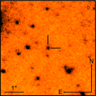
Using the pixel coordinates of the SN in the NOTCAM -band image together with our geometric transformation, we determined the pixel coordinates of the SN in the pre-explosion f/14 image. A source is visible at this position, as can be seen in Figure 16. As before, we measured the position of the source with three different algorithms, taking their standard deviation (1 mas) as the error. The offset between the measured pixel coordinates of the progenitor candidate and the transformed SN pixel coordinates is only 16 mas, well within our combined astrometric uncertainty of 64 mas. We hence find the progenitor candidate to be formally coincident with SN 2012A.
To determine the photometric zero point of the f/14 image, we first photometrically calibrated the f/6 image to the 2MASS system using aperture photometry of two isolated point sources in the field, for which magnitudes were listed in the 2MASS catalog. We then performed aperture photometry on five sources common to both the f/6 and f/14 images, and used these to set the zeropoint of the latter in the 2MASS system. Adding the error from both steps in quadrature, we find an uncertainty of 0.09 mag in the zeropoint of the f/14 image. We performed aperture photometry on the progenitor candidate, and using the determined zeropoint found a magnitude of mag.
For our adopted distance to NGC 3239 ( mag) the progenitor has an absolute magnitude of mag. The foreground extinction ( mag, see Section 4.4) implies an extinction of only 0.01 mag in , with a negligible effect on the progenitor analysis. To determine a progenitor luminosity, we need to know the bolometric correction to the progenitor magnitude. As bolometric corrections vary as a function of temperature (or spectral type), we must assume a temperature range for the progenitor. The fact that SN 2012A is a type IIP SN, with a plateau phase powered by recombination of hydrogen, implies that its progenitor must have been a hydrogen-rich red supergiant. Hence we have taken a range of bolometric corrections to the -band and colours based on synthetic photometry of MARCS model spectra (Gustafsson et al., 2008), appropriate for RSGs with temperatures between 3400 K and 4250 K (Fraser et al. in prep). Over this temperature range, we find that varies between +2.89 mag for the hottest model to +2.29 mag for the coolest.
Applying the average of these values to our progenitor magnitude, we find a bolometric magnitude of mag, where the error is a combination of the photometric error, the uncertainty in the distance, and the range of plausible bolometric corrections. This corresponds to a luminosity of log dex.
To convert the derived luminosity for the progenitor candidate to a mass, we must compare it with the predictions of stellar evolutionary models. We have made this comparison to models from the STARS code (Eldridge et al., 2008 and references therein), which are computed with standard prescriptions for burning, mass loss, overshooting etc. Solar metallicity models were used, although as shown by Smartt et al. (2009b) the precise metallicity has negligible effect on the final luminosity of the models. Smartt et al. also compare the output of the STARS code with other stellar evolutionary codes, and find good agreement.
Comparing the luminosity of the progenitor to the luminosity of stellar evolutionary models at the beginning of core neon burning, we find that a 10.5 M⊙ progenitor is the best match. The lower limit to the luminosity is 4.6 dex, corresponding to a progenitor with a zero-age main sequence mass of 8.5 M⊙. If the progenitor were less massive than this, it would also likely be much more luminous, having undergone second dredge-up, as discussed by Fraser et al. (2011). We set a conservative upper limit to the progenitor mass of 15 M⊙ from comparing the maximum luminosity of the progenitor to the luminosity of the STARS models at the end of core He burning.
The progenitor mass found for SN 2012A, 10.5 M⊙, is comparable to the low progenitor masses found for other type IIP SNe (Smartt, 2009a). We note that the fact that our progenitor detection is in makes it much less sensitive to extinction. As found for SN 2012aw by Fraser et al. (2012) and Van Dyk et al. (2012), and discussed in detail by Kochanek, Khan & Dai (2012), there is evidence that some type IIP SNe have circumstellar dust which is destroyed in the SN explosion, and so the extinction towards the SN cannot be taken as a measure of the extinction towards the progenitor. However, given that the typical extinction of a few magnitudes in seen towards Galactic RSGs by Levesque et al. (2005) would correspond to a few tenths of a magnitude in (a value which is well within our uncertainties), this is not of great concern for this SN.
5.2 Hydrodynamical modeling
An independent approach to constrain the SN 2012A progenitor’s physical properties at the explosion, namely the ejected mass, the progenitor radius and the explosion energy, is through the hydrodynamical modeling of the SN observables, i.e. bolometric light curve, evolution of line velocities and continuum temperature at the photosphere. We adopt the same approach used for other CC SNe (e.g. SNe 2007od, 2009bw, and 2009E; see Inserra et al. 2011, 2012, and Pastorello et al. 2012), in which a simultaneous fit of the observables against model calculations is used.
For computing the models we employ two codes: i) a semi-analytic code (described in detail by Zampieri et al., 2003) which solves the energy balance equation for an envelope with constant density in homologous expansion, and ii) the general-relativistic, radiation-hydrodynamics Lagrangian code presented in Pumo, Zampieri, & Turatto (2010) and Pumo & Zampieri (2011). The latter is able to simulate the evolution of the physical properties of the ejected material and the behavior of the main observables up to the nebular phase, solving the equations of relativistic radiation hydrodynamics for a self-gravitating fluid which interacts with radiation, taking into account both the gravitational effects of the compact remnant and the heating effects linked to the decays of the radioactive isotopes synthesized during the CC SN explosion.
The semi-analytic code is used to perform a preparatory study aimed at individuating the parameter space describing the CC SN progenitor at the explosion and, consequently, to guide the more realistic, but time consuming simulations performed with the general-relativistic, radiation-hydrodynamics code.

In performing the fit, we do not include the observational data taken at phase days that is approximately the time needed for the bolometric light curve to relax to the plateau. At earlier epochs all the observables are significantly affected by emission from the outermost shell of the ejecta (cf. Pumo & Zampieri, 2011). After shock passage, this shell, that contains only a small fraction of the envelope mass, is accelerated to very high velocities and is not in homologous expansion. The structure, evolution and emission properties of this shell cannot be probed in our simulations because at present we adopt an ad hoc initial density profile, not consistently derived from a post-explosion calculation.
In addition, we point out that our modeling is appropriate when the emission from the CC SN is dominated by the expanding ejecta with no contribution from interaction with a dense circumstellar medium (CSM). In fact, as shown by Moriya et al. (2011), the presence of a CSM around the SN (i.e. the remnant of the red supergiant wind) can heavily affect the early evolution of the light curves. In particular, following the collision of the SN ejecta with the CSM, kinetic energy is converted to thermal energy, which is emitted as radiation. As a consequence, the SN appears bright at early times as was observed in SN 2009kf (Botticella et al., 2010). A similar effect may explain the bright initial peak of SN 2012A.
The interaction of the SN ejecta with a CSM can also have signatures either in the radio or in the -ray wavelength regions (cf. for example Chakraborti et al., 2013). As already remarked in Section 3.4, SN 2012A was not detected in the radio domain (Stockdale et al., 2012), while the -ray detection corresponds to a negligible contribution to the bolometric flux (Pooley:2012a). Hence we can safely state that in SN 2012A the contribution from ejecta-CSM interaction to the observed luminosity is negligible.
Based on the adopted explosion epoch (Section 3.1), bolometric luminosity and nickel mass (, Section 5), the best-fitting model shown in Figure 17 has a total (kinetic plus thermal) energy of foe (1 foe erg), initial radius of cm, and envelope mass of . This corresponds to a total stellar mass at the time of explosion of , if we account for a compact remnant. The estimated uncertainty on the total stellar mass is about 15%.
From Figure 17 (middle panel) one can notice a small (10%) systematic offset between the observed photospheric velocity and the modeling. This discrepancy could be reduced, at least for the first two months of evolution, by adopting for the model a slightly higher total energy of foe and an envelope mass between 10 and . However in this case we would get a worse fit to the observed light curve, with a slightly shorter (by about 3 d) plateau.
6 Discussion
SN 2012A is an excellent SN for intensive study thanks to a number of reasons.
Our detailed photometric and spectroscopic optical monitoring, combined with near-infrared photometry and the early photometry from Swift, allow us to reconstruct the evolution of the bolometric luminosity and derive accurate estimates of the expansion velocity and photospheric temperature. From our photometric converge during the radioactive tail of the light curve we could measure a 56Ni mass. Our effort was facilitated by a number of favorable circumstances. Thanks to the high resolution spectra we can derive an accurate estimate of the line of sight extinction, which turned out to be very low. Also, the pre-discovery non-detections and early discovery (in the rising branch of the light curve) allow to constrain the epoch of the explosion, making SN 2012A an ideal case to test hydrodynamic models. Most importantly, thanks to fortuitous deep, high resolution, archival images and the relatively nearby distance to the host galaxy, we could directly identify a progenitor candidate for SN 2012A.
Here we focus on the attempts to constrain the progenitor mass using the two different approaches, namely the direct detection of the progenitor in pre-explosion archival images and the hydrodynamical modeling of the expanding ejecta.
It has been noted that, at least in some cases, the two methods lead to very different results, with the hydrodynamic modeling-derived mass being systematically higher than that obtained from direct measurements (Smartt, 2009a). For instance, through modeling of SN 2005cs and SN 2004et, Utrobin & Chugai (2008, 2009) found progenitor masses of and respectively. These masses are a factor of time larger than the values obtained from an analysis of pre-explosion imaging, and respectively (Smartt et al., 2009b). In other cases the discrepancy is not so large (cf. Table 7 in Maguire et al., 2010b), but always noticeable.
This is also the case for SN 2012A where although the two values are fully consistent within the errors, the best estimate from the hydrodynamic modeling ( including the compact remnant) is about 30% higher that the direct mass estimate ().
Utrobin & Chugai (2009) speculated that hydrodynamic models could overestimate the progenitor mass due to the neglect of multi-dimensional effects. They argued that explosion asymmetries, which are not included in the modeling, may explain the disagreement between progenitor mass determinations for SN 2004et. In that case, a possible bi-polar structure was suggested based on the line profile of the H and [O I] 6300, 6364 Å nebular emissions (Chugai, 2006). A similar feature, namely a double peaked H profile observed in late-stage spectra of SN 2012A (see Section 4.1) could also be an evidence of the asymmetry in the SN ejecta or, most likely, in the radioactive 56Ni bubble.
For direct progenitor detections, a major source of uncertainty is the presence (or absence) of circumstellar dust. In the case of SN 2012aw, Fraser et al. (2012) and Van Dyk et al. (2012) estimated a very low extinction after explosion, but found evidence for pre-existing circumstellar dust which was destroyed in the explosion. For SN 2012A, the possible effect of dust is reduced because the progenitor luminosity was derived from a near-infrared magnitude. A separate source of error arises from the stellar evolutionary models used. As emphasized by Smartt et al. (2009b), a different treatment of mixing processes can change the stellar core mass and hence affect the final luminosity. In particular, the choice of convective overshooting parameter will alter the final configuration of stellar models, with lower overshooting leading to lower luminosity progenitors for a given mass.
As an independent constraint of the progenitor mass, we measured the relative intensities of emission lines in the nebular spectrum and compared these values with the predictions of the spectral synthesis model of Jerkstrand et al. (2012). We found that the [OI] and Na I D line intensities (relative to the total radioactive energy input) are close to the predicted values for a 15 M⊙ star, also consistent with the estimates given above.
In conclusion, all evidence points toward a moderate M⊙ red supergiant star as the progenitor of SN 2012A.
7 Summary
We have presented our extensive data set for SN 2012A, starting from a few days after shock breakout, and covering over one year of evolution to when the SN had completely entered the nebular phase. The collected observations, which consist of photometry, low and high-resolution optical spectroscopy and a near- spectrum, make this type IIP SN one of the most comprehensively observed ever.
The analysis of the observations of SN 2012A show that this is a type IIP supernova with own identity. In particular the plateau appears shorter that in prototypical type IIP SNe, while the plateau luminosity is never really constant. The luminosity in the radioactive tail is moderate, which implies a 56Ni mass which is intermediate between those of prototypical type IIP and faint IIP SNe. In the future, a larger sample of such well studied events exploring the subtle diversity among “normal” SNe IIP, may help to elucidate the details of the explosion mechanism and progenitor properties.
Comparing the bolometric light curve of SN 2012A with that of SN 1987A, we derive for SN 2012A an ejected 56Ni mass of M⊙. This value is intermediate between SN 1999em and the 56Ni-poor SN 2005cs (Pastorello et al., 2009), and close to that of SN 2009bw (Inserra et al., 2012).
The high-resolution spectra allow us to estimate the metallicity of a H II region close to the site of SN 2012A. The estimated oxygen abundance is 12+log(O/H) (using ). The derived metallicity shows that the host of SN 2012A, was in the metal-poor tail of the distribution for the hosts of type II SNe.
A double peaked structure in H profile clearly arises in SN 2012A by day +112 and disappears at around day +173. This may indicate a bipolar structure of the hydrogen excitation and can be interpreted as a result of the asymmetric ejection of 56Ni in the spherically-symmetric envelope (Chugai, 2006).
The direct detection of the progenitor of SN 2012A in archival images indicates that the progenitor star had a moderate mass of 10.5 M⊙. The hydrodynamical modeling of the explosion (bolometric luminosity, Tbb and expansion velocity evolution) and the analysis of [O I] and Na I D nebular lines fluxes (Jerkstrand et al., 2012) seem to favor a slightly higher mass, around 1415 M⊙. Considering the errors on the observables, the assumptions of the evolutionary models, the approximations in the hydrodynamical model, and the uncertainties introduced by a different 56Ni mass for SN 2012A compared to that in the spectral models of Jerkstrand et al. (2012), we find that all three mass estimates are consistent with each other.
Acknowledgments
L.T., E.C., A.P., S.B., F.B. and M.T. are partially supported by the PRIN-INAF 2011 with the project “Transient Universe: from ESO Large to PESSTO”. We acknowledge the TriGrid VL project and the INAF-Astronomical Observatory of Padua for the use of computer facilities. M.L.P. acknowledges the financial support from the PRIN-INAF 2009 “Supernovae Variety and Nucleosynthesis Yields” (P.I. S. Benetti). V.S. acknowledges financial support from Fundação para a Ciência e a Tecnologia (FCT) under program Ciência 2008 and the research grant PTDC/CTE-AST/112582/2009. S.T. acknowledges support by the TRR 33 “The Dark Universe” of the German Research Foundation. G.P. and F.B. acknowledge support from “Millennium Center for Supernova Science” (P10-064-F), with input from “Fondo de Innovación para la Competitividad del Ministerio de Economia, Fomento y Turismo de Chile”. G.P. acknowledges partial support by “Proyecto interno UNAB DI-303-13/R”.
This paper is based on observations collected at the Copernico 1.82m Telescope and Schmidt 67/92 Telescope operated by INAF - Osservatorio Astronomico di Padova at Asiago, Italy, Galileo 1.22m Telescope operated by Department of Physics and Astronomy of the University of Padova at Asiago, Itay. Data was provided by the 2.56m Nordic Optical Telescope operated by The Nordic Optical Telescope Scientific Association (NOTSA), by 2.5 Isaac Newton Telescope and 4.3m William Herschel Telescope operated by the Isaac Newton Group of Telescopes, by the 3.6m Italian Telescopio Nazionale Galileo operated by the Fundación Galileo Galilei - INAF on the island of La Palma. The paper made also use of observations collected at the Observatoire de Haute-Provence 1.93m Telescope operated by Université d’Aix-Marseille and CNRS, France, at the Calar Alto Observatory 2.2m Telescope operated jointly by the Max-Planck-Institut für Astronomie (MPIA) in Heidelberg, Germany, and the Instituto de Astrofísica de Andalucía (CSIC) in Granada/Spain, at NTT, Trappist and REM Telescopes operated by European Southern Observatory (ESO) and Prompt Telescopes operated by Cerro Tololo Inter-American Observatory (CTIO) in Chile.
References
- Anderson et al. (2010) Anderson J. P., Covarrubias R. A., James P. A., Hamuy M., Habergham S. M., 2010, MNRAS, 407, 2660
- Arcavi et al. (2010) Arcavi I., et al., 2010, ApJ, 721, 777
- Asplund et al. (2009) Asplund M., Grevesse N., Sauval A. J., Scott P., 2009, ARA&A, 47, 481
- Barbon et al. (1995) Barbon R., Benetti S., Cappellaro E., Patat F., Turatto M., Iijima T., 1995, A&AS, 110, 513
- Baron et al. (2004) Baron E., Nugent P. E., Branch D., Hauschildt P. H., 2004, ApJ, 616, L91
- Benetti et al. (2001) Benetti S., et al., 2001, MNRAS, 322, 361
- Bersten et al. (2012) Bersten M. C., et al., 2012, ApJ, 757, 31
- Blinnikov et al. (2000) Blinnikov S., Lundqvist P., Bartunov O., Nomoto K., Iwamoto K., 2000, ApJ, 532, 1132
- Botticella et al. (2010) Botticella M. T., et al., 2010, ApJ, 717, L52
- Cardelli, Clayton, & Mathis (1989) Cardelli J. A., Clayton G. C., Mathis J. S., 1989, ApJ, 345, 245
- Chakraborti et al. (2013) Chakraborti S., et al., 2013, arXiv, arXiv:1302.7067
- Chonis & Gaskell (2008) Chonis T. S., Gaskell C. M., 2008, AJ, 135, 264
- Chugai (1991) Chugai N. N., 1991, SvA, 35, 171
- Chugai et al. (2005) Chugai N. N., Fabrika S. N., Sholukhova O. N., Goranskij V. P., Abolmasov P. K., Vlasyuk V. V., 2005, AstL, 31, 792
- Chugai (2006) Chugai N. N., 2006, AstL, 32, 739
- D’Andrea et al. (2010) D’Andrea C. B., et al., 2010, ApJ, 708, 661
- Danziger (1988) Danziger I. J., 1988, snoy.conf, 3
- Dessart & Hillier (2005) Dessart L., Hillier D. J., 2005, A&A, 439, 671
- de Vaucouleurs et al. (1991) de Vaucouleurs G., de Vaucouleurs A., Corwin H. G., Jr., Buta R. J., Paturel G., Fouque P., 1991, S&T, 82, 621
- Eldridge et al. (2008) Eldridge J.J., Izzard R.G., Tout C.A., 2008, MNRAS, 384, 1109
- Elmhamdi et al. (2003a) Elmhamdi A., et al., 2003, MNRAS, 338, 939
- Elmhamdi, Chugai, & Danziger (2003b) Elmhamdi A., Chugai N. N., Danziger I. J., 2003, A&A, 404, 1077
- Falk & Arnett (1977) Falk S. W., Arnett W. D., 1977, ApJS, 33, 515
- Fassia et al. (2001) Fassia A., et al., 2001, MNRAS, 325, 907
- Fitzpatrick (1999) Fitzpatrick E. L., 1999, PASP, 111, 63
- Fraser et al. (2011) Fraser M., Ergon M., Eldridge J.J. et al., 2011, MNRAS, 417, 1417
- Fraser et al. (2012) Fraser M., Maund J.R., Smartt S.J. et al., 2012, ApJ, 759, 13
- Gerardy et al. (2001) Gerardy C. L., et al., 2001, AAS, 33, 1428
- Grassberg, Imshennik, & Nadyozhin (1971) Grassberg E. K., Imshennik V. S., Nadyozhin D. K., 1971, Ap&SS, 10, 28
- Gustafsson et al. (2008) Gustafsson B., Edvardsson B., Eriksson K., Jørgensen U.G., Nordlund Å., Plez B. 2008, A&A 486, 951
- Hamuy et al. (2001) Hamuy M., et al., 2001, ApJ, 558, 615
- Hamuy & Pinto (2002) Hamuy M., Pinto P. A., 2002, ApJ, 566, L63
- Harutyunyan et al. (2008) Harutyunyan A. H., et al., 2008, A&A, 488, 383
- Kochanek, Khan & Dai (2012) Kochanek C.S., Khan R., Dai X., 2012, ApJ, 759, 20
- Hendry et al. (2005) Hendry M. A., et al., 2005, MNRAS, 359, 906
- Hendry et al. (2006) Hendry M. A., et al., 2006, MNRAS, 369, 1303
- Inserra et al. (2011) Inserra C., et al., 2011, MNRAS, 417, 261
- Inserra et al. (2012) Inserra C., et al., 2012, MNRAS, 422, 1122
- Jerkstrand et al. (2012) Jerkstrand A., Fransson C., Maguire K., Smartt S., Ergon M., Spyromilio J., 2012, A&A, 546, A28
- Jones et al. (2009) Jones M. I., et al., 2009, ApJ, 696, 1176
- Landolt (1992) Landolt A. U., 1992, AJ, 104, 340
- Leonard et al. (2002) Leonard D. C., et al., 2002, AJ, 124, 2490
- Leonard et al. (2002) Leonard D. C., et al., 2002, PASP, 114, 35
- Levesque et al. (2005) Levesque E. M., Massey P., Olsen K. A. G., Plez B., Josselin E., Maeder A., Meynet G., 2005, ApJ, 628, 973
- Li et al. (2011) Li W., et al., 2011, MNRAS, 412, 1441
- Litvinova & Nadezhin (1983) Litvinova I. I., Nadezhin D. K., 1983, Ap&SS, 89, 89
- Law et al. (2009) Law N. M., et al., 2009, PASP, 121, 1395
- Maguire et al. (2010a) Maguire K., Kotak R., Smartt S. J., Pastorello A., Hamuy M., Bufano F., 2010, MNRAS, 403, L11
- Maguire et al. (2010b) Maguire K., et al., 2010, MNRAS, 404, 981
- Maguire et al. (2012) Maguire K., et al., 2012, MNRAS, 420, 3451
- Moore et al. (2012) Moore, B., Newton, J., & Puckett, T. 2012, Central Bureau Electronic Telegrams, 2974, 1
- Moriya et al. (2011) Moriya T., Tominaga N., Blinnikov S. I., Baklanov P. V., Sorokina E. I., 2011, MNRAS, 415, 199
- Mould et al. (2000) Mould J. R., et al., 2000, ApJ, 529, 786
- Nugent et al. (2006) Nugent P., et al., 2006, ApJ, 645, 841
- Olivares E. et al. (2010) Olivares E. F., et al., 2010, ApJ, 715, 833
- Osterbrock et al. (2000) Osterbrock D. E., Waters R. T., Barlow T. A., Slanger T. G., Cosby P. C., 2000, PASP, 112, 733
- Otsuka et al. (2012) Otsuka M., et al., 2012, ApJ, 744, 26
- Pastorello et al. (2004) Pastorello A., et al., 2004, MNRAS, 347, 74
- Pastorello et al. (2006) Pastorello A., et al., 2006, MNRAS, 370, 1752
- Pastorello et al. (2009) Pastorello A., et al., 2009, MNRAS, 394, 2266
- Pastorello et al. (2012) Pastorello A., et al., 2012, A&A, 537, A141
- Pettini & Pagel (2004) Pettini M., Pagel B. E. J., 2004, MNRAS, 348, L59
- Phillips & Williams (1991) Phillips M. M., Williams R. E., 1991, supe.conf, 36
- Pooley & Immler (2012) Pooley, D., & Immler, S. 2012, The Astronomer’s Telegram, 3956, 1
- Poznanski et al. (2009) Poznanski D., et al., 2009, ApJ, 694, 1067
- Poznanski, Prochaska, & Bloom (2012) Poznanski D., Prochaska J. X., Bloom J. S., 2012, MNRAS, 426, 1465
- Pozzo et al. (2006) Pozzo M., et al., 2006, MNRAS, 368, 1169
- Prantzos & Boissier (2003) Prantzos N., Boissier S., 2003, A&A, 406, 259
- Prieto, Stanek, & Beacom (2008) Prieto J. L., Stanek K. Z., Beacom J. F., 2008, ApJ, 673, 999
- Prieto et al. (2012) Prieto, J. L., Osip, D., & Palunas, P. 2012, The Astronomer’s Telegram, 3863, 1
- Pritchard et al. (2013) Pritchard, T. A., Roming, P. W. A., Brown, P. J, Bayless, A. J., & Frey, L. H. 2013, arXiv:1303.1190
- Pumo, Zampieri, & Turatto (2010) Pumo M. L., Zampieri L., Turatto M., 2010, MSAIS, 14, 123
- Pumo & Zampieri (2011) Pumo M. L., Zampieri L., 2011, ApJ, 741, 41
- Quimby et al. (2007) Quimby R. M., Wheeler J. C., Höflich P., Akerlof C. W., Brown P. J., Rykoff E. S., 2007, ApJ, 666, 1093
- Sanders et al. (2012) Sanders N. E., et al., 2012, ApJ, 758, 132
- Schmidt, Kirshner, & Eastman (1992) Schmidt B. P., Kirshner R. P., Eastman R. G., 1992, ApJ, 395, 366
- Schlafly & Finkbeiner (2011) Schlafly E. F., Finkbeiner D. P., 2011, ApJ, 737, 103
- Schlegel, Finkbeiner, & Davis (1998) Schlegel D. J., Finkbeiner D. P., Davis M., 1998, ApJ, 500, 525
- Stockdale et al. (2012) Stockdale, C. J., Ryder, S. D., Van Dyk, S. D., et al. 2012, The Astronomer’s Telegram, 3861, 1
- Smartt (2009a) Smartt S. J., 2009, ARA&A, 47, 63
- Smartt et al. (2009b) Smartt S. J., Eldridge J. J., Crockett R. M., Maund J. R., 2009, MNRAS, 395, 1409
- Stanishev & Pursimo (2012) Stanishev, V., & Pursimo, T. 2012, Central Bureau Electronic Telegrams, 2974, 3
- Stoll et al. (2012) Stoll R., Prieto J. L., Stanek K. Z., Pogge R. W., 2012, arXiv, arXiv:1205.2338
- Tully (1988) Tully R. B., 1988, ngc..book,
- Tully et al. (2009) Tully R. B., Rizzi L., Shaya E. J., Courtois H. M., Makarov D. I., Jacobs B. A., 2009, AJ, 138, 323
- Turatto et al. (1993) Turatto M., Cappellaro E., Benetti S., Danziger I. J., 1993, MNRAS, 265, 471
- Turatto et al. (1998) Turatto M., et al., 1998, ApJ, 498, L129
- Utrobin (2007) Utrobin V. P., 2007, A&A, 461, 233
- Utrobin, Chugai, & Pastorello (2007) Utrobin V. P., Chugai N. N., Pastorello A., 2007, A&A, 475, 973
- Utrobin & Chugai (2008) Utrobin V. P., Chugai N. N., 2008, A&A, 491, 507
- Utrobin & Chugai (2009) Utrobin V. P., Chugai N. N., 2009, A&A, 506, 829
- Van Dyk et al. (2012) Van Dyk S.D., Cenko S.B., Poznanski D. et al., 2012, ApJ, 756, 131
- Walmswell & Eldridge (2012) Walmswell J. J., Eldridge J. J., 2012, MNRAS, 419, 2054
- Woosley, Hartmann, & Pinto (1989) Woosley S. E., Hartmann D., Pinto P. A., 1989, ApJ, 346, 395
- Zampieri et al. (2003) Zampieri L., Pastorello A., Turatto M., Cappellaro E., Benetti S., Altavilla G., Mazzali P., Hamuy M., 2003, MNRAS, 338, 711
- Zampieri (2007) Zampieri L., 2007, AIPC, 924, 358