A Calculus for Higher Spin Interactions

Abstract

Higher spin theories can be efficiently described in terms of auxiliary Stückelberg or projective space field multiplets. By considering how higher spin models couple to scale, these approaches can be unified in a conformal geometry/tractor calculus framework. We review these methods and apply them to higher spin vertices to obtain a generating function for massless, massive and partially massless three-point interactions.

1 Introduction

Massless and massive higher-spin interactions are believed to be governed by Vasiliev’s equations [1] and by String Theory, respectively; relating these theories is a pressing problem for modern theoretical physics. For the former, scattering amplitudes are formulated as ($d=2$) CFT vertex operator correlators while the Vasiliev system relies on an unfolded frame-like approach. However, in the end, one is often interested in either an $S$-matrix or Witten-type diagrams, whose features can often be determined by gauge invariance alone. In a light-cone framework and flat backgrounds, detailed results for massless [2, 3, 4] and massive [5, 6] cubic higher spin interactions were obtained by following exactly this philosophy. More recently, a covariant version of this program was carried out for higher spin cubic vertices, both for simple cases (see, for example [7, 8, 9, 10, 11, 12] and the review [13]) and rather generally [14, 15, 16, 17]. The (anti) de Sitter [(A)dS] and general mass (including partially massless [PM]) cases were then given in [18, 19, 20, 21, 22, 23], while frame-like and mixed symmetry analyses were performed in [24, 25] and [26, 27, 28, 29], respectively. Early results beyond cubic order are available in both light-cone formalism [30, 31] and covariant settings [32, 33, 34].

A central difficulty faced by higher spin theories is maintaining correct degrees of freedom (DoF) counts in the presence of interactions which generically destroy the gauge invariances or constraints controlling the DoF of free higher spin wave equations. For non-interacting theories, by including Stückelberg auxiliary fields, gauge invariance can be used as the central principle underlying the propagating higher spin DoF for all mass types: There are various ways to understand the auxiliary field content required for massive higher spin fields, crucial among them being their origin as Scherk–Schwarz reductions [35] of massless higher spins in one higher dimension [36, 37]. Indeed, by a radial reduction corresponding to a conformal isometry of a flat embedding space [38], the same mechanism generates the Stückelberg couplings for higher spins in constant curvature backgrounds [39]. This is the first hint that conformal geometry might play a rôle in these constructions. It also suggests an underlying Dirac space construction, where conformally flat spaces are realized as sections of a cone in two higher dimensions. What is surprising is that such methods, which have long been known to be applicable to models with conformal symmetries [40], can actually be used to great advantage for massive—non-conformal—models [41, 42, 43].

The flat model for a $d$-dimensional conformal geometry is obtained by sections of an ambient light-cone in $(d+2)$-dimensions. Metrics induced on $d$-dimensional slices by the $(d+2)$-dimensional ambient metric are conformally related. Metrics induced by flat slices (the classical conic sections) give constant curvature spaces, as depicted in Figure 1.

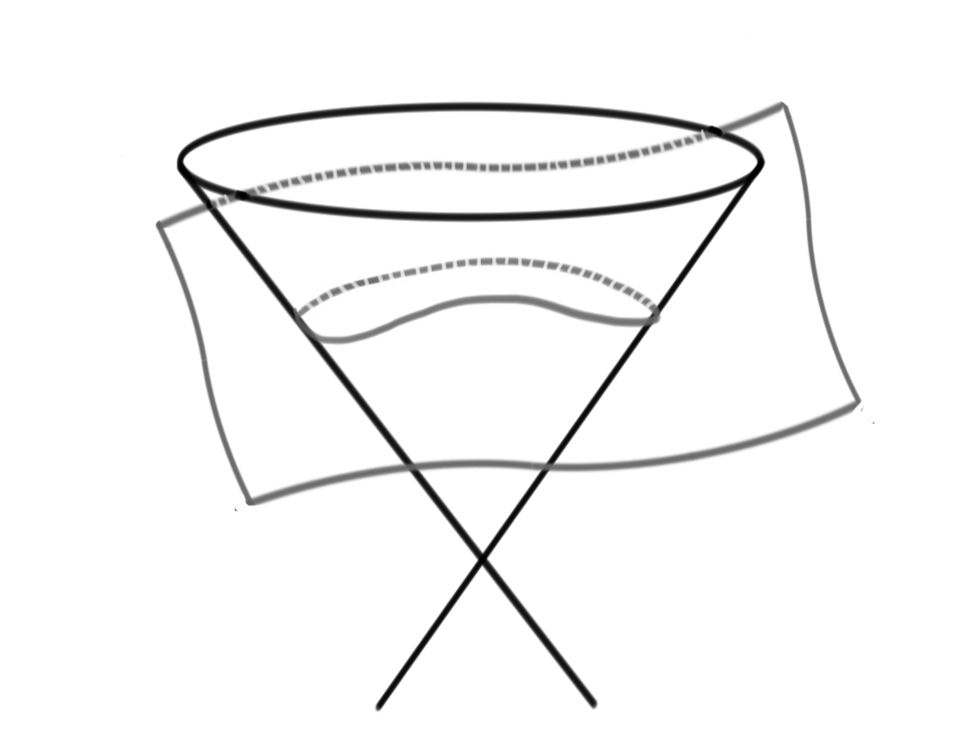
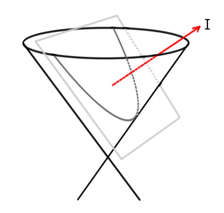
Figure 1: Conformally related metrics are obtained by slicing the conformal cone. These are conformally Einstein when there exist slices admitting a parallel scale tractor $I$. The second picture depicts the slice inducing an Einstein metric.

These are characterized by the normal vector $I$—which we will later elevate to a parallel ambient vector field termed the scale tractor—to the flat slicing hypersurface. Moreover this flat model can be generalized to the curved setting where the space of slicings yields general conformal classes of metrics, while parallel scale tractors correspond to Einstein metrics. So in this picture, solving Einstein’s equations amounts to finding parallel scale tractors [44].

The relevance of a six dimensional cone to four dimensional conformal wave equations was first observed by Dirac [40] while its $(d+2)$-dimensional curved generalization and application to $d$-dimensional conformal geometry was initiated by Fefferman and Graham [45]. The parallel scale tractor description of conformally Einstein metrics was discovered by Bailey, Eastwood and Gover in a paper which also developed the so-called ($d$-dimensional) “tractor calculus” for conformal invariants [44]. Later it was realized that tractors could also be profitably described using ambient $(d+2)$-dimensional tensors [46, 47]. Moreover, it was shown that tractors could be used to express the fundamental wave equations of physics [41, 42, 43]. The main idea was very simple: while parallel scale tractors $I$ describe the background Einstein geometry, evolving boundary data along $I$ corresponds to wave equations. This development allowed both massless and massive wave equations to be described by conformal geometry, rather than Riemannian geometry methods. Mass then amounts to how physical fields respond to changes of scale (i.e., their tractorial weights).

The above picture becomes much richer when one considers also boundary problems, in particular those with data at conformal infinities. In fact, this is precisely the setting of the AdS/CFT correspondence [48, 49]. Firstly, the slicing hypersurface is described by the constant locus of a unit homogeneity scalar called the scale $\sigma$, that plays the rôle of a dilaton field, or in other words a $d$-dimensional scalar, conformal density. A key insight of Gover [50], was that although a nowhere-vanishing scale and a conformal class of metrics is equivalent to a Riemannian geometry, this is not the case when $\sigma$ has a non-trivial zero-locus. This led to a generalization called “almost Riemannian geometry”. In hyperbolic settings the zero locus of the scale $\sigma$ amounts to a conformal infinity. This is depicted in the conformally flat—conic sections—setting in Figure 2.

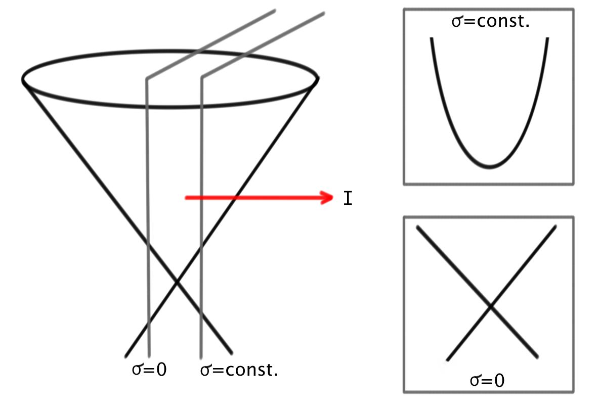
Figure 2: Coupling to scale through the scale tractor $I$ determines the evolution of physical fields with masses labeled by conformal weights. The scale tractor also determines how data is moved from the boundary (the zero scale slice) to the bulk (standardly described by a constant scale slice).

Observe that constant loci of $\sigma$ intersect the cone along hyperboloids (positively curved constant curvature spaces) while the zero locus yields a cone, and in turn conformal structure, in one dimension less. The former intersection corresponds to the bulk manifold in an AdS/CFT correspondence while the latter yields the boundary conformal geometry (and in turn CFT).

The power of this approach is that the bulk conformal structure can be utilized to realize spectrum or solution generating symmetries [48, 49]: The contraction of the scale tractor $I$ with a tractor analog of the gradient and Laplace operators (known as the Thomas-$D$ operator [44]) yields the so-called Laplace-Robin operator. This is a conformal version of the bulk Laplacian which continues smoothly to the boundary (even though it is at conformal infinity). Remarkably, this operator is a generator of an ${\mathfrak{s}l}(2)$ solution-generating algebra valid on any curved manifold [48]. This facilitates solutions to conformal infinity boundary problems. These results have a wide applicability, both to higher spin, bose, fermi, massless, massive and PM systems. Hence, the main building blocks for a calculus for scattering problems taking full advantage of the bulk conformal structure are now available. The next (and crucial) step is to describe higher spin vertices in this approach. In this article we show how this can be done for totally symmetric higher spin fields. This requires a melding of known results for these vertices with tractor approaches to higher spin fields.

Before summarizing our results, we provide a brief guide to the Article. In Section 2 we review the tractor calculus description of conformal geometry and of physical systems in terms of conformally invariant tractors coupled to scale. In Section 3 we specialize these methods to higher spins, focusing on their on-shell description. The results in Section 3.2 focus on how to write point-split on-shell amplitudes (à la [15, 16, 18, 19, 20, 21, 23]) in terms of tractor multiplets and are new. In Section 4 we apply our “tractor higher spin Noether method” to compute the three point vertex generating functions. In the Appendices, we derive various key identities and connect our results with previous ones based on a $(d+1)$-dimensional projective space approach [18, 19, 20, 21, 23].

Summary of results

Our results for totally symmetric higher spins of arbitrary rank can be compactly expressed in terms of tractor generating functions $\Phi(x,U)$ (where a $(d+2)$-dimensional auxiliary vector $U^{M}$ is used to keep track of tractor bundle valued indices–see Section 3.1). Vertex generating functions can be expressed in terms of the irreducible set of operators

$${\mathcal{Y}}_{i}=\partial_{U_{i}}\cdot\widehat{D}_{i+1}\,,\qquad{\mathcal{Z}}_{i}=\sigma^{-2}\,\partial_{U_{i-1}}\!\!\cdot\partial_{U_{i+1}}\qquad[i\simeq i+3]\,,$$

built from the Thomas-$D$ operator (see Section 3.2):

$$S^{\scriptscriptstyle(3)}\sim\int_{\sigma}\,\scalebox{1.2}{:}\,\sigma^{\sum_{i}\tau_{i}}\,C({\mathcal{Y}}_{i}\,,{\mathcal{Z}}_{i})\,\scalebox{1.2}{:}\,\Phi(X_{1},U_{1})\,\Phi(X_{2},U_{2})\,\Phi(X_{3},U_{3})\,\Big{|}_{\overset{x_{i}=x}{\scriptscriptstyle U_{i}=0}}\,.$$

Here, the integration measure $\int_{\sigma}$ is defined in (3.4), the normal ordering is $\sigma>{\mathcal{Y}}>{\mathcal{Z}}$ and the parameters $\tau_{i}$ are the twists of respective fields. Our punchline is a proof that the tractor gauge consistency condition–which amounts to (strictly) massless ($\tau_{1}=2$) gauge transformations in a dual $(d+2)$-dimensional theory [41, 42, 51], gives a differential equation determining the function $C$ :

$$\Big{[}{\mathcal{Y}}_{3}\partial_{{\mathcal{Z}}_{2}}-{\mathcal{Y}}_{2}\partial_{{\mathcal{Z}}_{3}}\,-\hat{\gamma}\left({\mathcal{Y}}_{3}\partial_{{\mathcal{Y}}_{3}}-{\mathcal{Y}}_{2}\partial_{{\mathcal{Y}}_{2}}+\tfrac{\tau_{2}-\tau_{3}}{2}\right)\partial_{{\mathcal{Y}}_{1}}\Big{]}\,C(\,{\mathcal{Y}}_{i}\,,\,{\mathcal{Z}}_{i}\,)\,=\,0\,,$$ (1.1)

where

$$\hat{\gamma}=\tau_{2}+\tau_{3}-d+1-2\,\sum_{i}{\mathcal{Z}}_{i}\partial_{{\mathcal{Z}}_{i}}\,.$$

This equation has already been solved in [23]: For that one absorbs the factor $-\,\hat{\gamma}$ into a differential operator $\hat{\delta}$

$$\hat{\delta}\,=\,-\sigma^{d}\,\frac{d}{d\sigma}\,\sigma^{-d+1}\,.$$

Exactly the same operator arose in [20] from a careful handling of a projective space delta function measure. In these terms, the cubic coupling for three massless fields can be written as

$$C(\,{\mathcal{Y}}_{i}\,,\,{\mathcal{Z}}_{i}\,)\,=\,e^{-\,\hat{\delta}\,{\cal D}}\,K(\,{\mathcal{Y}}_{i}\,,\,{\cal G}\,)\,\big{|}_{{\cal G}=\sum_{i}{\mathcal{Y}}_{i}\,{\mathcal{Z}}_{i}}\,,$$

where ${\cal D}:=\big{[}{\mathcal{Z}}_{1}\partial_{{\mathcal{Y}}_{2}}\partial_{{\mathcal{Y}}_{3}}+{\mathcal{Z}}_{1}{\mathcal{Z}}_{2}\partial_{{\mathcal{Y}}_{3}}\partial_{{\cal G}}+\text{cyclic}\big{]}+{\mathcal{Z}}_{1}{\mathcal{Z}}_{2}{\mathcal{Z}}_{3}\,\partial_{{\cal G}}^{2}$ (see [20, 23]) and $K$ is an arbitrary polynomial function of four variables.

The same pattern arises also for generic massive and (partially-)massless couplings. These correspond to various intersections of kernels of the differential operator appearing in Eq. (1.1), and cyclic permutations thereof, as discussed in [23]. In summary, we find that the solutions in the projective formalism of [23] and the corresponding tractor ones are related simply by replacing the $(d+1)$-dimensional integration with the standard (conformally invariant) $d$-dimensional measure along with substitutions $Y\rightarrow{\mathcal{Y}}$ and $Z\rightarrow{\mathcal{Z}}$. In particular, the tractor approach gives an alternative proof of the $\delta$-function methods used in [18, 19, 20, 21, 23].

2 Tractors

A conformal $d$-manifold ${\cal M}$ is a manifold equipped with a conformal class of metrics $[g_{\mu\nu}]=[\Omega^{2}\,g_{\mu\nu}]$. The data $({\cal M},[g])$ determines the standard tractor bundle ${\cal T}{\cal M}$ over ${\cal M}$, which can be viewed as a conformally invariant extension of the tangent bundle $T{\cal M}$. This comes equipped with a canonical tractor connection $\nabla^{\cal T}$. In simple (four dimensional-)terms, tractors replace four-vectors (sections of $T{\cal M}$) by six-vector sections of ${\cal T}{\cal M}$ in order to make Weyl invariance manifest. Under changes of Weyl frame $g_{\mu\nu}(x)\mapsto\Omega^{2}(x)\,g_{\mu\nu}(x)$, a standard tractor $V^{M}\in\Gamma{\cal T}{\cal M}$ ($M=0,\ldots,d+1$) transforms as

$$V^{M}:=\begin{pmatrix}V^{+}\\ V^{m}\\ V^{-}\end{pmatrix}\longmapsto\begin{pmatrix}\Omega V^{+}\\ V^{m}+\Upsilon^{m}V^{+}\\ \Omega^{-1}\big{(}V^{-}-\Upsilon_{\mu}V^{\mu}+\frac{1}{2}\Upsilon^{2}V^{+}\big{)}\end{pmatrix}=:U^{M}{}_{N}V^{N}\,.$$

Here $\Upsilon_{\mu}:=\Omega^{-1}\partial_{\mu}\Omega$ and we have used the vielbein in the middle slot to flatten indices. The matrix $U^{M}{}_{N}$ is $SO(d+1,1)$-valued. The tractor connection acts on $V^{M}$ as

$$\nabla_{\mu}^{\cal T}V^{M}=\begin{pmatrix}\partial_{\mu}V^{+}-V_{\mu}\\ \nabla_{\mu}V^{m}+e_{\mu}{}^{m}V^{+}+{\mbox{\sf P}}_{\mu}{}^{m}V^{-}\\ \partial_{\mu}V_{-}-{\mbox{\sf P}}_{\mu}{}^{m}V_{m}\end{pmatrix}\,,$$

and is the covariant derivative with respect to the change of Weyl frame given above. On the right hand side of this formula, $\nabla$ denotes the Levi-Civita connection and the Schouten tensor ${\mbox{\sf P}}_{\mu\nu}$ is defined by the decomposition of the Riemann tensor into its trace-free Weyl plus trace pieces:

$$R_{\mu\nu\rho\sigma}=W_{\mu\nu\rho\sigma}+g_{\mu\rho}{\mbox{\sf P}}_{\nu\sigma}-g_{\nu\rho}{\mbox{\sf P}}_{\mu\sigma}+g_{\nu\sigma}{\mbox{\sf P}}_{\mu\rho}-g_{\mu\sigma}{\mbox{\sf P}}_{\nu\rho}\,.$$

To complete the tractor calculus we introduce weighted tractors $V^{M}\in\Gamma{\cal T}{\cal M}[w]$ transforming as

$$V^{M}\mapsto\Omega^{w}\,U^{M}{}_{N}V^{N}\,,$$

as well as a pair of tractor operators, of weights $-1$ and $+1$, respectively known as the Thomas-$D$ operator and canonical tractor:

$$D^{M}:=\begin{pmatrix}w(d+2w-2)\\ (d+2w-2)\nabla^{m}\\ -\Delta-w{\mbox{\sf J}}\end{pmatrix}\quad\mbox{and}\qquad X^{M}=\begin{pmatrix}0\\ 0\\ 1\end{pmatrix}\,.$$

These both act on (weighted) tractor(-tensor)s yielding tractor(-tensor)s, for this reason we have dropped the (implicit) label ${\cal T}$ on the tractor connection, also $\Delta:=g^{\mu\nu}\nabla_{\mu}\nabla_{\nu}$ and ${\mbox{\sf J}}:={\mbox{\sf P}}^{\mu}_{\mu}$. Importantly, for any conformal structure $({\cal M},[g_{\mu\nu}])$, these operators obey a null condition $D_{M}D^{M}=0=X^{M}X_{M}\,$, where indices are raised and lowered with the $SO(d+1,1)$-invariant tractor metric $V\cdot V^{\prime}:=V^{+}V^{\prime}{}^{-}+V^{-}V^{\prime}{}^{+}+V^{m}V^{\prime}_{m}$ .

Since the Thomas-$D$ operator unifies the Laplacian and gradient operators in a single tractor multiplet of operators, it will play a crucial rôle in many computations. Let us gather together some of its key properties: Firstly, it is null, in the sense:

$$D_{M}D^{M}=0\,.$$

However, since it is second order in derivatives, it does not obey a Leibniz rule. Nonetheless, an integration by parts formula does hold (with an unusual sign)

$$\int_{{\cal M}}\!d^{d}x\,\sqrt{-g}\ V^{M}\,D_{M}U=\int_{{\cal M}}\!d^{d}x\,\sqrt{-g}\ (D_{M}V^{M})\,U\,,$$ (2.1)

for any tractors $V^{M}$ and $U$ (suppressing further indices such that the overall integrand is a scalar) of weights $w_{V}$ and $w_{U}$ subject to $d+w_{V}+w_{U}-1=0$ (which ensures that the integrand is of zero weight). Moreover, the failure of the Leibniz property can be characterized as follows: Acting on any tractor with weight $w\neq 1-\frac{d}{2}$ we first define

$$\widehat{D}^{M}:=\frac{1}{d+2w-2}\,D^{M}\,.$$

Then if  $A$ and $B$ are tractors of weight $w_{A}$ and $w_{B}$, respectively, the failure of the Leibniz rule is measured by the following identity

$$\widehat{D}^{M}(AB)-(\widehat{D}^{M}A)B-A(\widehat{D}^{M}B)=-\frac{2}{d+2w_{A}+2w_{B}-2}\,X^{M}(\widehat{D}^{N}A)(\widehat{D}_{N}B)\,.$$ (2.2)

This is easily verified by using the ambient formula for the Thomas-$D$ operator given in (2.5) below, and is valid away from obvious poles at distinguished values of $w_{A},w_{B}$. This formula can be further simplified to an operator statement by introducing the weight operator $h$ whose eigenvalue is $d+2w$ acting on weight $w$ tractors:

$$\widehat{D}^{M}A-(\widehat{D}^{M}A)-A\,\widehat{D}^{M}=-\frac{2}{h}\,X^{M}(\widehat{D}^{N}A)\,\widehat{D}_{N}\,.$$

From time to time, we will need the commutator between the Thomas-$D$ and canonical tractor operators:

$$\left[X^{M}\,,\,\widehat{D}^{N}\right]\,=\,\frac{2}{h}\,X^{N}\,\widehat{D}^{M}\,-\,\eta^{MN}\,,\qquad\eta_{MN}=\begin{pmatrix}0&0&1\\ 0&\eta_{mn}&0\\ 1&0&0\end{pmatrix}\,,$$ (2.3)

where $\eta_{MN}$ is the $SO(d,2)$-invariant metric.

Finally, on conformally Einstein manifolds, the Thomas-$D$ operator commutes with the scale tractor $I_{M}=\widehat{D}_{M}\,\sigma$ (see Section 2.2):

$$\left[D^{M}\,,\,I^{N}\right]\,=\,0\,,\qquad[\widehat{D}^{M}\,,\,I^{N}]\,=\,0\,,$$

while it commutes with itself on flat conformal structures:

$$[\,D^{M}\,,\,D^{N}\,]=0\,,\qquad[\,\widehat{D}^{M}\,,\,\widehat{D}^{N}\,]=0\,.$$

2.1 Ambient tractors

The bundle-theoretic description of tractors and their calculus is extremely useful for computations whose output is required in standard Riemannian geometry terms. However, for many computations, an ambient description of tractors is very powerful. For that we first introduce a Fefferman–Graham ambient space. This is a $(d+2)$-dimensional space $\widetilde{\cal M}$ endowed with a metric obeying

$$G_{MN}=\nabla_{M}X_{N}$$

for some vector field $X_{N}$. This condition immediately implies $G_{MN}=\frac{1}{2}\nabla_{M}\partial_{N}X^{2}$. The function $X^{2}$ is known as a homothetic potential or a defining function; its zero locus defines a curved version of the Dirac cone described and depicted in the Introduction. The transition to the underlying $d$-dimensional conformal geometry is achieved via reducing to the cone and then demanding a homogeneity condition with respect to the homothety $X^{M}$. More precisely, tractor(-tensor)s are equivalence classes of ambient tensors on $(\widetilde{\cal M},G_{MN})$

$$T^{M_{1}\cdots M_{s}}\sim T^{M_{1}\cdots M_{s}}+X^{2}\,S^{M_{1}\cdots M_{s}}\,,$$ (2.4)

(where the tensor $S$ extends smoothly to the cone $\{X^{2}=0\}$; spinor-tractors can be defined analogously [43]) classified by weights $w$

$$X\cdot\nabla\,T^{M_{1}\cdots M_{s}}=w\,T^{M_{1}\cdots M_{s}}\,.$$

The equivalence relation (2.4) is precisely that enjoyed by the lightlike physical excitations of a massless scalar field in a momentum basis. Therefore, tractor operators can be derived by considering the momentum representation of the $\mathfrak{so}(d+2,2)$ generators of the conformal group acting on a flat ambient space [51]. Their generally curved counterparts follow by replacement of partial derivatives by covariant ones. Thus, acting on ambiently represented tractors, the Thomas-$D$ operator is given by the analog of a momentum space conformal boost

$$D_{M}=(d+2\,X\cdot\nabla)\,\nabla_{M}-X_{M}\,\nabla^{2}\,.$$ (2.5)

This construction ensures that $D_{M}$ respects the equivalence relation (2.4).

2.2 Wave equations

To describe the evolution of physical fields we must consider how they couple to scale. This problem is solved by first considering gravity. To begin with, suppose we are given a double conformal class of a metric and scale $[g_{\mu\nu},\sigma]=[\Omega^{2}\,g_{\mu\nu},\Omega\,\sigma]$. From this we can construct the scale tractor $I_{M}=\frac{1}{d}\,D_{M}\sigma=\begin{pmatrix}-\frac{1}{2}(\Delta\sigma+{\mbox{\sf J}}\sigma),&n_{m},&\sigma\end{pmatrix}$, where $n_{\mu}:=\partial_{\mu}\sigma$. Requiring that $I^{M}$ is tractor parallel

$$\nabla^{\cal T}_{\mu}I^{M}=0\,,$$

ensures that $g_{\mu\nu}$ is conformal to an Einstein metric, with the Einstein metric being achieved precisely in the choice of Weyl frame $\sigma={\rm constant}$. This is the mathematics behind the conic sections picture of Einstein geometries sketched in the Introduction. Moreover, since $I^{M}$ is parallel for conformally Einstein metrics, its square $I^{2}=I^{M}I_{M}$ is constant; physically this is the cosmological constant. Note that the Einstein–Hilbert action in these terms is simply the conformally invariant expression $S[g,\sigma]=\int d^{d}x\sqrt{-g}\,\sigma^{-d}I^{2}$, so that Einstein’s equations amount to extremizing the magnitude of the scale tractor (a cosmological term is just the integral of the conformally invariant measure: $\int d^{d}x\sqrt{-g}\,\sigma^{-d}$.) In fact, taking the normal vector $n_{\mu}=\partial_{\mu}\sigma$ to loci of constant $\sigma$ as an independent field, then the pair $(\sigma,n_{\mu})$ can be viewed as a generalized lapse and shift and thus the parallel scale tractor equation yields a covariant extension of the ADM formalism.

Not only does the scale tractor control the geometry, it determines the evolution of physical fields. If $\Phi^{\bullet}$ is any tractor tensor, the quantity $D^{M}\Phi^{\bullet}$ is covariant under Weyl transformations. Generally, wave equations are not conformally invariant, so they must somehow be coupled to scale. There is a simple universal prescription for this, namely the contraction with the scale tractor

$$I_{M}D^{M}\Phi^{\bullet}=0\,.$$

The operator $I\cdot D:=I_{M}D^{M}$ is called the Laplace-Robin operator because in the bulk it is a conformally invariant version of the Laplacian while along the boundary it gives the Robin operator, which is a conformally invariant normal derivative [52]. Crucially, the operator $I\cdot D$ extends smoothly to conformal infinities encoded by the zero locus of the scale $\sigma=0$. From the conical section picture of the Introduction and the interpretation of the Thomas-$D$ operator as the generalization of the ambient gradient operator, it follows that the Laplace-Robin operator generates evolution along the $\sigma$-direction, indeed this underlies standard Fefferman-Graham type expansions of the type crucial to the AdS/CFT correspondence [48, 42]. Also, it is important to note that the weight of the tractor $\Phi^{\bullet}$ will encode the mass of its underlying physical excitations [41], indeed the general mass Weyl-weight relationship for spin $s$ fields is given by

$$m^{2}=-\frac{2{\mbox{\sf J}}}{d}\,(w-s+2)(d+w+s-3)\,,$$ (2.6)

where for constant curvature spaces $\frac{\scalebox{0.7}{{\mbox{\sf J}}}\,\!}{d}=\frac{\Lambda}{(d-1)(d-2)}$. Massless fields appear when $w=s-2$ while depth $t$ PM ones arise at $w=s-t-1$  (maximal depth $t=s$ PM fields always have $w=-1$).

Generally for higher spins, we are not interested in wave equations alone, but must augment these with transversality conditions. The first point to notice, is that as the spin increases, consistency of transversality requirements impose restrictions on the backgrounds in which higher spin fields can propagate. We do not wish to delve further into that issue here, so for the remainder of this discussion concentrate on conformally flat spaces. This has the happy consequence that commutators of the Thomas-$D$ operator and scale tractor vanish $[D^{M},D^{N}]=0=[D^{M},I^{N}]$ (the latter of these conditions of course holds more generally in conformally Einstein spaces). Also, for massive spins, we desire a simple calculus automatically incorporating the Stückelberg fields required to describe them in a gauge invariant way. Let us sketch how this works for spins 1 and 2 before giving the equations we need at general $s$ in Section 3. For spin 1 we take as field content a weight $w$ tractor $A_{M}$ while for spin 2 we consider a weight $w$ rank 2 symmetric tractor $h_{MN}$ and postulate gauge invariances mimicking their Maxwell and linearized general coordinate counterparts

$$\delta A_{M}=D_{M}\alpha\,,\qquad\delta h_{MN}=D_{M}\xi_{N}+D_{N}\xi_{M}\,.$$

Because the Thomas-$D$ operator is null, under these transformations the “Feynman- and Fock-de Donder-gauge” parts of the fields $A_{M}$ and $h_{MN}$ are, respectively, gauge inert, thus we may consistently impose conditions

$$D^{N}A_{N}=0\,,\qquad D^{M}h_{MN}-\frac{1}{2}D_{M}h_{N}^{N}=0\,.$$ (2.7)

These conditions already ensure that the tractors $A_{M}$ and $h_{MN}$ are parameterized by: a vector and Stückelberg scalar for the Maxwell case; and metric fluctuations and a Stückelberg vector and scalar for the spin 2 case. For example, in the spin 2 case one finds gauge transformations for the metric fluctuations $h_{\mu\nu}$ and Stückelberg fields $(V_{\mu},\varphi)$ [41, 42]

$$\delta h_{\mu\nu}=\nabla_{(\mu}\xi_{\nu)}+\frac{2\scalebox{1.0}{{\mbox{\sf J}}}}{d}\,g_{\mu\nu}\,\xi\,,\quad\delta V_{\mu}=w\,\xi_{\mu}+\partial_{\mu}\xi\,,\quad\delta\varphi=(w+1)\,\xi\,.$$

For generic weights (and in turn $w$), the Stückelberg fields can be gauged away leaving a massive theory for $h_{\mu\nu}$; when $w=0$, the Stückelberg scalar $\varphi$ can be gauged away and the vector $V_{\mu}$ decouples leaving massless metric fluctuations $h_{\mu\nu}$ with a linearized diffeomorphism gauge symmetry $\delta h_{\mu\nu}=\nabla_{(\mu}\xi_{\nu)}$. At $w=-1$, the scalar decouples and the vector Stückelberg mode can be gauged away leaving residual symmetries with $\xi_{\mu}=\partial_{\mu}\xi$. Under these, the metric fluctuations enjoy the PM gauge symmetry $\delta h_{\mu\nu}=\big{(}\nabla_{\mu}\partial_{\nu}+\frac{2\scalebox{0.7}{{\mbox{\sf J}}}}{d}\,g_{\mu\nu}\big{)}\xi$.

Oftentimes, a $(d+1)$-dimensional projective approach based on a log-radial reduction [38] is employed to describe massive higher spins. In fact the above Stückelberg gauge transformations can be derived exactly in that way [39]. In the above description, the independent tractor field content is given by components $h^{++},h^{+m}$ and $h^{mn}$. In fact quite generally, the “top slots” of tractor fields encode the $(d+1)$-dimensional projective construction [42]. Geometrically this is easy to see; essentially one is projecting the Dirac cone along the scale tractor onto a surface of constant $\sigma$. The images of conical sections at fixed values of $\sigma$ are mapped in this way to loci with constant values of the log-radial coordinate in a $(d+1)$-dimensional hypersurface. These loci are again constant curvature manifolds.

The equations of motion for spins 1 and 2 are given by forming tractor analogs of the Maxwell curvature and Christoffel symbols

$$F_{MN}:=D_{M}A_{N}-D_{N}A_{M}\,,\qquad\Gamma^{R}_{MN}:=D_{(M}^{\phantom{R}}h^{R}_{N)}-\frac{1}{2}D^{R}h_{MN}\,,$$

and then coupling these to scale by simply contracting with the scale tractor

$$I^{M}F_{MN}=0\,,\qquad I_{R}^{\phantom{R}}\Gamma^{R}_{MN}=0\,.\qquad$$ (2.8)

These equations of motion enjoy the above gauge invariances (so long as $I_{M}\xi^{M}=0$ for spin 2) and have as leading terms the universal Laplace-Robin structure $I\cdot D\,A_{M}+\cdots=0$,  $I\cdot D\,h_{MN}+\cdots=0$. They encode massive, massless and PM equations in a unified framework.

3 Tractors and higher spins

In this Section we apply tractor technology to higher spin fields. In particular we show how to write wave equations and then construct on-shell vertex functionals.

3.1 On-shell higher spin tractors

For our “on-shell” purposes, the off-shell equations of motion presented for the special case of spin $s=1,2$ cases in the previous section are not optimal. Their on-shell counterparts are obtained by fixing gauges for the Stückelberg auxiliaries:

$$X^{M}\Phi_{MM_{2}\cdots M_{s}}=0\,,\qquad I^{M}\Phi_{MM_{2}\cdots M_{s}}=0\,,\qquad\Phi^{M}{}_{MM_{3}\cdots M_{s}}=0\,.$$

We then obtain the following equations, which generalize (2.7) and (2.8) directly to their higher $s$ counterparts:

$$D^{M}\Phi_{MM_{2}\cdots M_{s}}=0\,,\qquad I\cdot D\,\Phi_{M_{1}\cdots M_{s}}=0\,.$$ (3.1)

Here, $\Phi_{M_{1}\ldots M_{s}}$ is a totally symmetric weight $w$ tractor, and masses and weights are related by (2.6) above. For tuned weights

$$w=-1,0,\ldots,s-t-1,\ldots,s-2\,,$$

the above on-shell equations describe depth $t$ PM and massless $(t=1)$ excitations. At these weights, residual gauge invariances appear [41, 42]

$$\delta\,\Phi_{M_{1}\cdots M_{s}}=D_{(M_{1}}\cdots D_{M_{t}}\,\Xi_{M_{t+1}\cdots M_{s})}\,,$$ (3.2)

where the gauge parameters $\Xi$ obey exactly the same set of conditions as the fields $\Phi$ listed in (3.1). The on-shell equations of motion (3.1) and their residual invariances (3.2) give the description of spin $s$ fields needed for our vertex calculations.

Our next step is a simple technical manœuvre. Totally symmetric tensors $\varphi_{\mu_{1}\cdots\mu_{s}}$ written in a “symmetric-form” notation $\varphi(x,dx):=\varphi_{\mu_{1}\cdots\mu_{s}}(x)\,dx^{\mu_{1}\cdots\mu_{s}}$ can be treated as functions of coordinates $x^{\mu}$ and commuting differentials $dx^{\mu}$. By introducing also derivatives with respect to the differentials $\partial/\partial(dx^{\mu})$, the main operations on symmetric tensors (the symmetrized gradient, divergence and trace) can be handled in an efficient, index free way [53, 54, 39, 55]. This also allows physical quantities to be described as generating functions simultaneously describing all spins $s$. The same methods can be applied in the ambient space (or tractor bundle fibre) [56] by re-expressing symmetric tractor fields $\Phi_{M_{1}\cdots M_{s}}$ as

$$\Phi(x,U):=\,\Phi_{M_{1}\cdots M_{s}}(x)\,U^{M_{1}}\,\cdots\,U^{M_{s}}\,.$$

In these terms, the tracefree condition takes the form $\partial_{U}\cdot\partial_{U}\,\Phi(x,U)=0$ . Also, we will need the operator whose eigenvalue is the spin $s$ of $\Phi(x,U)$, this is simply $U\cdot\partial_{U}$. Finally, the difference of the spin and weight appears in many places, therefore we define the twist

$$\tau:=s-w\,.$$

We have summarized the higher spin field equations in index-free tractor notation in Figure 3.

$I\cdot\widehat{D}\,\Phi(x,U)=0\,,$	$\partial_{U}\cdot\partial_{U}\,\Phi(x,U)=0\,,$	$U\cdot\partial_{U}\,\Phi(x,U)=\,s\,\Phi(x,U)\,,$
$D\cdot\partial_{U}\,\Phi(x,U)=0\,,$	$X\cdot\partial_{U}\,\Phi(x,U)=0\,,$	$I\cdot\partial_{U}\,\Phi(x,U)=0\,.$

Figure 3: Index-free tractor field equations for totally symmetric higher spins of any mass type. These also apply to the ambient description in terms of fields $\Phi(X,U)$ extended off the cone and subject to $\Phi\sim\Phi+X^{2}S\,.$ In that case the weight condition is rewritten as the homogeneity one (B.1).

3.2 Conformally invariant functionals

We want to establish a basis for the possible on-shell vertex functions. These can be written efficiently by splitting the spacetime points associated with each on-shell field. Point-split, on-shell, densities can then be written in terms of tractors in much the same way as is done for standard tensors. The key differential operator is the Thomas-$D$. Indeed, any quantity which is of the $N$-th order in on-shell tractors and involves $\delta$ Thomas-$D$ operators can be expressed in the form

$$\mathcal{L}[\Phi_{1},\cdots,\Phi_{N}](x) = \prod_{i=0}^{\frac{N-\delta}{2}}\prod_{j=0}^{\delta}\,\partial_{U_{n_{i}}}\!\!\cdot\partial_{U_{m_{i}}}\,\partial_{U_{n_{j}}}\!\!\cdot\widehat{D}_{m_{j}}\times$$ (3.3)

$$\qquad\times\ \Phi_{1}(x_{1},U_{1})\,\cdots\,\Phi_{N}(x_{N},U_{N})\,\Big{|}_{\overset{X_{1}=\cdots X_{N}=X}{\scriptscriptstyle U_{1}=\cdots=U_{N}=0}}\,.$$

The conformal weight (or degree of homogeneity) of the above density is $w_{1}+\cdots+w_{N}-\delta$, where each $w_{i}$ labels the weight of the tractor field $\Phi_{i}$ . Subscripts $i,j,\ldots$ will generally be used to label points in the point-splitting procedure.

Generically, to establish a complete dictionary between (pseudo-)Riemannian and tractor quantities, one also employs the canonical tractor $X^{M}$. However, point-split quantities involving the canonical tractor can be recast in terms of the above basis of invariants. This vastly simplifies our ansatz for cubic interactions, so let us elaborate on this point: One could consider operators  $X\cdot\widehat{D}_{\scriptscriptstyle i}$ or $X\cdot\partial_{U_{i}}$ acting on (3.3). But, because this expression is to be evaluated at a single point $\mathop{x_{i}=x}$ , these operators can be traded for $X_{i}\cdot\widehat{D}_{\scriptscriptstyle i}$ or $X_{i}\cdot\partial_{U_{i}}$ , the operators entering the homogeneity (B.1) and tangentiality conditions (see the second line of the display in Figure 3) respectively. The former then just returns the degree of homogeneity while the latter annihilates the tensor field $\Phi(x_{i},U_{i})$ on-shell. Therefore, to eliminate $X_{i}\cdot\partial_{U_{i}}$’s it suffices to commute them with all Thomas-$D$ operators acting on $\Phi(x_{i},U_{i})$ , which can be achieved via the commutator/reordering identity displayed in Eq. (2.3). In our index free notation, this implies

$$\big{[}X\cdot\partial_{U}\,,\,\widehat{D}_{\scriptscriptstyle M}\big{]}=\frac{2}{h}\,X_{\scriptscriptstyle M}\,\partial_{U}\cdot\widehat{D}-\partial_{U^{M}}\,,$$

which generates no new $X$-dependence on-shell, the latter being proportional to a divergence operator.

To construct vertices, we still need to integrate densities such as (3.3) over slices of the cone, in a way that maintains manifest Weyl invariance (of course this is ultimately broken as explained earlier by the coupling to scale $\sigma$). For that we observe that the $d$-dimensional measure $\sqrt{-g}\,\sigma^{-d}$ is Weyl invariant, so that for any Weyl invariant function $f$, the integral $F[g,\sigma]=\int d^{d}x\sqrt{-g}\,\sigma^{-d}\,f(g,\sigma)=F[\Omega^{2}\,g,\Omega\,\sigma]$ is also Weyl invariant. We will denote

$$\int_{\sigma}f:=\int_{{\cal M}}\!d^{d}x\,\frac{\sqrt{-g}}{\sigma^{d}}\,f\,.$$ (3.4)

Thus, to integrate the quantity (3.3), we must first convert it to the correct weight by introducing a suitable power of $\sigma$:

$$\int_{\sigma}\,\sigma^{\delta-w_{1}-\,\cdots\,-w_{N}}\,\mathcal{L}[\Phi_{1},\ldots,\Phi_{N}]\,.$$

This functional can be used for the construction of both actions and vertices. For, example, the leading quadratic term of the on-shell action is captured by

$$S^{\scriptscriptstyle(2)}\propto\int_{\sigma}\,\sigma^{1+2\,\mu}\,e^{\sigma^{-2}\,\partial_{U_{1}}\!\cdot\,\partial_{U_{2}}}\,\Phi(x,U_{1})\ I\cdot\widehat{D}\ \Phi(x,U_{2})\,\Big{|}_{U_{1}=U_{2}=0}\,.$$

It is not difficult to show by employing the harmonic gauge of Appendix B that this expression is equivalent to the one obtained in a $(d+1)$-dimensional projective formulation in [18].

Finally, the tractor integration by parts formula (2.1) implies the following integration by parts rule for our vertex functionals:

$$(h_{B}-2)\,\int_{\sigma}\,\sigma^{d}\,A\,(\widehat{D}_{\scriptscriptstyle M}\,B^{\scriptscriptstyle M})=(h_{A}-2)\,\int_{\sigma}\,\sigma^{d}\,(\widehat{D}_{\scriptscriptstyle M}\,A)\,B^{\scriptscriptstyle M}\,,$$ (3.5)

where the weights $h_{A}$ and $h_{B}$ of $A$ and $B^{\scriptscriptstyle M}$ satisfy the relation $\mathop{h_{A}+h_{B}=2}$ . This property together with the deformed Leibniz rule (2.2) and the commutation relation (3.2) constitute a complete vertex calculus.

4 Cubic interactions

In order to construct interactions of higher spin fields, we rely on gauge invariance. This is based on the assumption that a non-linear deformation of the leading gauge symmetries is responsible for propagation of the correct higher spin physical degrees of freedom. Gauge invariance of the interacting theory can be analysed perturbatively by expanding the (ultimate non-linear) action in powers of the gauge fields following a Noether-type procedure.

4.1 Noether procedure

In the standard setup, one considers an expansion of the gauge invariant action and its non-linear gauge symmetry order by order in the number of gauge fields. Up to the cubic order, these are

$$S=S^{\scriptscriptstyle(2)}+S^{\scriptscriptstyle(3)}+\cdots\,,\qquad\delta\,\Phi=\delta^{\scriptscriptstyle(0)}\,\Phi+\delta^{\scriptscriptstyle(1)}\,\Phi+\cdots\,.$$

Assuming that $\delta S=0$, then it follows that

$$\delta^{\scriptscriptstyle(0)}\,S^{\scriptscriptstyle(n)}+\delta^{\scriptscriptstyle(1)}\,S^{\scriptscriptstyle(n-1)}+\cdots+\delta^{\scriptscriptstyle(n-2)}\,S^{\scriptscriptstyle(2)}=0\,,\qquad[n\geq 2]\,.$$ (4.1)

Our ultimate aim is to solve these conditions iteratively. Focusing on the first non-trivial part of (4.1) gives the requirement relevant for our current cubic problem:

$$\delta^{\scriptscriptstyle(0)}\,S^{\scriptscriptstyle(3)}+\delta^{\scriptscriptstyle(1)}\,S^{\scriptscriptstyle(2)}=0\,.$$

This task is further simplified by observing that linearly on-shell (denoted $\approx$) $\mathop{\delta^{\scriptscriptstyle(1)}\,S^{\scriptscriptstyle(2)}\approx 0}$ . Therefore, the first step of the Noether procedure is to solve

$$\delta^{\scriptscriptstyle(0)}\,S^{\scriptscriptstyle(3)}\approx 0\,.$$ (4.2)

This problem enjoys an elegant and simple tractor-based solution.

4.2 The cubic vertex ansatz

To solve the cubic-order gauge consistency condition (4.2), we start with the most general transverse and traceless, parity-invariant, $d$-dimensioanl cubic interactions $S^{\scriptscriptstyle(3)}$. In generating function notation, these take the compact form

$$S^{\scriptscriptstyle(3)}=\int_{\sigma}\,\scalebox{1.2}{:}\,C(\,\sigma\,,\,\partial_{U_{i}}\,,\,\widehat{D}_{\scriptscriptstyle i}\,)\,\scalebox{1.2}{:}\ \Phi(x_{1},U_{1})\,\Phi(x_{2},U_{2})\,\Phi(x_{3},U_{3})\,\Big{|}_{\overset{x_{i}=x}{\scriptscriptstyle U_{i}=0}}\,,$$ (4.3)

where we neglect terms involving Stückelberg or auxiliary fields. Here $\scalebox{1.2}{:}\,C\,\scalebox{1.2}{:}$ denotes a normal ordered operator. The normal ordering can be chosen such that $\sigma$ sits to the left. Although, passing the Thomas-$D$ operator through powers of $\sigma$ can produce the scale tractor $\mathop{I^{\scriptscriptstyle M}=\widehat{D}^{\scriptscriptstyle M}\sigma}$, the dependence on it can be removed by noticing that it can appear in combinations removable by linear order field equations:

$$I\cdot\partial_{U_{i}}\approx 0\,,\qquad I\cdot\widehat{D}_{i}\approx 0\,.$$

The remaining $6(d+2)$ variables appearing in the operator $C$ can be packaged in twelve combinations:

$$\scalebox{1.2}{:}\,C(\,\sigma\,,\,\partial_{U_{i}}\,,\,\widehat{D}_{\scriptscriptstyle i}\,)\,\scalebox{1.2}{:}\ \approx\ \scalebox{1.2}{:}\,C(\,\sigma\,,\,{\mathcal{X}}\,,\,{\mathcal{Y}}\,,\,{\mathcal{Z}}\,)\,\scalebox{1.2}{:}\,.$$

Here, the operators ${\mathcal{X}},{\mathcal{Y}},{\mathcal{Z}}$ are point-split combinations of internal index and Thomas-$D$ operators given by

$${\mathcal{X}}_{ij}=\widehat{D}_{i}\cdot\widehat{D}_{j}\,,\qquad{\mathcal{Y}}_{ij}=\partial_{U_{i}}\cdot\widehat{D}_{j}\,,\qquad{\mathcal{Z}}_{ij}=\partial_{U_{i}}\cdot\partial_{U_{j}}\,,$$

and they satisfy ${\mathcal{X}}_{ij}={\mathcal{X}}_{ji}$ , ${\mathcal{Z}}_{ij}={\mathcal{Z}}_{ji}$ and ${\mathcal{X}}_{ii}\,\Phi_{i}\approx 0$, ${\mathcal{Y}}_{ii}\,\Phi_{i}\approx 0$, ${\mathcal{Z}}_{ii}\,\Phi_{i}\approx 0$ . We choose the remaining normal orderings according to $\sigma>{\mathcal{X}}>{\mathcal{Y}}>{\mathcal{Z}}>h$. The twelve variables $({\mathcal{X}},{\mathcal{Y}},{\mathcal{Z}})$ can be halved because all three ${\mathcal{X}}_{ij}$’s as well as the half of the ${\mathcal{Y}}_{ij}$’s, say the ${\mathcal{Y}}_{i\,i-1}$’s, can be removed by re-expressing them in terms of the others. To prove this requires a set of identities that we develop in Appendix A. Thus our vertex ansatz now reads

$$S^{\scriptscriptstyle(3)}\approx\int_{\sigma}\,\scalebox{1.2}{:}\,C(\,\sigma\,,\,{\mathcal{Y}}_{i}\,,\,{\mathcal{Z}}_{i}\,)\,\scalebox{1.2}{:}\ \Phi(x_{1},U_{1})\,\Phi(x_{2},U_{2})\,\Phi(x_{3},U_{3})\,\Big{|}_{\overset{x_{i}=x}{\scriptscriptstyle U_{i}=0}}=:\big{\langle}\,C(\,\sigma,\,{\mathcal{Y}}_{i}\,,\,{\mathcal{Z}}_{i}\,)\,\big{\rangle}_{\Phi_{1}\Phi_{2}\Phi_{3}}\,,$$ (4.4)

where

$${\mathcal{Z}}_{i}\,=\,\sigma^{-2}\,{\mathcal{Z}}_{i-1,i+1}\,,\qquad{\mathcal{Y}}_{i}\,=\,{\mathcal{Y}}_{i,i+1}\,,\qquad[i\sim i+3]\,.$$

Having removed all redundant variables we can now determine the $\sigma$-dependence of the vertex by simply counting the homogeneity degree of generic monomials

$${\mathcal{Y}}_{1}^{s_{1}-m_{2}-m_{3}}\,{\mathcal{Y}}_{2}^{s_{2}-m_{3}-m_{1}}\,{\mathcal{Y}}_{3}^{s_{3}-m_{1}-m_{2}}\,{\mathcal{Z}}_{1}^{m_{1}}\,{\mathcal{Z}}_{2}^{m_{2}}\,{\mathcal{Z}}_{3}^{m_{3}}\,.$$

Since $(X\cdot\widehat{D}-U\cdot\partial_{U}+\tau)\,\Phi\,=\,0$, the above monomial has homogeneity $-(\tau_{1}+\tau_{2}+\tau_{3})$. Therefore, it follows that the vertex dependence of $\sigma$ is simply

$$S^{(3)}\,\approx\,\big{\langle}\,\sigma^{\tau_{1}+\tau_{2}+\tau_{3}}\,C(\,{\mathcal{Y}}_{i}\,,\,{\mathcal{Z}}_{i}\,)\,\big{\rangle}_{\Phi_{1}\Phi_{2}\Phi_{3}}\,.$$ (4.5)

4.3 Vertex gauge invariance

For vertices where all external lines are massive and on-shell, we can go no further with our on-shell, three-point, analysis of allowed higher spin vertices. The reason is that, unlike their massless and PM counterparts, which enjoy a residual, onshell, gauge invariance (3.2), the massive fields only obey second class constraints which have already been implemented at this order. (Of course, one could either study off-shell three point vertices or higher point functions, to further whittle down the space of cubic vertices concordant with massive constraints.) Hence we now focus on the case where at least one external line has a residual gauge invariance.

Let us first focus on the case when one field is massless: $\tau_{1}=2$ (say), and try to solve (4.2) by requiring gauge invariance. To perform a linear gauge variation of the cubic interaction (4.5) with respect to the field $\Phi_{1}$ we replace

$$\Phi_{1}\ \longrightarrow\ \delta^{\scriptscriptstyle(0)}_{E_{1}}\Phi_{1}=U_{1}\cdot\widehat{D}_{1}\,E_{1}\,,$$

by its (strictly massless) gauge transform corresponding to Eq. (3.2) at $t=1=\tau-1$. Then we must push the operator $U_{1}\cdot\widehat{D}_{1}$ to the left where it vanishes because the integrand is evaluated at $U_{1}=0$ . For this we employ the commutation relations:

$$[\,{\mathcal{Y}}_{i}\,,\,U_{i}\cdot\widehat{D}_{i}\,]\,=\,{\mathcal{X}}_{i,i+1}\,,\qquad[\,{\mathcal{Z}}_{i\pm 1}\,,\,U_{i}\cdot\widehat{D}_{i}\,]\,=\,\sigma^{-2}\,{\mathcal{Y}}_{i\mp 1,i}\,,$$

in order to encode this manœvre in terms of ordinary derivatives on the function $C$ that labels the “vertex operator”. Orchestrating these manipulations we get:

$$\delta^{(0)}_{E_{1}}\,S^{(3)}\,\approx\,\left\langle\,\sigma^{2+\tau_{2}+\tau_{3}}\left[{\mathcal{X}}_{12}\,\partial_{{\mathcal{Y}}_{1}}+\sigma^{-2}\,{\mathcal{Y}}_{31}\,\partial_{{\mathcal{Z}}_{2}}+\sigma^{-2}\,{\mathcal{Y}}_{21}\,\partial_{{\mathcal{Z}}_{3}}\right]\,C(\,{\mathcal{Y}}_{i}\,,\,{\mathcal{Z}}_{i}\,)\,\right\rangle_{E_{1}\Phi_{2}\Phi_{3}}\,.$$

Then, by applying the identities (A.2) and (A.3), with $\alpha-1$ and $\beta+1$ given by the operator

$$\hat{\gamma}:=\tau_{2}+\tau_{3}-d+1-2\,\sum_{i}{\mathcal{Z}}_{i}\,\partial_{{\mathcal{Z}}_{i}}\,,$$

we can rewrite this variation in terms of the restricted set of variables ${\mathcal{Y}}_{i}$ and ${\mathcal{Z}}_{i}$ as

$$\delta^{(0)}_{E_{1}}\,S^{(3)}\,\approx\left\langle\sigma^{\tau_{2}+\tau_{3}}\Big{[}{\mathcal{Y}}_{3}\partial_{{\mathcal{Z}}_{2}}-{\mathcal{Y}}_{2}\partial_{{\mathcal{Z}}_{3}}\right.\\ \left.-\,\hat{\gamma}\left({\mathcal{Y}}_{3}\partial_{{\mathcal{Y}}_{3}}-{\mathcal{Y}}_{2}\partial_{{\mathcal{Y}}_{2}}+\tfrac{\tau_{2}-\tau_{3}}{2}\right)\partial_{{\mathcal{Y}}_{1}}\Big{]}\,C(\,{\mathcal{Y}}_{i}\,,\,{\mathcal{Z}}_{i}\,)\right\rangle_{E_{1}\Phi_{2}\Phi_{3}}\,=\,0\,.$$

From this we extract the differential equation

$$\Big{[}{\mathcal{Y}}_{3}\partial_{{\mathcal{Z}}_{2}}-{\mathcal{Y}}_{2}\partial_{{\mathcal{Z}}_{3}}\,-\,\hat{\gamma}\left({\mathcal{Y}}_{3}\partial_{{\mathcal{Y}}_{3}}-{\mathcal{Y}}_{2}\partial_{{\mathcal{Y}}_{2}}+\tfrac{\tau_{2}-\tau_{3}}{2}\right)\partial_{{\mathcal{Y}}_{1}}\Big{]}\,C(\,{\mathcal{Y}}_{i}\,,\,{\mathcal{Z}}_{i}\,)\,=\,0\,,$$

which can be slightly rewritten using

$$\Big{\langle}\sigma^{\tau_{2}+\tau_{3}}\ \hat{\gamma}\ \partial_{{\mathcal{Y}}_{1}}C(\,{\mathcal{Y}}_{i}\,,\,{\mathcal{Z}}_{i}\,)\Big{\rangle}_{E_{1}\Phi_{2}\Phi_{3}}=\,-\,\left\langle\ \hat{\delta}\ \sigma^{\tau_{2}+\tau_{3}}\,\partial_{{\mathcal{Y}}_{1}}C(\,{\mathcal{Y}}_{i}\,,\,{\mathcal{Z}}_{i}\,)\right\rangle_{E_{1}\Phi_{2}\Phi_{3}}\,,$$

where

$$\hat{\delta}\,:=\,-\,\sigma\,\frac{d}{d\sigma}\,+\,d-1\,=-\,\sigma^{d}\,\frac{d}{d\sigma}\,\sigma^{-d+1}\,.$$ (4.6)

This gives our formula of the linear gauge variation of the cubic vertex:

$$\delta^{(0)}_{E_{1}}\,S^{(3)}\,\approx\,\left\langle\Big{[}{\mathcal{Y}}_{3}\partial_{{\mathcal{Z}}_{2}}-{\mathcal{Y}}_{2}\partial_{{\mathcal{Z}}_{3}}\,+\,\hat{\delta}\left({\mathcal{Y}}_{3}\partial_{{\mathcal{Y}}_{3}}-{\mathcal{Y}}_{2}\partial_{{\mathcal{Y}}_{2}}+\tfrac{\tau_{2}-\tau_{3}}{2}\right)\partial_{{\mathcal{Y}}_{1}}\Big{]}\times\right.\\ \left.\times\,\sigma^{2+\tau_{2}+\tau_{3}}\,C(\,{\mathcal{Y}}_{i}\,,\,{\mathcal{Z}}_{i}\,)\right\rangle_{E_{1}\Phi_{2}\Phi_{3}}\,=\,0\,.$$

All in all, this gives our final result for the differential equation determining cubic interactions:

$$\Big{[}{\mathcal{Y}}_{3}\partial_{{\mathcal{Z}}_{2}}-{\mathcal{Y}}_{2}\partial_{{\mathcal{Z}}_{3}}\,+\,\hat{\delta}\left({\mathcal{Y}}_{3}\partial_{{\mathcal{Y}}_{3}}-{\mathcal{Y}}_{2}\partial_{{\mathcal{Y}}_{2}}+\tfrac{\tau_{2}-\tau_{3}}{2}\right)\partial_{{\mathcal{Y}}_{1}}\Big{]}\,C(\,{\mathcal{Y}}_{i}\,,\,{\mathcal{Z}}_{i}\,)\,=\,0\,,$$ (4.7)

where $\hat{\delta}$ can be considered here as an auxiliary variable on which the function $C(\,{\mathcal{Y}}_{i}\,,\,{\mathcal{Z}}_{i}\,)$ depends. It can be substituted for its operator definition (4.6) at the last step. The above equation coincides with the consistency condition obtained using $(d+1)$-dimensional projective methods [20].

The above discussion is quite general and extends also to PM couplings along the same lines as in [20]. Indeed, since the gauge transformations of the PM fields are multiple gradients with respect to the Thomas-$D$ operator (see Eq. (3.2)), at the PM point $\tau_{1}\in\mathbb{N}$ the corresponding differential equation factorizes as:

$$\prod_{n=0}^{\tau_{1}-2}\Big{[}{\mathcal{Y}}_{3}\partial_{{\mathcal{Z}}_{2}}-{\mathcal{Y}}_{2}\partial_{{\mathcal{Z}}_{3}}\,+\,\hat{\delta}\left({\mathcal{Y}}_{3}\partial_{{\mathcal{Y}}_{3}}-{\mathcal{Y}}_{2}\partial_{{\mathcal{Y}}_{2}}+\tfrac{\tau_{1}+\tau_{2}-\tau_{3}-2n-2}{2}\right)\partial_{{\mathcal{Y}}_{1}}\Big{]}\,C(\,{\mathcal{Y}}_{i}\,,\,{\mathcal{Z}}_{i}\,)\,=\,0\,.$$

5 Conclusions

In this Article we have addressed the problem of constructing higher-spin cubic interactions for totally symmetric fields using tractor calculus. This extends and generalizes the results obtained requiring (Stueckelberg-)gauge invariance in [18, 19, 20, 21] and [23]. (The latter PM analysis completes the flat space, light-cone, cubic interaction program of [3, 4, 5, 6].) Asides from deeper questions involving the higher dimensional nature of spacetime and the rôle of conformal geometry, it also clarifies and simplifies the $\delta$-function radial integrations in the aforementioned projective space approaches. In particular, the projective measure factor $\delta(\sqrt{X^{2}}-L)$ is replaced by a standard $d$-dimensional one. The projective space tensor structures are then encoded by sections of the $(d+2)$-dimensional tractor bundle. Moreover, non-conformal interacting higher spins now couple in a conformally covariant way to scale through the scale tractor $I$, the very tensor encoding the underlying geometry.

The end result can be summarized by a simple and complete dictionary between the projective-space, cubic vertex function $C(Y,Z)$ and measure (of [18, 19, 20, 21, 23]) and their tractor counterparts given by

$$\int d^{d+1}X\ \delta(\sqrt{X^{2}}-L)\qquad \longleftrightarrow \qquad\int_{\sigma}:=\int d^{d}x\,\frac{\sqrt{-g}}{\sigma^{d}}\,,$$

$$Y_{i}=\partial_{U_{i}}\cdot\partial_{X_{i+1}}\qquad \longleftrightarrow \qquad{\mathcal{Y}}_{i}=\partial_{U_{i}}\cdot\widehat{D}_{i+1}\,,$$

$$Z_{i}=\partial_{U_{i-1}}\!\!\cdot\partial_{U_{i+1}}\qquad \longleftrightarrow \qquad{\mathcal{Z}}_{i}=\sigma^{-2}\ \partial_{U_{i-1}}\!\!\cdot\partial_{U_{i+1}}\,.$$

This result likely carries over to higher point functions and therefore provides a useful avenue to extend the higher point analysis of [32, 21]. It also hints at a (dual) $(d+2)$-dimensional field theory [51] underlying higher spin interactions. Let us stress here that cubic consistency alone does not control the second class constraints of massive or PM fields. In both massless and massive cases, quartic consistency is expected to further restrict cubic couplings (see, e.g., [34]).

A distinct advantage of the tractor approach is that it makes both bulk and boundary conformal structures explicit. Since, our analysis of bulk vertices will ultimately be dual to the boundary conformal block-type analyses of, for example, [57, 58, 59, 60, 61, 62], this indicates the existence of a new dictionary between boundary correlators and bulk Witten diagrams realized as different gauge fixings of the same tractor expression. It is also interesting to point out the simpler nature of bulk inputs with respect to their CFT counterparts that solve more complicated differential equations [62]. In fact, the ambient construction of [63, 64] is a first step in this direction. Thus, a detailed analysis would start by clarifying the relations between our bulk results and the bulk normalizable and non-normalizable solutions and the corresponding CFT operators and shadow fields given there. Also, the solution generating algebra of [48, 49] gives simple formulæ  for the bulk boundary propagators for those fields. In fact, even though both in the CFT side and in the bulk side one is able to classify the corresponding current correlators and bulk couplings respectively, a precise dictionary relating the two is still unavailable as are the corresponding Witten diagrams (see however [65, 66, 67, 68, 69] for interesting examples of n-point correlation function computations exploiting higher spin symmetry). This construction is important to clarify the structure of cubic couplings in Vasiliev’s system as well in the more complicated case of String Theory. Another issue is locality beyond quartic order (where ever increasing towers of derivative interactions can set in). Also a bulk understanding of the conformal bootstrap (which determines CFT correlators from cubic vertices, associativity and conformal invariance) would be desirable [21]. Because it connects bulk and boundary ambient approaches through their conformal structure, the tractor approach can indeed cast light on all these issues.

Appendix A Reordering identities

In this Appendix, we provide the operator identities required to reach the simple ansatz for the cubic vertex given in Eq. (4.5).

The ${\mathcal{X}}_{ij}$ operators

In the following we are going to show that any ${\mathcal{X}}_{ij}$ can be removed in terms of the other operators. Without loss of generality, consider ${\mathcal{X}}_{12}$:

$$\big{\langle}\,\sigma^{d+\alpha}\,{\mathcal{X}}_{12}\,F({\mathcal{X}},{\mathcal{Y}},{\mathcal{Z}})\,\big{\rangle}=:\mathscr{A}\,,$$

where the power $\alpha$ is determined by requiring integrands to have the correct weight. The generalized Leibniz rule (2.2) together with the on-shell condition on the fields gives

$$\widehat{D}_{1}\cdot\widehat{D}_{2}\approx-\tfrac{1}{2}\,\sigma^{-1}\,I\cdot D_{12}\,,$$

where the subscript $ij$ of $\widehat{D}_{ij}$ means that it acts as $\widehat{D}(\Phi_{i}\Phi_{j})$ . Using this identity, one gets

$$\mathscr{A}\approx\,-\tfrac{1}{2}\,\big{\langle}\,\sigma^{d+\alpha-1}\,I\cdot D_{12}\,F({\mathcal{X}},{\mathcal{Y}},{\mathcal{Z}})\,\big{\rangle}\,.$$

Then, using the integration by parts formula (3.5), this becomes

$$\mathscr{A}\approx\,-\tfrac{1}{2}\,\big{\langle}\,\sigma^{d}\,I\cdot D_{3}\,\sigma_{3}^{\alpha-1}\,F({\mathcal{X}},{\mathcal{Y}},{\mathcal{Z}})\,\big{\rangle}\,.$$

Upon using the identity, valid for $f\in{\rm ker}(I\cdot\widehat{D})$,

$$[\widehat{D}^{M}\,,\,\sigma^{k}]\,f\,=\,k\,\sigma^{k-2}\,\left(\sigma\,I^{M}-\tfrac{k-1}{h}\,I^{2}\,X^{M}\right)\,f\,,$$ (A.1)

we finally find

$$\big{\langle}\,\sigma^{d+\alpha}\,{\mathcal{X}}_{12}\,F({\mathcal{X}},{\mathcal{Y}},{\mathcal{Z}})\,\big{\rangle}\approx\,-\tfrac{1}{2}\,(\alpha-1)\,\big{\langle}\,\sigma^{d+\alpha-2}\,(h_{3}+\alpha-2)\,F({\mathcal{X}},{\mathcal{Y}},{\mathcal{Z}})\,\big{\rangle}\,,$$ (A.2)

which allows us to eliminate completely the dependence on ${\mathcal{X}}_{12}$.

The ${\mathcal{Y}}_{ij}$ operators

We want to show that any ${\mathcal{Y}}_{i,i+1}$ can be replaced by combinations of  ${\mathcal{Y}}_{i,i-1}$ and the other operators. Focusing on ${\mathcal{Y}}_{12}$, consider

$$\big{\langle}\,\sigma^{d+\beta}\,{\mathcal{Y}}_{12}\,F({\mathcal{X}},{\mathcal{Y}},{\mathcal{Z}})\,\big{\rangle}=:\mathscr{B}\,.$$

Using the identity (A.1) we find

$$\mathscr{B}=\left\langle\sigma^{d}\left(\partial_{U_{1}}\!\cdot D_{2}\,\sigma_{2}^{\beta}+\beta(\beta-1)\,\sigma^{\beta-2}\,X\cdot\partial_{U_{1}}\right)\tfrac{1}{h_{2}+2\beta-2}\,F({\mathcal{X}},{\mathcal{Y}},{\mathcal{Z}})\,\right\rangle.$$

Integrating by parts this becomes

$$\mathscr{B}=\left\langle\sigma^{d+\beta}\left(\partial_{U_{1}}\!\cdot D_{13}+\beta(\beta-1)\,\sigma^{-2}\,X\cdot\partial_{U_{1}}\right)\tfrac{1}{h_{2}+2\beta-2}\,F({\mathcal{X}},{\mathcal{Y}},{\mathcal{Z}})\,\right\rangle.$$

This time the generalized Leibniz rule (2.2) gives

$$\partial_{U_{1}}\!\cdot\widehat{D}_{13}\,=\,\partial_{U_{1}}\!\cdot\widehat{D}_{1}+\partial_{U_{1}}\!\cdot\widehat{D}_{3}-\tfrac{2}{h_{13}}\,X\cdot\partial_{U_{1}}\,\widehat{D}_{1}\cdot\widehat{D}_{3}\,,$$

and hence

$$\mathscr{B}\approx\left\langle\sigma^{d+\beta}\left[h_{13}\,\partial_{U_{1}}\!\cdot\widehat{D}_{3}-\left(2\,\widehat{D}_{1}\cdot\widehat{D}_{3}-\beta(\beta-1)\,\sigma^{-2}\right)X\cdot\partial_{U_{1}}\right]\tfrac{1}{h_{2}+2\beta-2}\,F({\mathcal{X}},{\mathcal{Y}},{\mathcal{Z}})\,\right\rangle.$$

Here, we can trade $X\cdot\partial_{U_{1}}$ for $X_{1}\cdot\partial_{U_{1}}$ at the price of a commutator. Using (2.3) together with the identity (A.2) for $\widehat{D}_{1}\cdot\widehat{D}_{3}$ one ends up with

$$\mathscr{B}\approx\left\langle\sigma^{d+\beta}\left(\tfrac{h_{13}+2}{h_{2}+2\beta-2}\,{\mathcal{Y}}_{13}+(\beta-1)\sigma^{-2}\,X_{1}\cdot\partial_{U_{1}}\right)F({\mathcal{X}},{\mathcal{Y}},{\mathcal{Z}})\,\right\rangle.$$

Finally, using the fact that the overall vertex has zero weight

$$d+\beta+\tfrac{1}{2}\,(h_{2}-d)+\tfrac{1}{2}\,(h_{13}-d)=0\,,$$

and pushing to the right $X_{1}\cdot\partial_{U_{1}}$ one gets

$$\big{\langle}\,\sigma^{d+\beta}\,({\mathcal{Y}}_{12}+{\mathcal{Y}}_{13})\,F({\mathcal{X}},{\mathcal{Y}},{\mathcal{Z}})\,\big{\rangle}\approx\,(1-\beta)\,\big{\langle}\,\sigma^{d+\beta-2}\left({\mathcal{Z}}_{i1}\partial_{{\mathcal{Y}}_{i1}}+{\mathcal{Y}}_{1i}\partial_{{\mathcal{X}}_{1i}}\right)\,F({\mathcal{X}},{\mathcal{Y}},{\mathcal{Z}})\,\big{\rangle}\,,$$

that can be turned into a formula for total derivatives as

$$\left\langle\sigma^{d}\left[\,\partial_{U_{1}}\cdot(\widehat{D}_{1}+\widehat{D}_{2}+\widehat{D}_{3})\,+\,\frac{\partial}{\partial\sigma}\,\frac{1}{\sigma}\,{\mathcal{Z}}_{2}\partial_{{\mathcal{Y}}_{3}}\,\right]\,\sigma^{\beta}\,F({\mathcal{Y}}_{i},{\mathcal{Z}}_{i})\right\rangle\approx\,0\,.$$ (A.3)

Appendix B Ambient harmonic gauge

To connect our tractor approach with previous $(d+1)$-dimensional projective space methods, we work in the Fefferman-Graham ambient space described in Section 2.1 and employ a harmonic gauge choice for how tractors are extended off the cone. In this Appendix, we review the ambient description of higher spin wave equations and then show how the harmonic gauge connects our vertex result with cubic interactions known via projective space methods.

B.1 Ambient wave equations

Our basic objects are now ambient space tractor generating functions $\Phi(X,U)$ subject to the equivalence relation (2.4). Representatives of these equivalence classes can be chosen by fixing a gauge, an enlightening choice being the ambient harmonic condition

$$\partial_{M}\partial^{M}\,\Phi(X,U)\,=\,0\,.$$

As a welcome consequence of (2.5), in this gauge the ambient Thomas-$D$ operator can be replaced by the gradient

$$\widehat{D}_{M}\rightarrow\partial_{M}\,.$$

The higher spin equations of motion (3.1) then have simple interpretations: The Laplace–Robin condition $I\cdot D\ \Phi=0$ says

$$I\cdot\partial_{X}\,\Phi(X,U)=0\,.$$

In the conformally-flat setting $I^{\scriptscriptstyle M}$ is a constant vector so the ambient space dependence of $\Phi$ is reduced to the $(d+1)$-dimensional hyperplane $\mathcal{P}^{d+1}$ :

$$\mathcal{P}^{d+1}:=\{X\in\widetilde{\cal M}\,|\ \sigma(X)=\mbox{constant}\,\}\,,\qquad\sigma(X):=I\cdot X\,.$$

Typically we choose $\sigma=1$, the crucial point is that the choice $\sigma=0$ should be avoided as it corresponds to the boundary in an AdS setting and is singular for dS and Minkowski spaces—physically this corresponds to the choice of units for the Planck constant. Then, depending on the direction (time-like, space-like or light-like) of the ambient scale tractor $I^{\scriptscriptstyle M}$ the intersection between $\mathcal{P}^{d+1}$ and the cone ${\cal C}^{d+1}:=\{X\in\widetilde{\cal M}\,|\,X^{2}=0\}$ :

$${\cal M}:=\mathcal{P}^{d+1}\cap{\cal C}^{d+1}\,,$$

gives all the maximally symmetric spaces in $d$-dimensions (respectively dS, AdS or Minkowski). This establishes that our tractor description amounts to fields living in constant curvature spaces. The tangentiality conditions $X\cdot\partial_{U}\ \Phi=0=I\cdot\partial_{U}\ \Phi$ then reduce the tractor tensor multiplets to standard tensor ones and the tractor trace $\partial_{U}\cdot\partial_{U}\ \Phi=0$, in turn, becomes the regular trace condition. The divergence constraint for on-shell massive tensors then follows from $D\cdot\partial_{U}\ \Phi=0$. This story is unaltered by inclusion of a fixed homogeneity

$$\big{(}U\cdot\partial_{U}-X\cdot\partial_{X}\big{)}\,\Phi(X,U)=\tau\,\Phi(X,U)\,,$$ (B.1)

which together with the gauge condition $\partial_{M}\partial^{M}\,\Phi(X,U)=0$ give eigenvalues for the Laplacian and thus masses for fields along ${\cal M}$ according to the Weyl-weight relationship (2.6) [41, 42]. The above gauge fixing gives us a clear link between the $(d+1)$-dimensional projective construction of [38, 39] and its tractor formulation, which can be viewed as its $(d+2)$-dimensional lift.

We will also need an integration formula based on the $(d+2)$-dimensional ambient measure:

$$\int_{\sigma}\,{\cal L}\ :=\int\frac{d^{d+2}X\sqrt{G}\ \delta(X^{2})}{{\rm vol}(GL(1))\,\sigma(X)^{d}}\,{\cal L}\,.$$

This formula deserves quite some explanation: ${\cal L}$ stands for any scalar, ambient function of vanishing homogeneity. The ambient metric determinant $\sqrt{G}$ has homogeneity $d+2$ (of course, for the conformally flat case in standard coordinates, it is unity). The delta function of the cone constraint has homogeneity $-2$ and the factor $\sigma(X)^{-d}$ has homogeneity $-d$, thus the integral inside the square brackets has zero conformal weight and corresponds to a Weyl invariant integral in $d$-dimensions. The delta function removes one coordinate (complementary to the cone) and therefore leaves an integral over the projective cone of a projectively invariant quantity. Thus the result is proportional to the volume of the dilation group, denoted by vol($GL(1)$), multiplied by a Weyl invariant $d$-dimensional integral describing the physics we are interested in. Such integrals have been utilized in various contexts, see for example [51, 70, 71, 72, 73]. The last step is to extract an integral over the actual constant curvature space where our theory lives. The point is simply (as discussed earlier) that a Weyl invariant quantity $I[g,\sigma]=I[\Omega^{2}\,g,\Omega\,\sigma]$ with a Stückelberg shift symmetry ultimately encodes a canonical (pseudo-)Riemmanian one obtained by choosing a gauge $\sigma(X)=1$ .

B.2 Harmonic gauge vertex

The result (4.7) was actually not unexpected. Indeed, one can recover from the ambient approach in the harmonic gauge. In this case following [18] the general ansatz for the transverse-traceless part of the cubic interaction in the flat $(d+1)$-dimensional projective space can be written in terms of harmonic gauge-fixed tractors as

$$S^{(3)}\,\approx\,\left\langle\sigma^{\sum_{i}\tau_{i}}\,C(Y_{i},Z_{i})\right\rangle_{\Phi_{1}\Phi_{2}\Phi_{3}}\,,$$

where $Z_{i}\,:=\,{\mathcal{Z}}_{i}$ and $Y_{i}\,:=\,\partial_{U_{i}}\cdot\partial_{X_{i+1}}$. Notice that no normal ordering is required since reorderings produce only $I\cdot\partial_{X}$ and $I\cdot\partial_{U}$. To compute the gauge variation, we need an integration by parts formula for $\left\langle\,\sigma^{\sum_{i}\tau_{i}}\,\partial_{X^{M}}\left(\,\cdots\right)\right\rangle\,$, where all derivatives acting on the delta-function measure are encoded by $\left\langle\,\sigma^{\sum_{i}\tau_{i}}\,\partial_{X^{M}}\left(\,\cdots\right)\right\rangle\,\approx\,-\,\left\langle\,\sigma^{\sum_{i}\tau_{i}}\,X^{M}\,\hat{\gamma}\,\left(\,\cdots\right)\right\rangle$ and $\hat{\gamma}$ is defined in (4.6). Thus we have two main identities; firstly:

$$\left\langle\,\sigma^{\sum_{i}\tau_{i}}\partial_{X}\cdot\partial_{U_{i}}\left(\,\cdots\right)\right\rangle\approx-\left\langle\,\sigma^{\sum_{i}\tau_{i}}\,\hat{\gamma}\,X_{i}\cdot\partial_{U_{i}}\left(\,\cdots\right)\right\rangle\approx\left\langle\,\sigma^{\sum_{i}\tau_{i}}\,\hat{\gamma}\,Z_{i+1}\partial_{Y_{i-1}}\left(\,\cdots\right)\right\rangle\,.$$

And second:

$$\left\langle\,\sigma^{\sum_{i}\tau_{i}}\,\partial_{X}\cdot\partial_{X_{i}}\left(\,\cdots\right)\right\rangle\approx-\left\langle\,\sigma^{\sum_{i}\tau_{i}}\,\hat{\gamma}\,X_{i}\cdot\partial_{X_{i}}\left(\,\cdots\right)\right\rangle$$

$$\approx\,-\left\langle\,\sigma^{\sum_{i}\tau_{i}}\,\hat{\gamma}\,\left[Y_{i}\partial_{Y_{i}}-Y_{i-1}\partial_{Y_{i-1}}+Z_{i-1}\partial_{Z_{i-1}}+Z_{i+1}\partial_{Z_{i+1}}-\tau_{i}+2\right]\left(\,\cdots\right)\right\rangle\,.$$

We can now impose gauge consistency with respect to the massless field $\Phi_{1}$:

$$\delta^{(0)}_{E_{1}}S^{(3)}\,\approx\,\left\langle\,\sigma^{\sum_{i}\tau_{i}}\left[\partial_{X_{1}}\!\cdot\partial_{X_{2}}\,\partial_{Y_{1}}\,+\,\partial_{U_{2}}\cdot\partial_{X}\,\partial_{Z_{3}}\,+\,Y_{3}\partial_{Z_{2}}\,-\,Y_{2}\partial_{Z_{3}}\right]\,C(Y_{i},Z_{i})\right\rangle_{E_{1}\Phi_{2}\Phi_{3}}\,.$$

Using the above identities together with the on-shell relation $\partial_{X_{1}}\!\cdot\partial_{X_{2}}\approx\tfrac{1}{2}\,\partial_{X}\cdot(\partial_{X_{1}}+\partial_{X_{2}}-\partial_{X_{3}})$, one then gets

$$\delta^{(0)}_{E_{1}}S^{(3)}\,\approx\,\left\langle\,\sigma^{\sum_{i}\tau_{i}}\left[Y_{3}\partial_{Z_{2}}-Y_{2}\partial_{Z_{3}}\,-\,\hat{\gamma}\left(Y_{3}\partial_{Y_{3}}-Y_{2}\partial_{Y_{2}}+\tfrac{\tau_{2}-\tau_{3}}{2}\right)\partial_{Y_{1}}\right]\,C(Y_{i},Z_{i})\right\rangle_{E_{1}\Phi_{2}\Phi_{3}}\,.$$

Thus, we finally recover the differential equation for $C(Y_{i},Z_{i})$:

$$\left[Y_{3}\partial_{Z_{2}}-Y_{2}\partial_{Z_{3}}\,-\,\hat{\gamma}\left(Y_{3}\partial_{Y_{3}}-Y_{2}\partial_{Y_{2}}+\tfrac{\tau_{2}-\tau_{3}}{2}\right)\partial_{Y_{1}}\right]\,C(Y_{i},Z_{i})=0\,.$$

In fact, this is exactly the same equation as obtained in Section 4.3.

References

- [1] M. A. Vasiliev, Consistent equations for interacting massless fields of all spins in the first order in curvatures, Annals Phys. 190 (1989) 59–106.
- [2] A. K. Bengtsson, I. Bengtsson, and L. Brink, Cubic Interaction terms for arbitrary spin, Nucl.Phys. B227 (1983) 31.
- [3] R. Metsaev, Generating function for cubic interaction vertices of higher spin fields in any dimension, Mod.Phys.Lett. A8 (1993) 2413–2426.
- [4] E. Fradkin and R. Metsaev, Cubic scattering amplitudes for all massless representations of the Poincare group in any space-time dimension, Phys.Rev. D52 (1995) 4660–4667.
- [5] R. Metsaev, Cubic interaction vertices of massive and massless higher spin fields, Nucl.Phys. B759 (2006) 147–201, [hep-th/0512342].
- [6] R. Metsaev, Cubic interaction vertices for fermionic and bosonic arbitrary spin fields, arXiv:0712.3526.
- [7] Y. M. Zinoviev, On spin 3 interacting with gravity, Class. Quant. Grav. 26 (2009) 035022, [arXiv:0805.2226].
- [8] N. Boulanger, S. Leclercq, and P. Sundell, On The Uniqueness of Minimal Coupling in Higher-Spin Gauge Theory, JHEP 0808 (2008) 056, [arXiv:0805.2764].
- [9] X. Bekaert, N. Boulanger, and S. Leclercq, Strong obstruction of the Berends-Burgers-van Dam spin-3 vertex, J. Phys. A A43 (2010) 185401, [arXiv:1002.0289].
- [10] R. Manvelyan, K. Mkrtchyan, and W. Ruehl, Direct construction of a cubic selfinteraction for higher spin gauge fields, Nucl.Phys. B844 (2011) 348–364, [arXiv:1002.1358].
- [11] Y. Zinoviev, Spin 3 cubic vertices in a frame-like formalism, JHEP 1008 (2010) 084, [arXiv:1007.0158].
- [12] M. Henneaux, G. Lucena Gomez, and R. Rahman, Higher-Spin Fermionic Gauge Fields and Their Electromagnetic Coupling, JHEP 1208 (2012) 093, [arXiv:1206.1048].
- [13] X. Bekaert, N. Boulanger, and P. Sundell, How higher-spin gravity surpasses the spin two barrier: no-go theorems versus yes-go examples, arXiv:1007.0435.
- [14] R. Manvelyan, K. Mkrtchyan, and W. Ruehl, General trilinear interaction for arbitrary even higher spin gauge fields, Nucl. Phys. B836 (2010) 204–221, [arXiv:1003.2877].
- [15] M. Taronna, Higher Spins and String Interactions, arXiv:1005.3061.
- [16] A. Sagnotti and M. Taronna, String Lessons for Higher-Spin Interactions, Nucl. Phys. B842 (2011) 299–361, [arXiv:1006.5242].
- [17] A. Fotopoulos and M. Tsulaia, On the Tensionless Limit of String theory, Off - Shell Higher Spin Interaction Vertices and BCFW Recursion Relations, arXiv:1009.0727.
- [18] E. Joung and M. Taronna, Cubic interactions of massless higher spins in (A)dS: metric-like approach, Nucl.Phys. B861 (2012) 145–174, [arXiv:1110.5918].
- [19] E. Joung, L. Lopez, and M. Taronna, On the cubic interactions of massive and partially-massless higher spins in (A)dS, JHEP 1207 (2012) 041, [arXiv:1203.6578].
- [20] E. Joung, L. Lopez, and M. Taronna, Solving the Noether procedure for cubic interactions of higher spins in (A)dS, arXiv:1207.5520. To appear in J. Phys. A.
- [21] M. Taronna, Higher-Spin Interactions: three-point functions and beyond, arXiv:1209.5755.
- [22] R. Manvelyan, R. Mkrtchyan, and W. Ruehl, Radial Reduction and Cubic Interaction for Higher Spins in (A)dS space, arXiv:1210.7227.
- [23] E. Joung, L. Lopez, and M. Taronna, Generating functions of (partially-)massless higher-spin cubic interactions, JHEP 1301 (2013) 168, [arXiv:1211.5912].
- [24] M. Vasiliev, Cubic Vertices for Symmetric Higher-Spin Gauge Fields in , Nucl.Phys. B862 (2012) 341–408, [arXiv:1108.5921].
- [25] N. Boulanger, D. Ponomarev, and E. Skvortsov, Non-abelian cubic vertices for higher-spin fields in anti-de Sitter space, arXiv:1211.6979.
- [26] K. Alkalaev, FV-type action for mixed-symmetry fields, JHEP 1103 (2011) 031, [arXiv:1011.6109].
- [27] N. Boulanger, E. Skvortsov, and Y. Zinoviev, Gravitational cubic interactions for a simple mixed-symmetry gauge field in AdS and flat backgrounds, J.Phys.A A44 (2011) 415403, [arXiv:1107.1872].
- [28] N. Boulanger and E. Skvortsov, Higher-spin algebras and cubic interactions for simple mixed-symmetry fields in AdS spacetime, JHEP 1109 (2011) 063, [arXiv:1107.5028].
- [29] L. Lopez, On cubic AdS interactions of mixed-symmetry higher spins, arXiv:1210.0554.
- [30] R. Metsaev, Poincare invariant dynamics of massless higher spins: Fourth order analysis on mass shell, Mod.Phys.Lett. A6 (1991) 359–367.
- [31] R. Metsaev, S matrix approach to massless higher spins theory. 2: The Case of internal symmetry, Mod.Phys.Lett. A6 (1991) 2411–2421.
- [32] M. Taronna, Higher-Spin Interactions: four-point functions and beyond, JHEP 1204 (2012) 029, [arXiv:1107.5843].
- [33] P. Dempster and M. Tsulaia, On the Structure of Quartic Vertices for Massless Higher Spin Fields on Minkowski Background, Nucl.Phys. B865 (2012) 353–375, [arXiv:1203.5597].
- [34] N. Boulanger, D. Ponomarev, E. Skvortsov, and M. Taronna, On the uniqueness of higher-spin symmetries in AdS and CFT, arXiv:1305.5180.
- [35] J. Scherk and J. H. Schwarz, How to Get Masses from Extra Dimensions, Nucl.Phys. B153 (1979) 61–88.
- [36] S. Rindani and M. Sivakumar, Gauge invariant description of massive higher spin particles by dimensional reduction, Phys.Rev. D32 (1985) 3238.
- [37] C. Aragone, S. Deser, and Z. Yang, Massive higher spin from dimensional reduction of gauge fields, Annals Phys. 179 (1987) 76.
- [38] T. Biswas and W. Siegel, Radial dimensional reduction: Anti-de Sitter theories from flat, JHEP 0207 (2002) 005, [hep-th/0203115].
- [39] K. Hallowell and A. Waldron, Constant curvature algebras and higher spin action generating functions, Nucl.Phys. B724 (2005) 453–486, [hep-th/0505255].
- [40] P. A. Dirac, Wave equations in conformal space, Annals Math. 37 (1936) 429–442.
- [41] A. Gover, A. Shaukat, and A. Waldron, Weyl Invariance and the Origins of Mass, Phys.Lett. B675 (2009) 93–97, [arXiv:0812.3364].
- [42] A. Gover, A. Shaukat, and A. Waldron, Tractors, Mass and Weyl Invariance, Nucl.Phys. B812 (2009) 424–455, [arXiv:0810.2867].
- [43] A. Shaukat and A. Waldron, Weyl’s Gauge Invariance: Conformal Geometry, Spinors, Supersymmetry, and Interactions, Nucl.Phys. B829 (2010) 28–47, [arXiv:0911.2477].
- [44] T. N. Bailey, M. G. Eastwood, and A. Gover, Thomas’s structure bundle for conformal, projective and related structures, Rocky Mountain J. Math. 24 (1994), no. 4 1191–1217.
- [45] C. Fefferman and C. R. Graham, Conformal invariants, Astérisque (1985), no. Numero Hors Serie 95–116. The mathematical heritage of Élie Cartan (Lyon, 1984).
- [46] A. Cap and A. R. Gover, Standard tractors and the conformal ambient metric construction, Annals Global Anal.Geom. 24 (2003) 231–259, [math/0207016].
- [47] A. R. Gover and L. J. Peterson, The Ambient obstruction tensor and the conformal deformation complex, Pacific J.Math. (2004) [math/0408229].
- [48] A. Gover and A. Waldron, Boundary calculus for conformally compact manifolds, arXiv:1104.2991.
- [49] A. Gover, E. Latini, and A. Waldron, Poincaré-Einstein Holography for Forms via Conformal Geometry in the Bulk, arXiv:1205.3489.
- [50] A. Gover, Almost Einstein and Poincaré-Einstein manifolds in Riemannian signature, J. Geom. Phys. 60 (2010), no. 2 182–204.
- [51] A. Gover and A. Waldron, The so(d+2,2) Minimal Representation and Ambient Tractors: the Conformal Geometry of Momentum Space, Adv.Theor.Math.Phys. 13 (2009) [arXiv:0903.1394].
- [52] P. Cherrier, Problèmes de Neumann non linéaires sur les variétés riemanniennes, J. Funct. Anal. 57 (1984), no. 2 154–206.
- [53] T. Damour and S. Deser, ’Geometry’ of spin 3 gauge theories, Annales Poincare Phys.Theor. 47 (1987) 277.
- [54] M. A. Vasiliev, Equations of motion of interacting massless Fields of all spins as a free differential algebra, Phys.Lett. B209 (1988) 491–497.
- [55] K. Hallowell and A. Waldron, The Symmetric Tensor Lichnerowicz Algebra and a Novel Associative Fourier–Jacobi Algebra, SIGMA 3 (2007) 089, [arXiv:0707.3164].
- [56] M. Grigoriev and A. Waldron, Massive Higher Spins from BRST and Tractors, Nucl.Phys. B853 (2011) 291–326, [arXiv:1104.4994].
- [57] S. Ferrara, A. Grillo, G. Parisi, and R. Gatto, The shadow operator formalism for conformal algebra. vacuum expectation values and operator products, Lett.Nuovo Cim. 4S2 (1972) 115–120.
- [58] F. Dolan and H. Osborn, Conformal four point functions and the operator product expansion, Nucl.Phys. B599 (2001) 459–496, [hep-th/0011040].
- [59] M. S. Costa, J. Penedones, D. Poland, and S. Rychkov, Spinning Conformal Blocks, JHEP 1111 (2011) 154, [arXiv:1109.6321].
- [60] D. Simmons-Duffin, Projectors, Shadows, and Conformal Blocks, arXiv:1204.3894.
- [61] Y. S. Stanev, Correlation Functions of Conserved Currents in Four Dimensional Conformal Field Theory, Nucl.Phys. B865 (2012) 200–215, [arXiv:1206.5639].
- [62] A. Zhiboedov, A note on three-point functions of conserved currents, arXiv:1206.6370.
- [63] X. Bekaert and M. Grigoriev, Notes on the ambient approach to boundary values of AdS gauge fields, arXiv:1207.3439.
- [64] X. Bekaert and M. Grigoriev, Higher order singletons, partially massless fields and their boundary values in the ambient approach, arXiv:1305.0162.
- [65] N. Colombo and P. Sundell, Twistor space observables and quasi-amplitudes in 4D higher spin gravity, JHEP 1111 (2011) 042, [arXiv:1012.0813].
- [66] N. Colombo and P. Sundell, Higher Spin Gravity Amplitudes From Zero-form Charges, arXiv:1208.3880.
- [67] V. Didenko and E. Skvortsov, Exact higher-spin symmetry in CFT: all correlators in unbroken Vasiliev theory, arXiv:1210.7963.
- [68] O. Gelfond and M. Vasiliev, Operator algebra of free conformal currents via twistors, arXiv:1301.3123.
- [69] V. Didenko, J. Mei, and E. Skvortsov, Exact higher-spin symmetry in CFT: free fermion correlators from Vasiliev Theory, arXiv:1301.4166.
- [70] I. Bars, The Standard Model of Particles and Forces in the Framework of 2T-physics, Phys.Rev. D74 (2006) 085019, [hep-th/0606045].
- [71] I. Bars, Gravity in 2T-Physics, Phys.Rev. D77 (2008) 125027, [arXiv:0804.1585].
- [72] I. Bars, Gauge Symmetry in Phase Space, Consequences for Physics and Spacetime, Int.J.Mod.Phys. A25 (2010) 5235–5252, [arXiv:1004.0688].
- [73] R. Bonezzi, E. Latini, and A. Waldron, Gravity, Two Times, Tractors, Weyl Invariance and Six Dimensional Quantum Mechanics, Phys.Rev. D82 (2010) 064037, [arXiv:1007.1724].