Revisiting $K\pi$ puzzle in the pQCD factorization approach

Abstract

In this paper, we calculated the branching ratios and direct CP violation of the four $B\to K\pi$ decays with the inclusion of all currently known next-to-leading order (NLO) contributions by employing the perturbative QCD (pQCD) factorization approach. We found that (a) Besides the $10\%$ enhancement from the NLO vertex corrections, the quark-loops and magnetic penguins, the NLO contributions to the form factors can provide an additional $\sim 15\%$ enhancement to the branching ratios, and lead to a very good agreement with the data; (b) The NLO pQCD predictions are ${\cal A}_{CP}^{dir}(B^{0}\to K^{+}\pi^{-})=(-6.5\pm 3.1)\%$ and ${\cal A}_{CP}^{dir}(B^{+}\to K^{+}\pi^{0})=(2.2\pm 2.0)\%$, become well consistent with the data due to the inclusion of the NLO contributions.

I Introduction

The four $B\to K\pi$ decays play an important role in the precision test of the standard model (SM) and the searching for the new physics beyond the SM pdg2012 . The branching ratios of these four decays have been measured with high precision pdg2012 ; hfag2012 , but it is still very difficult to interpret the so-called $``K\pi"$-puzzle: why the measured direct CP violation ${\cal A}_{CP}^{dir}(B^{0}\to K^{\pm}\pi^{\mp})$ and ${\cal A}_{CP}^{dir}(B^{\pm}\to K^{\pm}\pi^{0})$ are so different ? At the quark level, $B^{0}\to K^{+}\pi^{-}$ and $B^{+}\to K^{+}\pi^{0}$ decay differ only by sub-leading color-suppressed tree and the electroweak penguin. Their CP asymmetry are expected to be similar, but the measured values differ by $5\sigma$ pdg2012 ; hfag2012 ; exp2013 : ${\cal A}_{CP}^{exp}(B^{0}\to K^{+}\pi^{-})=-0.087\pm 0.008$ while ${\cal A}_{CP}^{exp}(B^{+}\to K^{+}\pi^{0})=0.037\pm 0.021$.

In Ref. nlo05 , the authors studied the $``K\pi"$ puzzle in the pQCD factorization approach, took the NLO contributions known at 2005 into account, and provided a pQCD interpretation for the large difference between ${\cal A}_{CP}^{dir}(B^{0}\to K^{\pm}\pi^{\mp})$ and ${\cal A}_{CP}^{dir}(B^{\pm}\to K^{\pm}\pi^{0})$. In this paper, we re-calculate these four $B\to K\pi$ decays with the inclusion of all currently known NLO contributions in the pQCD approach, especially the newly known NLO corrections to the form factors of $B\to(K,\pi)$ transitions prd85-074004 .

The paper is organized as follows. In Sec.II we calculate the decay amplitudes for the considered decay modes. The numerical results, some discussions and short summary, are presented in Sec.III.

II Decay amplitudes in the pQCD approach

In the pQCD approach, we treat the $B$ meson as a heavy-light system, and consider the $B$ meson at rest for simplicity. By using the light-cone coordinates, the $B$ meson momentum $P_{B}$ and the two final state mesons’ momenta $P_{2}$ and $P_{3}$ (for $M_{2}$ and $M_{3}$, respectively) can be written as

$$P_{B}=\frac{M_{B}}{\sqrt{2}}(1,1,{\bf 0}_{\rm T}),\quad P_{2}=\frac{M_{B}}{\sqrt{2}}(1-r_{3}^{2},r^{2}_{2},{\bf 0}_{\rm T}),\quad P_{3}=\frac{M_{B}}{\sqrt{2}}(r_{3}^{2},1-r^{2}_{2},{\bf 0}_{\rm T}),$$ (1)

where $r_{i}^{2}=m_{i}^{2}/M_{B}^{2}$ are very small for $m_{i}=(m_{\pi},m_{K})$ and will be neglected safely. Putting the light quark momenta in $B$, $M_{2}$ and $M_{3}$ meson as $k_{1}$, $k_{2}$, and $k_{3}$, respectively, we can choose

$$k_{1}=(x_{1}P_{B}^{+},0,{\bf k}_{\rm 1T}),\quad k_{2}=(x_{2}P_{2}^{+},0,{\bf k}_{\rm 2T}),\quad k_{3}=(0,x_{3}P_{3}^{-},{\bf k}_{\rm 3T}).$$ (2)

The decay amplitude after the integration over $k_{1,2}^{-}$ and $k_{3}^{+}$ can then be written as

$${\cal A}(B_{d}\to M_{2}M_{3}) \sim \int\!\!dx_{1}dx_{2}dx_{3}b_{1}db_{1}b_{2}db_{2}b_{3}db_{3}$$ (3)

$$\cdot\mathrm{Tr}\left[C(t)\Phi_{B}(x_{1},b_{1})\Phi_{M_{2}}(x_{2},b_{2})\Phi_{M_{3}}(x_{3},b_{3})H(x_{i},b_{i},t)S_{t}(x_{i})\,e^{-S(t)}\right],\quad$$

where $b_{i}$ is the conjugate space coordinate of $k_{iT}$. $C(t)$ is the Wilson coefficient evaluated at scale $t$, the hard function $H(k_{1},k_{2},k_{3},t)$ describes the four quark operator and the spectator quark connected by a hard gluon. The wave function $\Phi_{B}(k_{1})$ and $\Phi_{M_{i}}$ describe the hadronization of the quark and anti-quark in the $B$ meson and $M_{i}$ mesons. The Sudakov factor $S_{t}(x_{i})$ and $e^{-S(t)}=e^{-S_{B}(t)-S_{M_{2}}(t)-S_{M_{3}}(t)}$ can together suppress the soft dynamics effectively li2003 .

For the B meson, we adopt the widely used distribution amplitude $\phi_{B}$ as in Refs. keum01 ; lu01 ; xiao2008a

$$\phi_{B}(x,b) = N_{B}x^{2}(1-x)^{2}\exp\left[-\frac{1}{2}\left(\frac{xm_{B}}{\omega_{b}}\right)^{2}-\frac{\omega_{b}^{2}b^{2}}{2}\right]\;,$$ (4)

where the normalization factor $N_{B}$ depends on the values of the shape parameter $\omega_{B}$ and the decay constant $f_{B}$ and defined through the normalization relation $\int_{0}^{1}dx\;\phi_{B}(x,b=0)=f_{B}/(2\sqrt{6})$. The shape parameter $\omega_{b}=0.40\pm 0.04$ has been fixed li2003 from the fit to the $B\to\pi$ form factors derived from lattice QCD and from Light-cone sum rule. For the light $\pi$ and $K$ mesons, we adopt the same set of distribution amplitudes $\phi_{\pi,K}^{A,P,T}(x_{i})$ as those defined in Ref. ball2006 and being used widely for example in Refs.liy2004 ; ali2007 ; xiao2008a .

II.1 Leading-order contributions

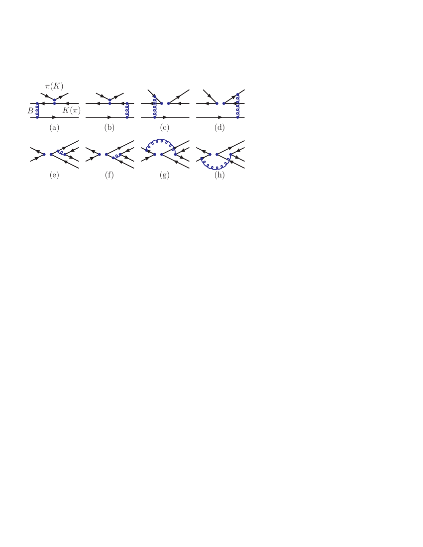
Figure 1: The Feynman diagrams for the LO contributions in the pQCD approach: (a,b) factorizable emission diagrams; (c,d) hard-spectator diagrams; (e-h) annihilation diagrams.

In the pQCD factorization approach, the leading order contributions to $B\to K\pi$ decays come from the eight Feynman diagrams as shown in Fig.1. Following Ref. ali2007 , we here also use the terms $(F_{e}^{LL},F_{e}^{LR},F_{e}^{SP})$ and $(M_{e}^{LL},M_{e}^{LR},M_{e}^{SP})$ to describe the contributions from the factorizable emission diagrams (Fig.1(a) and 1(b)) and non-factorizable emission diagrams (Fig.1(c) and 1(d)) through the $(V-A)(V-A)$, $(V-A)(V+A)$ and $(S-P)(S+P)$ operators, respectively. In a similar way, we also adopt $(F_{a}^{LL},F_{a}^{LR},F_{a}^{SP})$ and $(M_{a}^{LL},M_{a}^{LR},M_{a}^{SP})$ to stand for the contributions from the factorizable annihilation diagrams (Fig.1(e) and 1(f)) and non-factorizable annihilation diagrams (Fig.1(g) and 1(h)). From the analytic calculations we obtain all relevant decay amplitudes for the four $B\to K\pi$ decays:

By evaluating the emission diagrams Fig.1(a)-1(d), for example, we find the following decay amplitudes

$$F_{e}^{LL} = -F_{e}^{LR}=16\pi C_{F}M_{B}^{2}\int_{0}^{1}dx_{1}dx_{3}\,\int_{0}^{\infty}b_{1}db_{1}b_{3}db_{3}\;\phi_{B}(x_{1})$$ (5)

$$\times\left\{\left[(x_{3}+1)\phi_{3}^{A}(x_{3})+r_{3}(1-2x_{3})\left(\phi_{3}^{P}(x_{3})+\phi_{3}^{T}(x_{3})\right)\right]\cdot h_{a}(x_{1},x_{3},b_{1},b_{3})\;E_{e}(t_{a})\right.$$

$$\left.+2r_{3}\phi_{3}^{P}(x_{3})\cdot h_{b}(x_{1},x_{3},b_{1},b_{3})\;E_{e}(t_{b})\right\},$$

$$F_{e}^{SP} = 32\pi C_{F}M_{B}^{2}\int_{0}^{1}dx_{1}dx_{3}\,\int_{0}^{\infty}b_{1}db_{1}b_{3}db_{3}\;\phi_{B}(x_{1})r_{2}$$ (6)

$$\times\left\{\left[r_{3}(2+x_{3})\phi_{3}^{P}(x_{3})-r_{3}x_{3}\phi_{3}^{T}(x_{3})+\phi_{3}^{A}(x_{3})\right]\cdot h_{a}(x_{1},x_{3},b_{1},b_{3})\cdot E_{e}(t_{a})\right.$$

$$\left.+2r_{3}\phi_{3}^{P}(x_{3})\cdot h_{b}(x_{1},x_{3},b_{1},b_{3})\cdot E_{e}(t_{b})\right\},$$

$$M_{e}^{LL} = \frac{64}{\sqrt{6}}\pi C_{F}M_{B}^{2}\int_{0}^{1}dx_{1}dx_{2}dx_{3}\,\int_{0}^{\infty}b_{1}db_{1}b_{2}db_{2}\,\phi_{B}(x_{1})\phi_{2}^{A}(x_{2})$$ (7)

$$\times\left\{\left[\bar{x}_{2}\phi_{3}^{A}(x_{3})-x_{3}r_{3}\left(\phi_{3}^{P}(x_{3})-\phi_{3}^{T}(x_{3})\right)\right]\cdot h_{c}(x_{i},b_{1},b_{2})\;E_{e}^{{}^{\prime}}(t_{c})\right.$$

$$\left.+\left[(-x_{2}-x_{3})\phi_{3}^{A}(x_{3})+x_{3}r_{2}\left(\phi_{3}^{P}(x_{3})+\phi_{3}^{T}(x_{3})\right)\right]\cdot h_{d}(x_{i},b_{1},b_{2})\;E_{e}^{{}^{\prime}}(t_{d})\right\},$$

$$M_{e}^{LR} = \frac{64}{\sqrt{6}}\pi C_{F}M_{B}^{2}\int_{0}^{1}dx_{1}dx_{2}dx_{3}\,\int_{0}^{\infty}b_{1}db_{1}b_{2}db_{2}\,\phi_{B}(x_{1})$$ (8)

$$\times\left\{\left[\bar{x}_{2}\left(\phi_{2}^{P}(x_{2})+\phi_{2}^{T}(x_{2})\right)\phi_{3}^{A}(x_{3})+x_{3}r_{3}\left(\phi_{3}^{P}(x_{3})+\phi_{3}^{T}(x_{3})\right)\left(\phi_{2}^{P}(x_{2})-\phi_{2}^{T}(x_{2})\right)\right.\right.$$

$$\left.\left.+\bar{x}_{2}r_{3}\left(\phi_{3}^{P}(x_{3})-\phi_{3}^{T}(x_{3})\right)\left(\phi_{2}^{P}(x_{2})+\phi_{2}^{T}(x_{2})\right)\right]\cdot h_{c}(x_{i},b_{1},b_{2})\;E_{e}^{{}^{\prime}}(t_{c})\right.$$

$$\left.-\left[x_{2}\left(\phi_{2}^{P}(x_{2})-\phi_{2}^{T}(x_{2})\right)\phi_{3}^{A}(x_{3})+x_{2}r_{3}\left(\phi_{3}^{P}(x_{3})+\phi_{3}^{T}(x_{3})\right)\left(\phi_{2}^{P}(x_{2})-\phi_{2}^{T}(x_{2})\right)\right.\right.$$

$$\left.\left.+x_{3}r_{3}\left(\phi_{3}^{P}(x_{3})+\phi_{3}^{T}(x_{3})\right)\left(\phi_{2}^{P}(x_{2})+\phi_{2}^{T}(x_{2})\right)\right]\cdot h_{d}(x_{i},b_{1},b_{2})\;E_{e}^{{}^{\prime}}(t_{d})\right\},$$

$$M_{e}^{SP} = \frac{64}{\sqrt{6}}\pi C_{F}M_{B}^{2}\int_{0}^{1}dx_{1}dx_{2}dx_{3}\,\int_{0}^{\infty}b_{1}db_{1}b_{2}db_{2}\,\phi_{B}(x_{1})\phi_{2}^{A}(x_{2})$$ (9)

$$\times\left\{\left[(x_{2}-x_{3}-1)\phi_{3}^{A}(x_{3})+x_{3}r_{3}\left(\phi_{3}^{P}(x_{3})+\phi_{3}^{T}(x_{3})\right)\right]\cdot h_{c}(x_{i},b_{1},b_{2})\;E_{e}^{{}^{\prime}}(t_{c})\right.$$

$$\left.+\left[x_{2}\phi_{3}^{A}(x_{3})-x_{3}r_{3}\left(\phi_{3}^{P}(x_{3})-\phi_{3}^{T}(x_{3})\right)\right]\cdot h_{d}(x_{i},b_{1},b_{2})\;E_{e}^{{}^{\prime}}(t_{d})\right\},$$

where $r_{2}=m_{2}/m_{B}$, $r_{3}=m_{3}/m_{B}$ and $C_{F}=4/3$ is a color factor. The explicit expressions for the convolution functions $E_{e}(t_{a,})$ and $E_{a}^{{}^{\prime}}(t_{c,d})$, the hard scales $t_{a,b,c,d}$, and the hard functions $h_{a,b,c,d}(x_{i},b_{i})$ can be found in Ref. xiao2008a . By evaluating the annihilation diagrams Fig.1(e)-1(h) we can find the corresponding decay amplitudes $F_{a}^{LL,LR,SP}$ and $M_{a}^{LL,LR,SP}$, similar with those as given in Eqs.(34-38) in Ref. fan2013 .

Taking into account the contributions from different Feynman diagrams, the total decay amplitudes for $B^{0}\to K^{+}\pi^{-}$ and $B^{+}\to K^{+}\pi^{0}$ decays can be written explicitly as:

$${\cal A}(B^{0}\to K^{+}\pi^{-}) = V_{ub}^{*}V_{us}\;\left[f_{K}\;a_{1}F_{e}^{LL}+C_{1}\;M_{e}^{LL}\right]$$ (10)

$$-V_{tb}^{*}V_{ts}\Bigl{\{}f_{K}\left(a_{4}+a_{10}\right)F_{e}^{LL}+f_{K}(a_{6}+a_{8})\;F_{e}^{SP}+(C_{3}+C_{9})M_{e}^{LL}$$

$$+(C_{5}+C_{7})M_{e}^{LR}+f_{B}\left[\left(a_{4}-\frac{a_{10}}{2}\right)\;F_{a}^{LL}+\left(a_{6}-\frac{a_{8}}{2}\right)\;F_{a}^{SP}\right]$$

$$+\left(C_{3}-\frac{C_{9}}{2}\right)\;M_{a}^{LL}+\left(C_{5}-\frac{C_{7}}{2}\right)M_{a}^{LR}\Bigr{\}},\;$$

$$\sqrt{2}\;{\cal A}(B^{+}\to K^{+}\pi^{0}) = V_{ub}^{*}V_{us}\cdot\left\{\left[a_{1}f_{K}+a_{2}f_{\pi}\right]F_{e}^{LL}+(C_{1}+C_{2})M_{e}^{LL}+a_{1}f_{B}F_{a}^{LL}+C_{1}M_{a}^{LL}\right\}$$ (11)

$$-V_{tb}^{*}V_{ts}\cdot\Bigl{\{}\left(a_{4}+a_{10}\right)\left(f_{K}F_{e}^{LL}+f_{B}F_{a}^{LL}\right)+(a_{6}+a_{8})\left(f_{K}F_{e}^{SP}+f_{B}F_{a}^{SP}\right)$$

$$+(C_{3}+C_{9})\left(M_{e}^{LL}+M_{a}^{LL}\right)+(C_{5}+C_{7})\left(M_{e}^{LR}+M_{a}^{LR}\right)$$

$$+\frac{3}{2}(-a_{7}+a_{9})f_{\pi}\;F_{e}^{LL}+\frac{3}{2}C_{8}\;M_{e}^{SP}+\frac{3}{2}C_{10}\;M_{e}^{LL}\Bigr{\}},\;$$

where $a_{i}$ is the combination of the Wilson coefficients $C_{i}$ with the definitions: $a_{1,2}=C_{2,1}+\frac{C_{1,2}}{3}$, $a_{i}=C_{i}+\frac{C_{i+1}}{3}$ ( $a_{i}=C_{i}+\frac{C_{i-1}}{3}$) for $i=3,5,7,9$ ( $i=4,6,8,10$) respectively. The explicit expressions for $B^{0}\to K^{0}\pi^{0}$ and $B^{+}\to K^{0}\pi^{+}$ decays are similar with those as shown in Eqs.(10,11).

II.2 NLO contributions

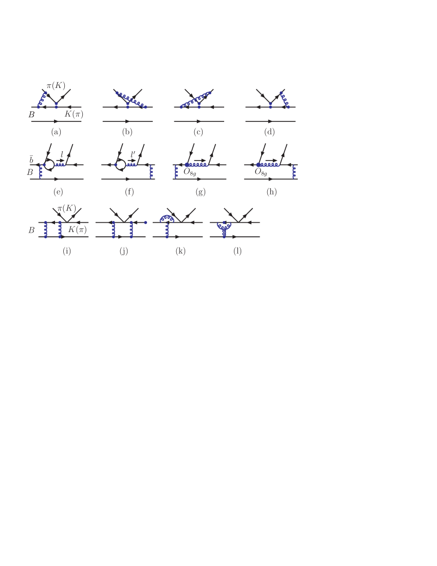
Figure 2: The typical Feynman diagrams for currently known NLO contributions: the vertex corrections (a-d); the quark-loop (e-f); the chromo-magnetic penguins (g-h); and the NLO contributions to form factors (i-l).

Based on the power counting rule in the pQCD factorization approach nlo05 , the following NLO contributions should be includednlo05 :

1. The Wilson coefficients $C_{i}(M_{W})$ at NLO level buras96 , the renormalization group evolution matrix $U(t,m,\alpha)$ at NLO level and the strong coupling constant $\alpha_{s}(t)$ at two-loop levelpdg2012 .

2. The currently known NLO contributions to hard kernel $H^{(1)}(\alpha_{s}^{2})$ include nlo05 ; o8g2003 ; prd85-074004 :

   • The vertex correction (VC)from the Feynman diagrams Fig.2(a)-2(d);

   • The NLO contributions from the quark-loops (QL) as shown in Fig.2(e)-2(f);

   • The NLO contributions from the operator $O_{8g}$ as shown in Fig.3(g)-3(h) o8g2003 ;

   • The NLO contributions to the form factors as shown in Fig.2(i)-2(l) prd85-074004 .

The still missing NLO parts in the pQCD approach are the $O(\alpha_{s}^{2})$ contributions from hard spectator diagrams and annihilation diagrams, as illustrated by Fig.5 in Ref. fan2013 . According to the general arguments as presented in Ref. nlo05 and explicit numerical comparisons of the contributions from different sources for $B\to K\pi$ decays as made in Ref. fan2013 one generally believe that these still missing NLO parts should be very small and can be neglected safely. The major reasons are the following:

1. For the non-factorizable spectator diagrams in Fig.1(c)-1(d), their LO contributions are strongly suppressed by the isospin symmetry and color-suppression with respect to the factorizable emission diagrams Fig.1(a)-1(b). The NLO contributions from Figs.5(a)-5(d) in Ref. fan2013 are higher order corrections to small LO quantities.

2. For the annihilation spectator diagrams at leading order, i.e. Figs.1(e)-1(h), they are power suppressed and generally much smaller with respect to the contributions from the emission diagrams Fig.1(a)-1(b). The NLO contributions from Figs.5(e)-5(h) in Ref. fan2013 are also the higher order corrections to the small LO quantities.

3. Taking $B^{+}\to K^{+}\eta$ decay as an example, as shown in Eq.(87) of Ref. fan2013 , the relative strength of the individual LO contribution ${\cal M}^{a+b}$ from the emission diagrams, ${\cal M}^{c+d}$ and ${\cal M}^{anni}$ from the spectator and the annihilation diagram respectively can be evaluated through the following ratio:

   $$|{\cal M}^{a+b}|^{2}:|{\cal M}^{c+d}|^{2}:|{\cal M}^{anni}|^{2}=3.23:0.02:0.33.$$ (12)

   One can see directly from the above ratio that the contribution from emission diagram is indeed dominant, while the contribution from ${\cal M}^{c+d}$ ( ${\cal M}^{anni}$ ) is less than $1\%$ ($10\%$) of the dominant one.

Based on about reasonable arguments and explicit numerical examinations, one can see that the still missing NLO parts in the pQCD approach are higher order corrections to those small LO quantities, and therefore should be very small and can be neglected safely. For more details of numerical comparisons, one can see Ref. fan2013 .

The vertex corrections from the Feynman diagrams as shown in Figs. 2(a)-2(d), have been calculated years ago in the QCD factorization appeoachbbns99 ; npb675 . Since there is no end-point singularity in the evaluations of Figs.2(a)-2(d), it is unnecessary to employ the $k_{T}$ factorization theorem here nlo05 . The NLO vertex corrections will be included by adding a same vertex function $V_{i}(M)$ to the corresponding Wilson coefficients $a_{i}(\mu)$ as in Refs. bbns99 ; npb675 ; xiao2008a .

For the $b\rightarrow s$ transition, the contributions from the various quark loops are given bynlo05

$$H_{eff}=-\sum_{q=u,c,t}\sum_{q^{{}^{\prime}}}\frac{G_{F}}{\sqrt{2}}V_{qb}V_{qs}^{*}\frac{\alpha_{s}(\mu)}{2\pi}C^{(q)}(\mu,l^{2})\left[\bar{s}\gamma_{\rho}\left(1-\gamma_{5}\right)T^{a}b\right]\left(\bar{q}^{{}^{\prime}}\gamma^{\rho}T^{a}q^{{}^{\prime}}\right),$$ (13)

where $l^{2}$ is the invariant mass of the gluon, which attaches the quark loops in Figs.2e and 2f. The expressions of the functions $C^{q}(\mu,l^{2})$ for $q=(u,c,t)$ can be found easily in Refs.nlo05 ; xiao2008a .

The magnetic penguin is another kind penguin correction induced by the insertion of the operator $O_{8g}$, as illustrated by Fig.2(g) and 2(h). The corresponding weak effective Hamiltonian contains the $b\to sg$ transition can be written as

$$H_{eff}^{mp}=-\frac{G_{F}}{\sqrt{2}}\frac{g_{s}}{8\pi^{2}}m_{b}\;V_{tb}V_{ts}^{*}\;C_{8g}^{eff}\left[\bar{s}_{i}\;\sigma^{\mu\nu}\;(1+\gamma_{5})\;T^{a}_{ij}\;G^{a}_{\mu\nu}\;b_{j}\right],$$ (14)

where $i,j$ are the color indices of quarks, $C_{8g}^{eff}=C_{8g}+C_{5}$ nlo05 is the effective Wilson coefficient.

For the sake of convenience we denote all current known NLO contributions except for those to the form factors by the term Set-A. For the four $B\to K\pi$ decays, the Set-A NLO contributions will be included in a simple way:

$${\cal A}_{\pi K} \to {\cal A}_{\pi K}+\sum_{q=u,c,t}\xi_{q}{\cal M}_{\pi K}^{(q)}+\xi_{t}{\cal M}_{\pi K}^{(g)},$$

$${\cal A}_{K\pi} \to {\cal A}_{K\pi}+\sum_{q=u,c,t}\xi^{\prime}_{q}{\cal M}_{K\pi}^{(q)}+\xi^{\prime}_{t}{\cal M}_{K\pi}^{(g)},$$ (15)

where $\xi_{q}=V_{qb}V_{qd}^{*}$, $\xi^{\prime}_{q}=V_{qb}V_{qs}^{*}$ with $q=u,c,t$, while the decay amplitudes ${\cal M}^{(q)}_{M_{i},M_{j}}$ and ${\cal M}^{(g)}_{M_{i},M_{j}}$ are of the form:

$${\cal M}^{(q)}_{\pi^{-}K^{+}} = -8m_{B}^{4}\frac{{C_{F}}^{2}}{\sqrt{2N_{c}}}\int_{0}^{1}dx_{1}dx_{2}dx_{3}\int_{0}^{\infty}b_{1}db_{1}b_{3}db_{3}\,\phi_{B}(x_{1})\left\{\left[(1+x_{3})\phi_{\pi}^{A}(x_{3})\phi_{K}^{A}(x_{2})\right.\right.$$ (16)

$$\left.\left.+2r_{\pi}\phi_{K}^{P}(x_{2})\phi_{\pi}^{A}(x_{3})+r_{\pi}(1-2x_{3})\phi_{K}^{A}(x_{2})(\phi_{\pi}^{P}(x_{3})+\phi_{\pi}^{T}(x_{3}))\right.\right.$$

$$\left.\left.+2r_{\pi}r_{K}\phi_{K}^{P}(x_{2})((2+x_{3})\phi_{\pi}^{P}(x_{3})-x_{3}\phi_{\pi}^{T}(x_{3}))\right]\right.$$

$$\left.\cdot\alpha_{s}^{2}(t_{a})h_{e}(x_{1},x_{3},b_{1},b_{3})\exp[-S_{ab}(t_{a})]C^{(q)}(t_{a},l^{2})\right.$$

$$\left.+\left[2r_{\pi}\phi_{K}^{A}(x_{2})\phi_{\pi}^{P}(x_{3})+4r_{\pi}r_{K}\phi_{K}^{P}(x_{2})\phi_{\pi}^{P}(x_{3})\right]\right.$$

$$\left.\cdot\alpha_{s}^{2}(t_{b})h_{e}(x_{3},x_{1},b_{3},b_{1})\exp[-S_{ab}(t_{b})]C^{(q)}(t_{b},l^{\prime 2})\right\},$$

$${\cal M}^{(g)}_{\pi^{-}K^{+}} = -16m_{B}^{6}\frac{{C_{F}}^{2}}{\sqrt{2N_{c}}}\int_{0}^{1}dx_{1}dx_{2}dx_{3}\int_{0}^{\infty}b_{1}db_{1}b_{2}db_{2}b_{3}db_{3}\,\phi_{B}(x_{1})$$ (17)

$$\cdot\left\{\left[(1-x_{3})\left[2\phi_{\pi}^{A}(x_{3})+r_{\pi}(3\phi_{\pi}^{P}(x_{3})+\phi_{\pi}^{T}(x_{3}))\right.\right.\right.$$

$$\left.\left.\left.+r_{\pi}x_{3}(\phi_{\pi}^{P}(x_{3})-\phi_{\pi}^{T}(x_{3}))\right]\phi_{K}^{A}(x_{2})\right.\right.$$

$$\left.\left.-r_{K}x_{2}(1+x_{3})(3\phi_{K}^{P}(x_{2})-\phi_{K}^{T}(x_{2}))\phi_{\pi}^{A}(x_{3})\right.\right.$$

$$\left.\left.-r_{\pi}r_{K}(1-x_{3})(3\phi_{K}^{P}(x_{2})+\phi_{K}^{T}(x_{2}))(\phi_{\pi}^{P}(x_{3})-\phi_{\pi}^{T}(x_{3}))\right.\right.$$

$$\left.\left.-r_{\pi}r_{K}x_{2}(1-2x_{3})(3\phi_{K}^{P}(x_{2})-\phi_{K}^{T}(x_{2}))(\phi_{\pi}^{P}(x_{3})+\phi_{\pi}^{T}(x_{3}))\right]\right.$$

$$\left.\cdot\alpha_{s}^{2}(t_{a})h_{g}(x_{i},b_{i})\exp[-S_{cd}(t_{a})]C_{8g}^{eff}(t_{a})\right.$$

$$\left.+\left[4r_{\pi}\phi_{K}^{A}(x_{2})\phi_{\pi}^{P}(x_{3})+2r_{K}r_{\pi}x_{2}(3\phi_{K}^{P}(x_{2})-\phi_{K}^{T}(x_{2}))\phi_{\pi}^{P}(x_{3})\right]\right.$$

$$\left.\alpha_{s}^{2}(t_{b})h^{\prime}_{g}(x_{i},b_{i})\exp[-S_{cd}(t_{b})]C_{8g}^{eff}(t_{b})\right\},$$

$$\sqrt{2}{\cal M}^{(q)}_{K^{0}\pi^{0}} = {\cal M}^{(q)}_{\pi^{-}K^{+}}={\cal M}^{(q)}_{K^{0}\pi^{+}}={\cal M}^{(q)}_{K^{+}\pi^{0}},$$ (18)

$$\sqrt{2}{\cal M}^{(g)}_{K^{0}\pi^{0}} = {\cal M}^{(g)}_{\pi^{-}K^{+}}={\cal M}^{(g)}_{K^{0}\pi^{+}}={\cal M}^{(g)}_{K^{+}\pi^{0}},$$ (19)

where the expressions of the Sudakov factors $S_{ab}(t_{i})$ and $S_{cd}(t_{i})$, the functions $C^{(q)}(t_{a},l^{2})$ and $C^{(q)}(t_{b},l^{\prime 2})$, can be found easily in Refs. nlo05 ; xiao2008a .

In Ref. prd85-074004 , the authors derived the $k_{\rm T}$-dependent NLO hard kernel $H^{(1)}$ for the $B\to\pi$ transition form factor. Here we quote their results directly, and extend the expressions to the $B\to K$ transitions under the assumption of $SU(3)$ flavor symmetry. At the NLO level, the hard kernel function $H$ can then be written as

$$H=H^{(0)}(\alpha_{s})+H^{(1)}(\alpha_{s}^{2})=\left[1+F(x_{1},x_{3},\mu,\mu_{f},\eta,\zeta_{1})\right]H^{(0)}(\alpha_{s}),$$ (20)

where the expression of the NLO factor $F(x_{1},x_{3},\mu,\mu_{f},\eta,\zeta_{1})$ can be found in Eq. (56) of Ref. prd85-074004 .

III Numerical Results and Discussions

In numerical calculations, the following input parameters will be usedpdg2012 ( all the masses, QCD scale and decay constants are in units of $GeV$):

$$\Lambda_{QCD} = 0.25\;,\quad m_{W}=80.40\;,\quad m_{B}=5.28\;,\quad m_{\pi}=0.14,\quad m_{K}=0.494\;;$$

$$f_{\pi} = 0.13,\quad f_{K}=0.16,\quad\tau_{B^{0}}=1.528\;ps,\quad\tau_{B^{+}}=1.643\;ps.$$ (21)

For the CKM matrix elements in the Wolfenstein parametrization, we use $\lambda=0.2254$, $A=0.817$, $\bar{\rho}=0.136^{+0.019}_{-0.018}$ and $\bar{\eta}=0.348\pm 0.013$ pdg2012 . For the Gegenbauer moments and other relevant input parameters, we use ball2006

$$a_{1}^{\pi} = 0,\quad a_{1}^{K}=0.06,\quad a_{2}^{\pi}=a_{2}^{K}=0.25\pm 0.15,\quad a_{4}^{\pi}=-0.015,\quad a_{4}^{K}=0,$$

$$\rho_{\pi} = m_{\pi}/m_{0}^{\pi},\quad\rho_{K}=m_{K}/m_{0}^{K},\quad\eta_{3}=0.015,\quad\omega_{3}=-3.0,$$ (22)

with the chiral mass $m_{0}^{\pi}=1.4\pm 0.1$ GeV, and $m_{0}^{K}=1.6\pm 0.1$ GeV.

From the decay amplitudes and the input parameters, it is straightforward to calculate the branching ratios and CP violating asymmetries for the four considered $B\to K\pi$ decays nlo05 ; xiao2008a .

In Table I and II, we show the LO and NLO pQCD predictions for the branching ratios and the direct CP violating asymmetries of the considered four $B\to K\pi$ decays. In Table I and II, we list only the central values of the LO pQCD predictions in column two, and the central values and the major theoretical errors simultaneously in column four. The first error arises from the uncertainty of $\omega_{B}=0.40\pm 0.04$ GeV, the second one from the uncertainty of $a_{2}^{\pi,K}=0.25\pm 0.15$, and the third one is induced by the variations of both $m_{0}^{K}=1.6\pm 0.1$ GeV and $m_{0}^{\pi}=1.4\pm 0.1$ GeV. The errors induced by the uncertainties of other input parameters are very small and have been neglected. As a comparison, we also show the partial pQCD predictions obtained in this work ( labeled by Set-A in column three ) and those as given in Ref. nlo05 in the column five, where the same Set-A NLO contributions are included. One can see from those numerical results that:

1. For branching ratios, the central values of pQCD predictions as given in column three in Table I are smaller than those as shown in column five by about thirty percent, such difference are largely induced by the change of the lower cutoff of the hard scale $t$ from $\mu_{0}=0.5$ GeV in Ref. nlo05 to $\mu_{0}=1$ GeV here, because it may be conceptually incorrect to evaluate the Wilson coefficients at scales down to 0.5 GeV xiao2008a ; beneke07 . For direct CP violating asymmetries, as shown in the third and fifth column of Table II, the changes of the pQCD predictions due to the variation of $\mu_{0}$ are rather small, this is consistent with the general expectation.

2. Analogous to the case for $B\to K\eta^{(\prime)}$ decays as shown explicitly in Table VIII and IX in Ref. fan2013 , the NLO contributions to the decay amplitudes from the vertex, the quark-loop and the magnetic penguins are largely canceled from each other, and in turn leaving only a roughly $10\%$ enhancement to the LO pQCD predictions of the branching ratios.

3. As listed in Table I of Ref. wang2012 , the NLO contribution to the form factor for $B\to\pi$ ($B\to K$) transition can provide a $18\%$ ($15\%$) enhancement to the corresponding LO result:

   $$F_{0}^{LO}(0)(B\to\pi) = 0.22\pm 0.04\longrightarrow F_{0}^{NLO}(0)(B\to\pi)=0.26\pm 0.04,$$

   $$F_{0}^{LO}(0)(B\to K) = 0.27\pm 0.05\longrightarrow F_{0}^{NLO}(0)(B\to K)=0.31\pm 0.05.$$ (23)

   Such enhancement to form factors $F_{0}^{B\to\pi}(0)$ and $F_{0}^{B\to K}(0)$ can in turn result in an additional $12\%$ to $18\%$ enhancement to branching ratios relative to the results in the third column with the label ”Set-A”, as illustrated clearly by the numerical results in column four of Table I, and consequently lead to a very good agreement between the NLO pQCD predictions and the measured values within errors.

4. For ${\cal A}_{CP}^{dir}(B^{0}\to K^{0}\pi^{0})$ and ${\cal A}_{CP}^{dir}(B^{+}\to K^{0}\pi^{+})$, the pQCD predictions agree well with the data.

5. At the leading order, the pQCD predictions for ${\cal A}_{CP}^{dir}(B^{0}\to K^{+}\pi^{-})$ and ${\cal A}_{CP}^{dir}(B^{+}\to K^{+}\pi^{0})$ are indeed similar in both the sign and the magnitude, $-12.6\%$ vs $-8.6\%$, as generally expected. After the inclusion of the NLO contributions, however, they become rather different as can be seen from Table II. The NLO pQCD predictions, consequently, become agree well with the data. One can also see that the pQCD predictions for ${\cal A}_{CP}^{dir}(B^{0}\to K^{+}\pi^{-})$ and ${\cal A}_{CP}^{dir}(B^{+}\to K^{+}\pi^{0})$ remain basically unchanged when the NLO corrections to the form factors are taken into account.

Table 1: The LO and NLO pQCD predictions for branching ratios $Br(B\to K\pi)$ (in units of $10^{-6}$ ), the previous pQCD predictions in Ref. nlo05 and the relevant data pdg2012 ; hfag2012 also be listed in last two columns.

Decay modes	LO	Set-A	NLO: This Work	pQCDnlo05	Data
$B^{0}\rightarrow K^{0}\pi^{0}$	$6.3$	$6.6$	$7.4^{+2.2+1.3+0.9}_{-1.5-1.2-0.9}$	$9.1^{+5.6}_{-3.3}$	$9.9\pm 0.5$
$B^{0}\rightarrow K^{+}\pi^{-}$	$14.4$	$15.3$	$17.7^{+5.5+2.6+2.0}_{-3.8-2.4-2.0}$	$20.9^{+15.6}_{-6.3}$	$19.6\pm 0.5$
$B^{+}\rightarrow K^{+}\pi^{0}$	$10.1$	$10.6$	$12.5^{+4.0+1.7+1.3}_{-2.8-1.6-1.2}$	$13.9^{+10}_{-5.6}$	$12.9\pm 0.5$
$B^{+}\rightarrow K^{0}\pi^{+}$	$17.5$	$18.4$	$21.5^{+6.7+3.4+2.8}_{-4.7-3.1-2.3}$	$24.5^{+13.6}_{-8.1}$	$23.8\pm 0.7$

Table 2: The same as in Table I, but for the pQCD predictions for the direct CP violations ${\cal A}_{CP}^{dir}(B\to K\pi)$ (in units of $10^{-2}$).

Decay modes	LO	Set-A	NLO: This Work	pQCDnlo05	Data
${\cal A}_{CP}^{dir}(B^{0}\to K^{0}\pi^{0})$	$-2.2$	$-7.0$	$-7.9^{+0.3+0.8+0.4}_{-0.23-0.9-0.5}$	$-7\pm 3$	$0\pm 13$
${\cal A}_{CP}^{dir}(B^{+}\to K^{0}\pi^{+})$	$-0.75$	$0.40$	$0.38^{+0.09+0.02+0.03}_{-0.11-0.07-0.05}$	$0\pm 0$	$-1.5\pm 1.2$
${\cal A}_{CP}^{dir}(B^{0}\to K^{+}\pi^{-})$	$-12.6$	$-6.4$	$-6.5^{+2.1}_{-2.0}\pm 2.3\pm 0.3$	$-9^{+6}_{-8}$	$-8.7\pm 0.8$
${\cal A}_{CP}^{dir}(B^{+}\to K^{+}\pi^{0})$	$-8.6$	$2.0$	$2.2^{+1.7}_{-1.8}\pm 1.2\pm 0.1$	$-1^{+3}_{-5}$	$3.7\pm 2.1$

In summary, we studied the $B\to K\pi$ decays by employing the pQCD factorization approach. We focus on checking the effects of all currently known NLO contributions to the branching ratios and direct CP violations of the considered decay modes, especially the rule of the NLO corrections to the form factors $F_{0}^{B\to\pi}(q^{2})$ and $F_{0}^{B\to K}(q^{2})$. Based on the numerical calculations and the phenomenological analysis, the following points have been observed:

1. Besides the $10\%$ enhancement from the Set-A NLO contributions, the NLO contributions to the form factors can provide an additional $\sim 15\%$ enhancement to the branching ratios, and lead to a very good agreement with the data.

2. With the inclusion of all known NLO contributions, the NLO pQCD predictions are

   $${\cal A}_{CP}^{dir}(B^{0}\to K^{+}\pi^{-})=(-6.5\pm 3.1)\%,\quad{\cal A}_{CP}^{dir}(B^{+}\to K^{+}\pi^{0})=(2.2\pm 2.0)\%,$$ (24)

   where the theoretical errors have been added in quadrature, which agree well with the data.

References

• (1) J.ย Beringer et al. (Particle Data Group), Phys. Rev. D 86, 010001 (2012).
• (2) Y.ย Amhis et al., (Heavy Flavor Averaging Group), arXiv:1207.1158 [hep-ex].
• (3) R.ย Aaij et al. (LHCb Collaboration), Phys. Rev. Lett. 108, 201601 (2012).
• (4) H.N.ย Li, S.ย Mishima, A.I.ย Sanda, Phys. Rev. D 72, 114005 (2005).
• (5) H.N.ย Li, Y.L.ย Shen, and Y.M.ย Wang, Phys. Rev. D 85, 074004 (2012).
• (6) H.N.ย Li, Prog. Part. $\&$ Nucl. Phys. 51, 85 (2003), and reference therein.
• (7) Y.Y.ย Keum, H.N.ย Li and A.I.ย Sanda, Phys. Lett. B 504, 6 (2001); Y.Y.ย Keum, H.N.ย Li and A.I.ย Sanda, Phys. Rev. D 63, 054008 (2001).
• (8) C.D.ย Lรผ, K.ย Ukai and M.Z.ย Yang, Phys. Rev. D 63, 074009 (2001).
• (9) Z.J.ย Xiao, Z.Q.ย Zhang, X.ย Liu, and L.B.ย Guo, Phys. Rev. D 78, 114001 (2008).
• (10) P.ย Ball, J. High Energy Phys. 9809, 005 (1998); J. High Energy Phys. 9901, 010 (1999); P.ย Ball and R. Zwicky, Phys. Rev. D 71, 014015 (2005); P.ย Ball, V.M.ย Braun, and A.ย Lenz, J. High Energy Phys. 0605 (2006) 004.
• (11) Y.ย Li, C.D.ย Lรผ, Z.J.ย Xiao, and X.Q.ย Yu, Phys. Rev. D 70, 034009 (2004).
• (12) A.ย Ali, G.ย Kramer, Y.ย Li, C.D.ย Lรผ, Y.L.ย Shen, W.ย Wang, and Y.M.ย Wang, Phys. Rev. D 76, 074018 (2007);
• (13) Y.Y.ย Fan, W.F.ย Wang, S.ย Cheng, and Z.J.ย Xiao, Phys. Rev. D 87, 094003 (2013).
• (14) G.ย Buchalla, A.J.ย Buras, and M.E.ย Lautenbacher, Rev. Mod. Phys. 68, 1215 (1996)
• (15) S.ย Mishima and A.I.ย Sanda, Prog. Theor. Phys. 110, 549 (2003).
• (16) M.ย Beneke, G.ย Buchalla, M.ย Neubert and C.T.ย Sachrajda, Phys. Rev. Lett. 83, 1914 (1999); Nucl. Phys. B 591, 313 (2000).
• (17) M.ย Beneke and M.ย Neubert, Nucl. Phys. B 675, 333 (2003).
• (18) M.ย Beneke, Nucl. Phys. B, Proc. Suppl. 170, 57 (2007).
• (19) W.F. Wang and Z.J. Xiao, Phys. Rev. D , 86, 114025 (2012).