Lognormal intensity distribution of the FUV continuum background shortward of Ly$\alpha$

Abstract

The diffuse far-ultraviolet (FUV) continuum radiation “longward” of Ly$\alpha$ (1216Å) is well known to correlate with the dust emission at 100 $\mu$m. However, it has been claimed that the FUV continuum background “shortward” of Ly$\alpha$ shows very weak or no correlation with the 100 $\mu$m emission. In this paper, the observational data of the diffuse FUV radiation by the Far Ultraviolet Spectroscopic Explorer is reexamined in order to investigate the correlation between the diffuse FUV radiation shortward of Ly$\alpha$ and the 100 $\mu$m emission. Large fluctuations were confirmed in the linear-linear correlation plots, but good correlations were found in the log-log plots. The large fluctuations in the linear-linear plots, and thus poor correlations, between the FUV and 100 $\mu$m intensities were attributed to the lognormal property of the FUV intensity distribution. The standard deviation of the intensity distribution of the FUV radiation shortward of Ly$\alpha$ was found to be $\sigma_{\log I}=0.16-0.25$. The result is consistent with that obtained not only for the FUV radiation longward of 1216Å, but also with the dust column density measurements of various molecular clouds. This implies that most of the diffuse FUV radiation shortward of Ly$\alpha$ is dust-scattered light in the turbulent interstellar medium. The diffuse FUV data obtained from the Voyager missions was also investigated. However, much wider random fluctuations were found compared with the FUSE data, which is most likely due to the systematic difficulties in data reduction of the Voyager data.

1. Introduction

The far-ultraviolet (FUV) continuum background in the wavelength longer than Ly$\alpha$ (1216Å; hereafter, FUV-L) has been investigated extensively and found to correlate with the 100 $\mu$m emission and neutral hydrogen (H I) column density, and thus to be mostly starlight scattered by interstellar dust (Paresce et al., 1980; Bowyer, 1991; Witt et al., 1997; Schiminovich et al., 2001; Murthy et al., 2010; Seon et al., 2011a, b). Since gas and dust are well mixed in the interstellar medium (ISM) (e.g., Boulanger & Pérault, 1988; Cox & Mezger, 1989) and the intensity of the scattered light is roughly proportional to the dust column density in the optically thin limit, the diffuse scattered light should exhibit a signature of the ISM density structure. The probability distribution functions (PDFs) of the three-dimensional densities and column densities of the turbulent ISM are well known to be close to lognormal not only through numerical simulations (Vázquez-Semadeni, 1994; Nordlund & Padoan, 1999; Klessen, 2000; Ostriker et al., 2001; Wada & Norman, 2001; Burkhart & Lazarian, 2012) but also through observations (Lada et al., 1994; Berkhuijsen & Fletcher, 2008; Hill et al., 2008; Seon, 2009; Padoan et al., 1997; Lombardi et al., 2006, 2008; Kainulainen et al., 2009; Froebrich & Rowles, 2010; Schneider et al., 2013). Recently, Seon et al. (2011a) found evidence that the PDF of the FUV-L continuum background intensity is lognormal, and this is attributable to the turbulent nature of the ISM.

Observations of the diffuse continuum background at the FUV wavelength band shortward of Ly$\alpha$ (hereafter, FUV-S) have been relatively scarce. The earliest observations of the FUV-S background were those of Belyaev et al. (1971) from Venera 5 and 6. Further photometric observations obtained the upper limits of the diffuse FUV-S continuum background (Henry, 1973; Paresce & Bowyer, 1976; Bixler et al., 1984; Opal & Weller, 1984). The most extensive observations of the FUV-S continuum background came from the ultraviolet spectrographs (UVSs) aboard the two Voyager spacecraft (Sandel et al., 1979; Holberg, 1986; Murthy et al., 1991, 1999, 2012). The Voyager 1 and 2 UVSs observed the diffuse FUV background from 1977 to 2001 and 1998, respectively. The entire data set of the observations were published by Murthy et al. (2012). Murthy et al. (1999) did not find a correlation between the diffuse FUV-S background and the H I column density. It was also claimed that the FUV-S background correlates with the integrated stellar fluxes, which presumably trace the local radiation field in each line of sight. However, several difficulties in the Voyager data set and/or the analyses have been identified (Edelstein et al. 2000; see Section 3.2 for details), and these may prevent proper interpretation of the Voyager results. Murthy & Sahnow (2004) used serendipitous observations from the Far Ultraviolet Spectroscopic Explorer (FUSE) to probe the diffuse FUV-S background. Only a very weak correlation was found between the FUV-S flux and the dust 100 $\mu$m emission; however, it had large fluctuations and it was concluded that the FUV-S sky is very patchy with both dark and bright regions. These results were attributed to the differences in the local radiation field.

Meanwhile, it should be noted that even the FUV-L continuum and 100 $\mu$m intensities show large fluctuations in the linear-linear correlation plots due to the lognormality of their intensity PDFs (Seon et al., 2011a). Seon et al. (2011a) found that the correlation of the FUV-L continuum background with the local stellar radiation field was less significant than with the dust thermal emission at 100 $\mu$m. Therefore, it can be speculated that the weak or no correlation between the FUV-S continuum and 100 $\mu$m intensities is related to the lognormal properties of the FUV-S intensity PDF. This was a key motivation to reexamine the FUV-S background data observed with the FUSE mission (Murthy & Sahnow, 2004) in order to determine whether the large fluctuations of the FUV-S background data could be explained using the lognormal density PDF of the ISM. The data obtained from the Voyager (Murthy et al., 2012) missions was also reexamined for completeness. In Section 2, the correlation properties between two lognormal random variables are investigated. The diffuse FUV-S continuum data are analyzed in Section 3. Finally, concluding remarks are given in Section 4.

2. Correlation between Two Lognormal Variables

As will be seen in Section 3, when the correlation between the FUV-S and 100 $\mu$m intensities is examined in a linear-linear plot, a higher variance of the FUV-S intensity is found as the 100 $\mu$m intensity increases, and vice versa. This tendency can be understood if the PDFs of the two random variables, which are linearly dependent on each other, are lognormal. A lognormal PDF for variable $I$ is defined as follows:

$$P(\ln I)d\ln I=\frac{1}{\sqrt{2\pi}\sigma_{\ln I}}\exp\left[-\frac{\left(\ln I-\left\langle\ln I\right\rangle\right)^{2}}{2\sigma_{\ln I}^{2}}\right]d\ln I.$$ (1)

Here, the mean value $\left\langle\ln I\right\rangle$ of the logarithmic quantity $\ln I$ is related to the linear mean value $\left\langle I\right\rangle$ by $\left\langle I\right\rangle=\left\langle\ln I\right\rangle e^{(1/2)\sigma_{\ln I}^{2}}$. The variance ($\sigma_{\ln I}^{2}$) of $\ln I$ is related to the variance ($\sigma_{I}^{2}$) or “relative” variance ($\sigma_{I/\left\langle I\right\rangle}^{2}=\sigma_{I}^{2}/\left\langle I\right\rangle^{2}$) of $I$ by $\sigma_{I/\left\langle I\right\rangle}^{2}=\exp\left(\sigma_{\ln I}^{2}\right)-1$ or $\sigma_{\ln I}^{2}=\ln(\sigma_{I/\left\langle I\right\rangle}^{2}+1)$. Therefore, a constant variance of $\ln I$ ($\sigma_{\ln I}^{2}=$ constant) yields a constant relative variance ($\sigma_{I/\left\langle I\right\rangle}^{2}=$ constant) of $I$, and thus a linearly increasing standard deviation of $I$ with mean value $\left\langle I\right\rangle$, i.e. $\sigma_{I}\propto\left\langle I\right\rangle$.

This property causes a rapidly increasing fluctuation with intensity in a linear-linear correlation plot between two lognormal variables. If two random variables (i.e. $x$ and $y$) are linearly correlated on average, i.e.

$$\left\langle y\right\rangle=a\left\langle x\right\rangle+b,$$ (2)

and their PDFs are lognormal, the correlation plot between them would exhibit large variances. Figure 1 demonstrates correlation between two lognormal variables in which the two variables $x$ and $y$ were assumed to be related by the linear equation $\left\langle y\right\rangle=70\left\langle x\right\rangle+2500$, as denoted by the red curves. The mean value $\left\langle x\right\rangle$ varied from 1.5 to 6400 in steps of 0.018 dex, and the two quantities ($x$ and $y$) were randomly generated to have lognormal distributions with standard deviations of $\sigma_{\log x}=\sigma_{\log y}=0.2$. Figures 1(a) and 1(b) present the correlation plots between $x$ and $y$, and between $\log x$ and $\log y$, respectively. It is evident that the correlation plot between the linear quantities shows no clear correlation, but rather large fluctuations for a given range of $x$, while the plot between the logarithmic quantities shows a clear correlation.

Therefore, the correlation between two lognormal quantities should be examined with logarithmic values. In the log-log plot, the linear relationship between the two logarithmic quantities may then be obtained by fitting the two quantities to the following equation:

$$\left\langle\log y\right\rangle=\log\left(a10^{\log x}+b\right),$$ (3)

which is equivalent to Equation (2). The standard deviation or variance of $\log y$ can also be derived by fitting the PDF of $\Delta\log y\equiv\log y-\left\langle\log y\right\rangle$ to a Gaussian function. Figures 1(c) and 1(d) present the $\Delta\log y$ versus $\log x$ and the PDF of $\Delta\log y$ plots, respectively. The red curve in Figure 1(d) is the Gaussian PDF for $\Delta\log y$ with a standard deviation of 0.2, which corresponds to the standard deviation of $\log y$. In this manner, it will be shown that the FUV-S continuum background is well described using a lognormal PDF and the standard deviation of the PDF is derived in the following section.

3. Data Analysis

3.1. FUSE data

The FUSE mission is described in detail by Moos et al. (2000). The present study used the FUSE S405/505 program data that was reduced by Murthy & Sahnow (2004), instead of reprocessing the raw data. The S405/505 program observed the blank sky regions near a number of alignment stars. Murthy & Sahnow (2004) integrated the FUV-S fluxes over six bands ($\lambda\lambda$987–1021, $\lambda\lambda$1035–1081, $\lambda\lambda$1100–1134, $\lambda\lambda$1134–1180, $\lambda\lambda$1175–1142, and $\lambda\lambda$1129–1195) that were selected to avoid airglow lines, and the diffuse astronomical signal data was tabulated as presented in their Table 2. The six bands are denoted as “F1” to “F6”, and the total intensity averaged over the six bands is “TOT”. In the present analysis, the Improved Reprocessing of the IRAS Survey (IRIS) map is used for the dust thermal emission at 100 $\mu$m (Miville-Deschênes & Lagache, 2005). The 100 $\mu$m map from Schlegel et al. (1998) was also used and no significant differences were found when compared with the results obtained with the IRIS map. The main difference between the IRIS map and the Schlegel et al. (1998) map is that the IRIS map was obtained by taking into account the variation of the detector gain with brightness at scales smaller than 1^∘ while a constant gain factor was assumed in the Schlegel et al. (1998) map.

First, the FUV-S intensities in the six bands are plotted against the 100 $\mu$m intensity in linear-linear plots in the first column of Figure 2. As noted by Murthy & Sahnow (2004), the linear-linear plots show very weak correlations and large fluctuations in the FUV-S intensity for a given range of the 100 $\mu$m intensity. The correlation relation between the $\log I_{{\rm FUV}}$ and $\log I_{{\rm IR}}$ is shown in the second column of Figure 2. It is clear that the large fluctuations seen in the linear-linear plots have largely disappeared, and the correlation between the FUV-S and 100 $\mu$m intensities is more distinct. The correlation between two quantities, e.g. the FUV-S intensity ($I_{{\rm FUV}}$) and the 100 $\mu$m intensity ($I_{{\rm IR}}$), is usually investigated using a linear equation between the two linear intensities, i.e. $\left\langle I_{{\rm FUV}}\right\rangle=a\left\langle I_{{\rm IR}}\right\rangle+b$. However, in this study, the correlation relations were fitted with Equation (3) and the resulting best-fit parameters are presented in the second column of Figure 2. The best-fit curves are also shown in red in the first and second columns. In the second column, the Pearson correlation coefficient ($\rho$), which is defined as the covariance of the two variables divided by the product of their standard deviations, is also denoted. The coefficient is normally sensitive to outliers and thus the strong correlations in Figure 2 could be suspected to be the results of the highest intensity data ($I_{100\mu{\rm m}}\sim 2.5\times 10^{3}$ MJy sr^-1). Ignoring the highest intensity data lowered the correlation coefficients, but no more than $\sim 0.1$. Therefore, the strong correlations between the FUV-S and 100 $\mu$m intensities are not due to the highest intensity data. The residuals $\Delta\log I_{{\rm FUV}}\equiv\log I_{{\rm FUV}}-\left\langle\log I_{{\rm FUV}}\right\rangle$, after subtracting the linear dependency of the FUV-S intensity on the 100 $\mu$m intensity, versus $\log I_{{\rm IR}}$ are shown in the third column in Figure 2. It is noted that the residuals $\Delta\log I_{{\rm FUV}}$ are more or less independent of $\log I_{{\rm IR}}$. However, if the residuals were drawn in linear scale, they would exhibit extended asymmetric tails to high intensity values. This property is a characteristic of the lognormal PDF.

In order to confirm that the fluctuations from the average linear dependence are represented by lognormal distributions, the histograms of the residuals $\Delta\log I_{{\rm FUV}}$ were fitted with a Gaussian function. In the fit, the Poisson error ($\sigma_{i}=\sqrt{N_{i}}$ in the bin $i$) was assumed, where $N_{i}$ is the number of data points in the bin. The results are shown in the last column of Figure 2. It is clear that the PDFs are well represented by the lognormal distributions, except some of the highest intensity bins. The standard deviations of the logarithmic FUV-S intensities $\sigma_{\log I}=0.16-0.25$ or $\sigma_{\ln I}=(\ln 10)\sigma_{\log I}=0.37-0.58$ were obtained from the residual distributions. The standard deviations in each wavelength band are also shown in the figure. Then, the relative standard deviations or contrasts of the FUV-S intensity are given by $\sigma_{I/\left\langle I\right\rangle}=0.38-0.63$.

Murthy et al. (1999) claimed that there is a strong correlation of the FUV-S intensity obtained using the $Voyager$ UVSs with the stellar flux from the OB stars, which presumably traces the local FUV radiation in each line of sight, while there is no correlation with tracers of the ISM. Hence, the correlation of the FUV-S intensity with the stellar flux at $\sim$1565 Å is examined using the TD-1 stellar catalog (Thompson et al., 1978), as done by Murthy et al. (1999). The TD-1 catalog presents the absolute UV fluxes in four wavelength bands (centered at 1565, 1965, 2365, and 2740 Å, each being 310–330 Å wide). The stellar fluxes within 2^∘ of the observed position were integrated in order to calculate the “stellar equivalent diffuse intensity (SEDI)” (Hurwitz et al., 1991; Seon et al., 2011a). Figure 3 presents the correlation plot between the FUV-S intensity and the TD-1 SEDI. The Pearson correlation coefficients are also denoted in the third and fourth columns. It is clear that there is no apparent correlation in the linear-linear plots, while the log-log plots reveal some correlations. It is also noted that the correlations with the stellar flux are weaker than those with the 100 $\mu$m intensity. A weaker correlation in the FUV-L intensity with the local stellar flux than that with the ISM tracers was also found (Seon et al., 2011a). These results do not support the previous claim that the diffuse FUV continuum background correlates strongly with the local stellar radiation field.

3.2. Voyager data

The most extensive observations of the FUV-S continuum background are provided by the two Voyager UVSs. The Voyager UVSs provide spectral data of the diffuse FUV radiation in the wavelength range of $\sim 540$–1700Å. Therefore, the same analyses were performed on the Voyager FUV-S data in the wavelength range of 987–1200Å (obtained from Murthy et al. 2012) as on the FUSE data. Figure 4 presents the linear-linear and log-log correlation plots, $\Delta\log I_{{\rm FUV}}$ versus $I_{100\mu{\rm m}}$, and the $\Delta\log I_{{\rm FUV}}$ histogram, as in Figure 2 for the FUSE data. The Pearson’s correlation coefficients are also shown with the log-log correlation plots. Unlike the FUSE data, the correlation between the Voyager data and the 100 $\mu$m emission is very weak not only in the linear-linear plots, but also in the log-log plots. The best-fit slopes ($a$) are less steep than those found for the FUSE data because the Voyager data were mostly obtained at sightlines with low 100 $\mu$m intensity. However, the PDFs of the residuals from the best-fit linear curves can still be represented using lognormal functions, but with much broader widths than those for the FUSE data. The best-fit curves in Figure 4(b) do not seem to follow the data at first glance. Robustness of the results was assessed by varying the initial parameter values for regression. Results were always the same regardless of the adopted initial values. The symmetrical histograms of the residuals in Figure 4(d) also indicate the robustness of the results.

Figure 5 shows the correlation between the FUV-S intensity and the local radiation field. It is noted that the correlation of the Voyager 1 data with the local radiation field is slightly better than that with the dust thermal emission, but not as strong as Murthy et al. (1999) claimed. However, the correlation of the Voyager 2 data with the local radiation field is slightly worse than that with the dust emission. Therefore, it is not plausible to discriminate using the Voyager data whether the correlation of the FUV-S intensity with the 100 $\mu$m intensity is better or not than that with the local radiation field.

The poor correlation between the Voyager FUV-S data and the 100 $\mu$m emission, and the large fluctuation of the FUV-S intensity even in the log-log plots may be attributable to unknown difficulties in the data reduction of the Voyager data (Edelstein et al., 2000). The measurement of the diffuse flux with the Voyager UVS data requires complex corrections for noise components that are much larger than the astronomical signal. There are three components in a typical Voyager spectrum: instrumental dark noises from the spacecraft’s radioisotope thermoelectric generator, four interplanetary emission lines and their associated broad scattering wings, and cosmic signals (which originate beyond the solar system). The most prominent emission line feature in the observed spectrum is the heliospheric Ly$\alpha$ at 1216Å, which is reflected by the calibration plate into the spectrometer. The Ly$\alpha$ feature is so intense that its scattering wings extend over almost the entire spectrum. Although Murthy et al. (1991, 1999, 2012) claim that the noise components are relatively well determined, Edelstein et al. (2000) note that there is still a significant danger of systematic effects, which have not been fully appreciated in the data reduction procedures of the Voyager data, which dominate the random effects.

In order to confirm the systematic effects in the Voyager data reduction, the Voyager FUV-L data obtained in the wavelength range of $\sim 1300$–1700Å was also analyzed. Because the FUV-L continuum intensity is well known to correlate with the 100 $\mu$m intensity, the Voyager FUV-L data should exhibit a good correlation with the 100 $\mu$m intensity if there is no serious problem in the data reduction of the Voyager data. The Pearson’s correlation coefficients between the FUV-L intensity and the 100$\mu$m intensity were $-0.06$ and 0.12 for the Voyager 1 and 2 data, respectively. These values are worse than that for the FUV-S data. Therefore, it is highly likely that the systematic effects yielded large random noises in the diffuse FUV-S fluxes of the Voyager and hampered the correlation analysis between the FUV-S background and the ISM tracers. Thus, the results obtained using the Voyager UVS spectrometers are not discussed further in this paper.

4. Concluding Remarks

It was found that the intensity distribution of the FUV-S continuum background obtained using the FUSE mission is well represented by a lognormal distribution. The linear-linear correlation plots of the dust emission at 100 $\mu$m with the FUV-S radiation exhibited large fluctuations, which were ascribed to the lognormal PDF properties of the FUV-S background. The lognormal PDF exhibits a high value tail and its standard deviation is proportional to the mean value. The proportionality of the standard deviation to the mean value is the principal reason for the large fluctuations in the linear-linear correlation plots between the two independent lognormal variables.

As described in Seon et al. (2011a), such large fluctuations, which are evidence of the lognormal intensity distribution, have also been noted in many previous studies of the diffuse FUV-L background radiation. Joubert et al. (1983) found that the distributions of the data points in the linear-linear plots between the FUV-L intensity and H I column density were not symmetrical with respect to the linear correlation lines. There were high intensity tails in the distributions of the FUV-L intensities at a given H I column density. These high intensity tails in the FUV intensity histograms are also shown in Figure 2 of Paresce et al. (1980). In the previous studies, the points with the FUV-L intensity excesses were removed in the correlation studies between the FUV-L intensity and ISM tracers (Joubert et al., 1983; Pérault et al., 1991). Joubert et al. (1983) attributed this property to excess FUV radiation in certain regions of the sky, perhaps due to two-photon emission by a warm ionized medium (WIM). However, Deharveng et al. (1982), Reynolds (1992) and Seon et al. (2011a) demonstrated that the emission from the WIM is unlikely to contribute significantly to the diffuse FUV-L background. Schiminovich et al. (2001) also noted a large fluctuation in the FUV-L background intensity and attributed the observed fluctuation to a natural consequence of the multiple dust-scattering by several clouds along the line of sight. Seon et al. (2011a) attributed these properties to the lognormal nature of the FUV-L intensity PDF. The present study also revealed the lognormal properties of the FUV-S intensity PDF.

Variations of the local radiation field would also affect the large variances of the intensity PDF in the diffuse FUV background. This might be particularly true in the present data that was obtained from a wide range of the Galactic directions. However, it was found that the correlation of the FUV-S intensity with dust is better than that with the local radiation field. A similar result was also found for the FUV-L background in Seon et al. (2011a). It is also noted that even in a relatively small area, where the stellar radiation field might be more or less uniform, the FUV-L intensity exhibited a larger variation at a higher intensity (e.g. see Figure 3 of Park et al. 2012). The stellar radiation field impinging on a location in space is attenuated by dust between the surrounding stars and the location. Hence, the local radiation field in a region is modulated by the dust density structure between the surrounding stars and the region. This modulated incident radiation field is scattered by dust grains in the area, and the scattered light is modulated again by the dust density structure in the area. Then, the resulting fluctuation of the dust-scattered light observed from the area is a convolution of the dust density structure in the area and the modulation of the incident local radiation field. Therefore, the observed FUV background should exhibit large variances that are caused by the statistical properties of the ISM density structure.

Numerical simulations have shown that the PDFs of the ISM density and column density are close to lognormal and are caused by supersonic compressible turbulence (Vázquez-Semadeni, 1994; Nordlund & Padoan, 1999; Klessen, 2000; Ostriker et al., 2001; Wada & Norman, 2001; Burkhart & Lazarian, 2012). Observations of the various ISM phases have also revealed the lognormal properties of the ISM density PDFs when the density structures are mainly governed by turbulence. The PDFs of the H I column density of the Large Margellanic Cloud and the Milky Way were found to be lognormal (Lada et al., 1994; Berkhuijsen & Fletcher, 2008). The H$\alpha$ emission measures of the Milky Way and M 51 were also well represented by lognormal distributions (Hill et al., 2008; Berkhuijsen & Fletcher, 2008; Seon, 2009). Padoan et al. (1997) found that the variation of the stellar extinction is consistent with the lognormal distribution of the dust density. The PDFs of the dust column density for many molecular clouds were well fitted using the lognormal functions in low density (or turbulence dominant) regimes (Lombardi et al., 2006, 2008; Kainulainen et al., 2009; Froebrich & Rowles, 2010; Schneider et al., 2013). However, it should be noted that the PDF shape becomes more complicated when other physical processes (i.e., gravity, magnetic fields, feedback effects like compression) apart from turbulence become important. The PDFs of star-forming clouds show power-law tails, most likely caused by gravity (e.g., Kainulainen et al., 2009; Schneider et al., 2013).

It is known that the standard deviation of normalized density ($\sigma_{\rho/\left\langle\rho\right\rangle})$ is proportional to the sonic Mach number (Nordlund & Padoan, 1999; Ostriker et al., 2001; Federrath et al., 2008, 2009, 2010). The variance of the logarithmic column density ($\sigma_{\ln N}^{2}$) is approximately proportional to that of density ($\sigma_{\ln\rho}^{2}$) (Burkhart & Lazarian, 2012; Seon, 2012). The proportional constants depend on the turbulence forcing type and the magnetic field strength. Because the intensity of the scattered light is in general proportional to the dust column density, the standard deviation of the scattered light provides some information on the turbulent properties of the ISM. In the present study, the standard deviation of the FUV-S intensity PDF was found to be in the range of $\sigma_{\log I}\sim 0.16-0.25$ or, equivalently, $\sigma_{\ln I}=(\ln 10)\sigma_{\log I}=0.37-0.58$ or $\sigma_{I/\left\langle I\right\rangle}=0.38-0.63$. Seon et al. (2011a) found that $\sigma_{\log I}\sim 0.14-0.28$ and $\sigma_{I/\left\langle I\right\rangle}=0.34-0.72$ for the FUV-L background, which is consistent with the results of the present study for the FUV-S background. Figure 6 presents the frequency histogram of the standard deviation $\sigma_{\log N}$ (or $\sigma_{\ln N}$) of the dust column density obtained from various molecular clouds. In the figure, the standard deviation values ($\sigma_{\log N}$) are also shown and their $y$ values were arbitrarily chosen for clarity. The standard deviations obtained from the present study for the FUV-S background and from Seon et al. (2011a) for the FUV-L background are also shown for comparison. The most probable value of $\sigma_{\log N}$ obtained from molecular clouds is $\approx 0.14-0.22$, which is consistent with the present results for the FUV-S and FUV-L backgrounds. The similarity between the dispersions of the PDFs strongly suggests that the fluctuation of the diffuse FUV background is primarily caused by the turbulence property of the ISM. The broadening effects due to the differences in the local stellar radiation field are relatively small.

More detailed statistical properties of the dust density distribution should be investigated through a radiative transfer modeling of the starlight scattered by dust grains in the turbulent ISM. The turbulent ISM could be simulated by the fractional Brownian algorithm, as described in Elmegreen (2002) and Seon (2012). Therefore, the statistical properties in dust-scattered light will be investigated using the fractional Brownian motion algorithm in future work.

The primary difference between the diffuse FUV-L and FUV-S background radiations is the spectral types of stars that are responsible for the scattered light in each wavelength band. Earlier type stars radiate stronger FUV-S radiation and the scale height of the earlier type stars is lower than that of later type stars. Another difference is the FUV-S radiation being more easily extinguished by dust grains than the FUV-L radiation. However, the statistical properties of the dust density are irrelevant to the spectral types of stars. Radiative transfer models with realistic dust and stellar distributions in three-dimensional space may be required in order to better understand the diffuse FUV continuum radiation.

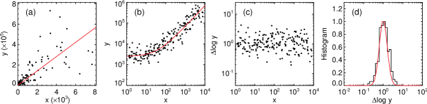
Figure 1.— Correlation plots between two lognormal variables, which are linearly dependent on each other, in (a) linear-linear and (b) log-log scales. Two lognormal variables ($x$ and $y$) were assumed to be correlated according to the linear relationship $\left\langle y\right\rangle=70\left\langle x\right\rangle+2500$, which is denoted by the red curves in (a) and (b). The standard deviations of $\log x$ and $\log y$ were assumed to be $\sigma_{\log x}=\sigma_{\log y}=0.2$. (c) The residual $\Delta\log y\equiv\log y-\left\langle\log y\right\rangle$ versus $\log x$, and (d) the histogram of $\Delta\log y$. The red curve in (d) shows a lognormal function with $\sigma_{\log y}=0.2$.

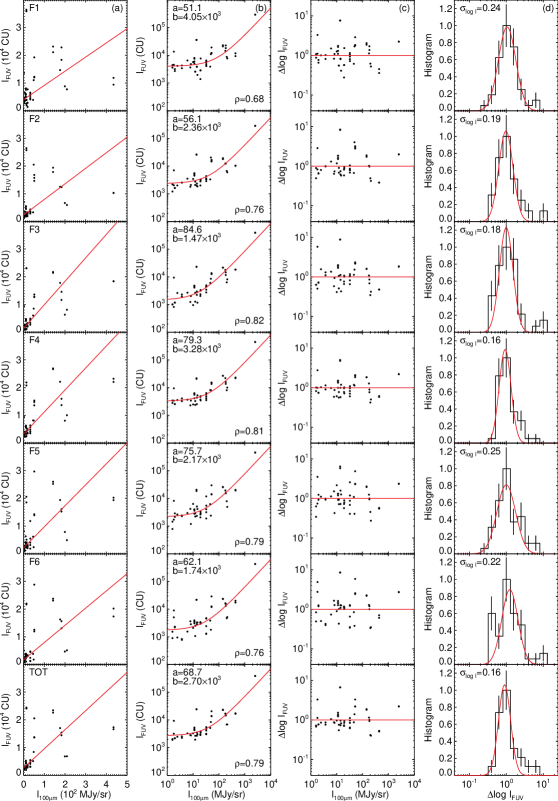
Figure 2.— Correlation plots between the diffuse FUV-S intensity obtained using FUSE and the 100 $\mu$m intensity: (a) $I_{{\rm FUV}}$ versus $I_{{\rm IR}}$, (b) $\log I_{{\rm FUV}}$ versus $\log I_{{\rm IR}}$, (c) $\Delta\log I_{{\rm FUV}}\equiv\log I_{{\rm FUV}}-\left\langle\log I_{{\rm FUV}}\right\rangle$ versus $\log I_{{\rm IR}}$, and (d) the probability distribution function of $\Delta\log I_{{\rm FUV}}$. The red curves in (a) and (b) are linear regression lines. The best-fit parameters $a$ and $b$, and the Pearson’s correlation coefficients are also shown in (b). The best-fit lognormal function of $\Delta\log I_{{\rm FUV}}$ is shown in red in (d). Here, CU represents the continuum unit (photons cm^-2 s^{-1 -1} sr^-1).

Figure 3.— Correlation plots between the diffuse FUV-S intensity obtained using FUSE and the TD-1 SEDI. The linear-linear plots are shown in the first and second columns; the log-log plots are shown in the third and fourth columns. The Pearson’s correlation coefficients are also shown in the third and fourth columns.

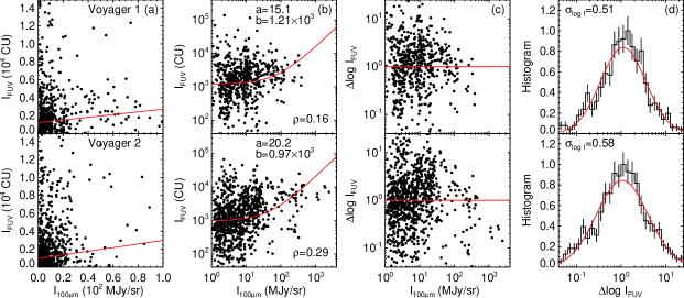
Figure 4.— Correlation plots between the diffuse FUV-S intensity obtained using Voyager and the 100 $\mu$m intensity: (a) $I_{{\rm FUV}}$ versus $I_{{\rm IR}}$, (b) $\log I_{{\rm FUV}}$ versus $\log I_{{\rm IR}}$, (c) $\Delta\log I_{{\rm FUV}}\equiv\log I_{{\rm FUV}}-\left\langle\log I_{{\rm FUV}}\right\rangle$ versus $\log I_{{\rm IR}}$, and (d) the probability distribution function of $\Delta\log I_{{\rm FUV}}$. The red curves in (a) and (b) are the linear regression lines. The best-fit parameters $a$ and $b$, and the Pearson’s correlation coefficients are also shown in (b). The best-fit lognormal function of $\Delta\log I_{{\rm FUV}}$ is shown in red in (d).

Figure 5.— Correlation plots between the diffuse FUV-S intensity obtained using Voyager and the TD-1 SEDI. The linear-linear plots are shown in the first column; the log-log plots are shown in the second column. The Pearson’s correlation coefficients are also shown in the second column.

Figure 6.— Distribution of the standard deviations ($\sigma_{\log N}$ or $\sigma_{\ln N}$) of the dust column density ($N$) derived from various molecular clouds. The standard deviations from individual molecular clouds are also shown; their $y$-values were chosen arbitrarily for clarity. The standard deviations derived from the FUV-S and FUV-L continuum background are also shown.

References

- Belyaev et al. (1971) Belyaev, V. P., Kurt, V. G., Melioranskii, A. S., et al. 1971, Cosmic Research, 8, 677
- Berkhuijsen & Fletcher (2008) Berkhuijsen, E. M., & Fletcher, A. 2008, MNRAS, 390, L19
- Bixler et al. (1984) Bixler, J., Bowyer, S., & Grewing, M. 1984, A&A, 141, 422
- Boulanger & Pérault (1988) Boulanger, F., & Pérault, M. 1988, ApJ, 330, 964
- Bowyer (1991) Bowyer, S. 1991, ARA&A, 29, 59
- Burkhart & Lazarian (2012) Burkhart, B., & Lazarian, A. 2012, ApJ, 755, L19
- Cox & Mezger (1989) Cox, P., & Mezger, P. G. 1989, A&AR, 1, 49
- Deharveng et al. (1982) Deharveng, J. M., Joubert, M., & Barge, P. 1982, A&A, 109, 179
- Edelstein et al. (2000) Edelstein, J., Bowyer, S., & Lampton, M. 2000, ApJ, 539, 187
- Elmegreen (2002) Elmegreen, B. G. 2002, ApJ, 564, 773
- Federrath et al. (2008) Federrath, C., Klessen, R. S., & Schmidt, W. 2008, ApJ, 688, L79
- Federrath et al. (2009) Federrath, C., Klessen, R. S., & Schmidt, W. 2009, ApJ, 692, 364
- Federrath et al. (2010) Federrath, C., Roman-Duval, J., Klessen, R. S., Schmidt, W., & Mac Low, M.-M. 2010, A&A, 512, A81
- Froebrich & Rowles (2010) Froebrich, D., & Rowles, J. 2010, MNRAS, 406, 1350
- Henry (1973) Henry, R. C. 1973, ApJ, 179, 97
- Hill et al. (2008) Hill, A. S., Benjmin, R. A., Kowal, G., et al. 2008, ApJ, 686, 363
- Holberg (1986) Holberg, J. B. 1986, ApJ, 311, 969
- Hurwitz et al. (1991) Hurwitz, M., Bowyer, S., & Martin, C. 1991, ApJ, 372, 167
- Joubert et al. (1983) Joubert, M., Masnou, J. L., Lequeux, J., Deharveng, J. M., & Cruvellier, P., 1983, ApJ, 338, 677
- Kainulainen et al. (2009) Kainulainen, J., Beuther, H., Henning, T., & Plume, R. 2009, A&A, 508, L35
- Klessen (2000) Klessen, R. S. 2000, ApJ, 535, 869
- Lada et al. (1994) Lada, C. J., Lada, E. A., & Clemens, D. P., & Bally, J. 1994, ApJ, 429, 694
- Lombardi et al. (2006) Lombardi, M., Alves, J., & Lada, C. J. 2006, A&A, 454, 781
- Lombardi et al. (2008) Lombardi, M., Alves, J., & Lada, C. J. 2008, A&A, 489, 143
- Miville-Deschênes & Lagache (2005) Miville-Deschênes, M.-A., & Lagache, G. 2005, ApJS, 157, 302
- Moos et al. (2000) Moos, H. W., Cash, W. C., Cowie, L. L., et al. 2000, ApJ, 583, L1
- Murthy et al. (1999) Murthy, J., Hall, D., Earl, M., Henry, R. C., & Holberg, J. B. 1999, ApJ, 522, 904
- Murthy et al. (1991) Murthy, J., Henry, R. C., & Holberg, J. B. 1991, ApJ, 383, 198
- Murthy et al. (2012) Murthy, J., Henry, R. C., & Holberg, J. B. 2012, ApJS, 199, 11
- Murthy et al. (2010) Murthy, J., Henry, R. C., & Sujatha, N. V. 2010, ApJ, 724, 1389
- Murthy & Sahnow (2004) Murthy, J., & Sahnow, D. J. 2004, ApJ, 615, 315
- Nordlund & Padoan (1999) Nordlund, Å., & Padoan, J. 1999, in Interstellar Turbulence, ed. J. Franco & A. Carraminana (Cambridge: Cambridge University Press), 218
- Opal & Weller (1984) Opal, C. B., & Weller, C. S. 1984, ApJ, 282, 445
- Ostriker et al. (2001) Ostriker, E. C., Stone, J. M., & Gammie, C. F. 2001, ApJ, 546, 980
- Padoan et al. (1997) Padoan, P., Jones, B. J. T., & Nordlund, Å. 1997, ApJ, 474, 730
- Paresce & Bowyer (1976) Paresce, F., & Bowyer, S. 1976, ApJ, 207, 432
- Paresce et al. (1980) Paresce, F., McKee, C. F., & Bowyer, S. 1980, ApJ, 240, 387
- Park et al. (2012) Park, S.-J., Min, K.-W., Seon, K.-I., et al. 2012, ApJ, 754, 10
- Pérault et al. (1991) Pérault, M., Lequeux, J., Hanus, M., & Joubert, M. 1991, A&A, 246, 243
- Reynolds (1992) Reynolds, R. J. 1992, ApJ, 392, L35
- Sandel et al. (1979) Sandel, B. R., Shemansky, D. E., & Broadfoot, A. L. 1979, ApJ, 227, 808
- Schiminovich et al. (2001) Schiminovich, D., Friedman, P. G., Martin, C., & Morrissey, P. F. 2001, ApJ, 563, L161
- Schlegel et al. (1998) Schlegel, D. J., Finkbeiner, D. P., & Davis, M. 1998, ApJ, 500, 525
- Schneider et al. (2013) Schneider, N., Andre, P., Könyves, V., et al. 2013, ApJ, 766, L17
- Seon (2009) Seon, K.-I. 2009, ApJ, 703, 1159
- Seon (2012) Seon, K.-I. 2012, ApJ, 761, L17
- Seon et al. (2011a) Seon, K.-I., Edelstein, J., Korpela, E. J., et al. 2011a, ApJS, 196, 15
- Seon et al. (2011b) Seon, K.-I., Witt, A., Kim, I.-J., et al. 2011b, ApJ, 743, 188
- Thompson et al. (1978) Thompson, G. I., Nandy, K., Jamar, C., et al. 1978, Catalogue of Stellar Ultraviolet Fluxes. A Compilation of Absolute Stellar Fluxes Measured by the Sky Survey Telescope (S2/68) aboard the ESRO Satellite TD-1 (London: Sci. Res. Council)
- Vázquez-Semadeni (1994) Vázquez-Semadeni, E. 1994, ApJ, 423, 681
- Wada & Norman (2001) Wada, K., & Norman, C. A. 2001, ApJ, 547, 172
- Witt et al. (1997) Witt, A. N., Friedmann, B. C., & Sasseen, T. P. 1997, 481, 809