Strong coupling of optical nanoantennas and atomic systems

Abstract

An optical nanoantenna and adjacent atomic systems are strongly coupled when an excitation is repeatedly exchanged between these subsystems prior to its eventual dissipation into the environment. It remains challenging to reach the strong coupling regime but it is equally rewarding. Once being achieved, promising applications as signal processing at the nanoscale and at the single photon level would immediately come into reach. Here, we study such hybrid configuration from different perspectives. The configuration we consider consists of two identical atomic systems, described in a two-level approximation, which are strongly coupled to an optical nanoantenna. First, we investigate when this hybrid system requires a fully quantum description and provide a simple analytical criterion. Second, a design for a nanoantenna is presented that enables the strong coupling regime. Besides a vivid time evolution, the strong coupling is documented in experimentally accessible quantities, such as the extinction spectra. The latter are shown to be strongly modified if the hybrid system is weakly driven and operates in the quantum regime. We find that the extinction spectra depend sensitively on the number of atomic systems coupled to the nanoantenna.

I Introduction

Metallic optical nanoantennas have proven perfect in tailoring light-matter interactions at the nanoscale. They allow to drastically change the spontaneous emission rates of adjacent atomic systems or their radiation properties, see e.g. Refs. Anger et al. (2006); Pfeiffer et al. (2010); Curto et al. (2010); Zhu et al. (2012); Filter et al. (2013); Mohtashami and Koenderink (2013). Although the modified light-matter interaction manifests in a multitude of phenomena, all of them are eventually promoted by the same underlying principle, that metallic optical nanoantennas can support strongly localized surface plasmon polaritons. This is at the heart of all observations and entails that their coupling to far-field radiation and quantum systems can be engineered on purpose Novotny and van Hulst (2011); Rogobete et al. (2007).

Recent advances in nanotechnology eventually permitted to fabricate nanoantennas with a precision down to the atomic scale Kern et al. (2012). This implies that a precise arrangement of e.g. quantum dots, molecules, or atoms close to a carefully designed nanoantenna is feasible. It has been already shown that in such situations remarkable new phenomena can be expected where the huge enhancement of dipole-forbidden transitions in the gap of a dimer nanoantenna may serve as a representative example Kern and Martin (2012); Filter et al. (2012). The tremendous spatial localization of the plasmonic mode permits a strong coupling of quantum systems to nanoantennas. The strong coupling regime is characterized by a transition from irreversible spontaneous emission and nonradiative damping processes to a reversible energy exchange between nanoantenna and atomic system. Such a behavior has been reported for cavities operating in the infrared and visible spectral domain Yoshie et al. (2004); Reithmaier et al. (2004); Aoki et al. (2006). To achieve strong coupling is of paramount importance with respect to applications in deterministic quantum computation and for high-power emission of nonclassical light into predefined directions.

Fig. 1: A general scheme of the considered hybrid system. A nanoantenna is strongly coupled to two atoms and excited by an external driving field.

In our contribution we want to go one step further and consider two atoms, rather than a single, isolated one, strongly coupled to a nanoantenna. The aim is to demonstrate that in this case strong coupling effects appear more pronounced where one purpose of the nanoantenna is to strongly increase the interaction between both atoms. Moreover, the structure is highly interesting since a much larger splitting of the energy levels of the hybrid system may be anticipated when compared to that of bare atoms isolated from the nanoantenna. Perspectively, this may suggest an alternative route towards artificial atoms with engineered energy levels. Furthermore, the properties of the hybrid system are shown to sensitively depend on the number of atoms or molecules involved, paving the way for ultra-sensitive devices operating on the single molecule level.

Moreover, besides being of importance from an applied perspective, the setup is essential for basic science since it constitutes a system of rich dynamics that can be operated in different regimes where each regime requires a well-adapted approach to fully grasp its properties. Specifically, the nanoantennas themselves may be described at different levels of approximation.

The simplest approach is to consider the nanoantenna as a passive system which can significantly influence the atoms’ dynamics whereas the properties of the nanoantenna remain unaffected. If such approximation holds, the nanoantenna is treated as a classical harmonic oscillator as frequently done in the literature Yan et al. (2008); Artuso et al. (2011). This simplifies the treatment considerably but prevents the observation of effects associated with the quantum nature of the nanoantenna like Rabi splitting or anti-bunching of its emitted light Meystre and Sargent (1999).

On the contrary, one may account for the full dynamics of the electrons inside the nanoantenna. Such an exhaustive treatment is required if the atoms are placed only a few angstroms off the nanoantenna such that electron-spill-out and quantum tunneling effects become relevant Zuloaga et al. (2010); Manjavacas et al. (2011). However, these effects have not to be considered in most experimentally accessible situations.

In-between, however, lies a regime where the nanoantenna can be considered as a harmonic oscillator but which requires a proper quantization Trügler and Hohenester (2008); Waks and Sridharan (2010); Dzsotjan et al. (2011); Zhang and Govorov (2011); Hümmer et al. (2013). The approach permits the description of the rich quantum behavior of the hybrid system. It is especially useful to study effects at low power levels where only a few photons are involved. However, it is a priori not clear whether such elaborated approach is necessary or whether the semiclassical treatment is already sufficient.

Therefore, at first we will develop both a semiclassical and a fully quantum theory for the problem where an atom described in a two-level approximation is coupled to an optical nanoantenna. In Section III we are going to compare the results of both approaches and we will derive an unambiguous criterion that can be used to decide, on the base of experimentally accessible quantities, which of the two approaches is necessary. Second, in Section IV we will explicitly discuss the design of a nanoantenna that can be operated in the strong coupling regime. After that, in Section V we are going to study the impact of the strong coupling on the extinction spectra of a hybrid system where two atoms are coupled to the optical nanoantenna. We will find that the presence of the atoms strongly affects both absorption and scattering properties of the hybrid system. After concluding on our findings we will provide in elaborated appendices details of our calculations and results that support our conclusions from the main body of the manuscript. In App. A the equations of motion for the semiclassical formulation will be derived. Appendix B details our method to calculate the coupling constants of the nanoantenna to the atoms and to the driving field from numerical simulations. Also, the estimation for the radiative and nonradiative decay rates of the nanoantenna will be given. In App. C, in the framework of the fully quantum approach the eigenstates and -energies of the hybrid system are evaluated in detail.

II Model

We consider two identical two-level systems. We refer to them as atoms, but they could equally describe molecules, quantum dots, NV centres in diamond, etc.Wolters et al. (2012). The two-level-systems shall be symmetrically placed next to a mirror-symmetric nanoantenna that is excited with a driving field propagating along the symmetry axis. Schematically, the situation is shown in Fig. 1. This high symmetry configuration has been chosen for the sake of a reasonable simplicity in our treatment but does not constitute any limitation.

As discussed above, the theoretical description of such a system may be performed in several approximations. In subsection II.1 we consider a fully quantum model including a quantum description of the nanoantenna itself. In practice, such approach requires a considerable numerical effort, unless the excitation field is rather weak and the total system remains approximately at the single excitation level. A considerable simplification and limitation of numerical efforts is provided by a mean-field approximation, where the electromagnetic field is described classically Słowik et al. (2012). This semi-classical treatment will be given in subsection II.2. Both models will be compared in the succeeding section.

II.1 Fully quantum approach

In the fully quantum approach, we regard the nanoantenna as a single mode quantum harmonic oscillator. Then the Hamiltonian in the rotating frame takes the following form within the rotating wave approximation Meystre and Sargent (1999):

$$H = \frac{\hbar\,\Delta\omega_{0}}{2}\sum_{j=1}^{N_{\mathrm{tls}}}\left(\sigma_{z}^{(j)}+1\!\!1\right)+\hbar\Delta\omega_{\mathrm{na}}a^{\dagger}a$$

$$-\hbar\kappa\sum_{j=1}^{N_{\mathrm{tls}}}\left(\sigma_{+}^{(j)}a+a^{\dagger}\sigma_{-}^{(j)}\right)-\hbar\Omega\left(a+a^{\dagger}\right),$$

with $\Delta\omega_{0}=\omega_{0}-\omega_{\mathrm{dr}}$, $\Delta\omega_{\mathrm{na}}=\omega_{\mathrm{na}}-\omega_{\mathrm{dr}}$. Here, ${N_{\mathrm{tls}}}=2$ is the number of identical atoms, and $\omega_{0}$ corresponds to their transition frequency. The operators $\sigma_{z}^{(j)}=|e^{(j)}\rangle\langle e^{(j)}|-|g^{(j)}\rangle\langle g^{(j)}|$ represent the population inversion in the $j^{\mathrm{th}}$ two-level system, and $\sigma_{+}^{(j)}=|e^{(j)}\rangle\langle g^{(j)}|$ and $\sigma_{-}^{(j)}={\sigma_{+}^{(j)}}^{\dagger}$ are the corresponding creation and annihilation operators of atomic excitation. As usual, $\{|e^{(j)}\rangle\text{ and }|g^{(j)}\rangle\}$ denote the excited and ground state of the $j^{\mathrm{th}}$ two-level system. The symbols $a$ and $a^{\dagger}$ stand for the annihilation and creation operator of the nanoantenna mode, respectively. Several approximations have been made here. For simplicity, only the dipolar transitions in the atoms have been taken into account. In case when such approximation is not valid, a treatment like the one described in Ref. Lembessis and Babiker (2013), should be applied. Treatment of the nanoantenna as a single-mode harmonic oscillator is also an approximation. It is assumed that a single resonance dominates the nanoantenna spectrum around the atomic transition frequency, see also Refs. Yan et al. (2008); Filter et al. (2012) and the discussion in Section IV.

We note that the single-mode approach for both the atomic system and the nanoantenna is an approximation taking only the dipolar transitions in the atomic system and the nanoantenna into account, see and App. B.

The nanoantenna is coherently driven by an external laser beam, assumed to be monochromatic at frequency $\omega_{\mathrm{dr}}$. The driving field intensity is related to the Rabi frequency $\Omega$, which is here taken real for simplicity, see App B. The coupling constant between atom and nanoantenna is given by $\kappa$, identical for both atoms because of their symmetric placement. Note that $\kappa$ can be assumed constant, if the transition frequency of the atoms is close to the broad resonance of the nanoantenna of central frequency $\omega_{\mathrm{na}}$. We neglect the free-space interaction of the atoms, i.e. the dipole-dipole interaction in the absence of the nanoantenna, because it is considerably weaker than the interaction of the atoms due to the nanoantenna. We also neglect the direct coupling of the driving field to the atoms, as, again, it is much weaker than the nanoantenna’s scattered field at the position of the atoms.

The dynamics of the hybrid system is described by the Lindblad-Kossakowski equation Meystre and Sargent (1999):

$$\mathrm{i}\hbar\dot{\rho} = \left[H,\rho\right]+\mathrm{i}\mathcal{L}_{\mathrm{na}}\left(\rho\right)+\mathrm{i}\mathcal{L}_{\mathrm{tls}}\left(\rho\right),$$ (2)

where $\rho$ is the density operator of the hybrid system and $\mathcal{L}_{\mathrm{na,tls}}\left(\rho\right)$ are Lindblad operators responsible for losses in the nanoantenna and the atoms, respectively, given by

$$\mathcal{L}_{\mathrm{na}}\left(\rho\right) = -\hbar\Gamma\left(a^{\dagger}a\rho+\rho a^{\dagger}a-2a\rho a^{\dagger}\right),$$ (3)

$$\mathcal{L}_{\mathrm{tls}}\left(\rho\right) = -\frac{1}{2}\hbar\Gamma_{\mathrm{fs}}\sum_{j=1}^{N_{\mathrm{tls}}}\left(\sigma_{+}^{(j)}\sigma_{-}^{(j)}\rho+\rho\sigma_{+}^{(j)}\sigma_{-}^{(j)}\right.$$

$$\left.-2\sigma_{-}^{(j)}\rho\sigma_{+}^{(j)}\right)$$

$$+\frac{1}{2}\hbar\Gamma_{\mathrm{d}}\sum_{j=1}^{N_{\mathrm{tls}}}\left(\sigma_{z}^{(j)}\rho\sigma_{z}^{(j)}-\rho\right).$$

In the above expressions $\Gamma=\Gamma_{\mathrm{r}}+\Gamma_{\mathrm{nr}}$ describes radiative and nonradiative losses by the nanoantenna. The free-space spontaneous emission rate of a single two-level system is given by $\Gamma_{\mathrm{fs}}$, whereas $\Gamma_{\mathrm{d}}$ is the rate of pure dephasing. An example of the latter would be the interactions with phonons in quantum dots that affect the coherence but not the population distribution Heiss et al. (2007). Typically, the radiative and nonradiative losses in the metallic nanoparticle are much stronger than all losses in the atoms.

II.2 Semiclassical approach

In the preceding subsection we have formally introduced a fully quantum description of the atoms coupled to a nanoantenna. Now the same physical situation will be considered but the description of the nanoantenna will be approximated by a classical equation of motion. The state of the atomic system may then be described by its density operator which we denote as $\rho^{\mathrm{sc}}$. Its evolution follows the Lindblad-Kossakowski equation

$$\mathrm{i}\hbar\dot{\rho}^{\mathrm{sc}}=\left[H^{\mathrm{sc}},\rho^{\mathrm{sc}}\right]+\mathrm{i}\mathcal{L}_{\mathrm{tls}}\left(\rho^{\mathrm{sc}}\right),$$ (5)

with the semiclassical Hamiltonian Meystre and Sargent (1999)

$$H^{\mathrm{sc}} = \frac{\hbar\Delta\omega_{0}}{2}\sum_{j=1}^{N_{\mathrm{tls}}}\left(\sigma_{z}^{(j)}+1\!\!1\right)$$

$$-\hbar\kappa\sum_{j=1}^{N_{\mathrm{tls}}}\left[\sigma_{+}^{(j)}\alpha\left(t\right)+\alpha^{\star}\left(t\right)\sigma_{-}^{(j)}\right]\ .$$

For the sake of comparison to the fully quantum Hamiltonian $H$, we denote the Rabi frequency of the scattered field by $\kappa\alpha\left(t\right)$, with the classical dimensionless amplitude $\alpha\left(t\right)\in\mathbb{C}$.

The time-dependent dipole moment of each atom acts naturally as electrodynamic source. Thus, the overall field is a superposition of contributions from the atoms and the nanoantenna. Usually the field generated by the $j^{\mathrm{th}}$ atom is expressed by its mean transition dipole moment, $\mathbf{E}\left(\mathbf{r},t\right)\propto\langle\mathbf{d}^{(j)}\rangle=\mathbf{d}_{\mathrm{ge}}^{\mathrm{(j)}}{\rho_{\mathrm{eg}}^{\mathrm{sc}}}^{(j)}$ Yan et al. (2008), where ${\rho_{\mathrm{mn}}^{\mathrm{sc}}}^{(j)}={{\rho_{\mathrm{nm}}^{\mathrm{sc}}}^{(j)}}^{\star}=\langle m|{\rho^{\mathrm{sc}}}^{(j)}|n\rangle$ is an element of the reduced density matrix of the $j^{\mathrm{th}}$ atom, and the asterisk stands for the complex-conjugate. Similarly, $\mathbf{d}_{\mathrm{ge}}^{\mathrm{(j)}}=\langle g^{(j)}|\mathbf{d}^{\mathrm{(j)}}|e^{(j)}\rangle$ corresponds the matrix element of the $j^{\mathrm{th}}$ atom dipole moment operator. As derived in App. A, the evolution equation of the field in the slowly-varying envelope approximation $|\dot{\alpha}|\ll|\alpha\omega_{\mathrm{dr}}|$ and for $\Gamma\ll\omega_{\mathrm{dr}}$ is given by

$$\dot{\alpha}\left(t\right) = -\left(\Gamma+i\Delta\omega_{\mathrm{na}}\right)\alpha\left(t\right)$$

$$+i\left[\kappa\sum_{j}{\rho_{eg}^{\mathrm{sc}}}^{(j)}(t)+\Omega\right].$$

Such a description is an approximation which turns out to be valid just for very weak excitations as we will show in the following section.

III Comparison of semiclassical and fully quantum approaches

One of the main issues addressed in this paper concerns the identification of conditions where the semiclassical and the fully quantum approaches yield equivalent results. To this end, we will consider the simplest scenario where a single atom is coupled to the nanoantenna at first. We will directly compare the evolution equations of the atomic operators in the fully quantum approach, obtained in the Heisenberg picture, with the corresponding ones of the atomic density matrix and of the field amplitude in the semiclassical approach. A limit will be identified where both approaches agree to a good approximation. An interpretation in terms of correlation functions will also be provided.

As we will show, the very source of discrepancies between both approaches is the interaction term proportional to $\kappa$, which we will now focus on. For this reason we consider for a while the simplified lossless case, and also set $\Omega=0$, but assume that the excitation is initially present in the coupled system. For instance, the atom is initially excited and/or photons are present in the field of the nanoantenna.

Directly from the Heisenberg equation $\dot{A}=-i/\hbar[A,H]+\frac{\partial A}{\partial t}$, which describes the evolution of any operator $A$, we obtain the evolution of the field annihilation operator in the rotating frame in the fully quantum picture:

$$\dot{a}\left(t\right)=-i\Delta\omega_{\mathrm{na}}a\left(t\right)+i\kappa\sigma_{-}\left(t\right),$$ (8)

and of the atomic operators:

$$\dot{\sigma}_{z}\left(t\right) = 2\mathrm{i}\kappa\left[\sigma_{+}\left(t\right)a\left(t\right)-a^{\dagger}\left(t\right)\sigma_{-}\left(t\right)\right],$$ (9)

$$\dot{\sigma}_{-}\left(t\right) = -\mathrm{i}\Delta\omega_{0}\sigma_{-}\left(t\right)-\mathrm{i}\kappa\sigma_{z}\left(t\right)a\left(t\right).$$ (10)

The first equation can be formally integrated to give

$${a}\left(t\right) = a\left(0\right)e^{-i\Delta\omega_{\mathrm{na}}t}$$

$$+i\int_{0}^{t}\kappa\sigma_{-}\left(t^{\prime}\right)e^{-i\Delta\omega_{\mathrm{na}}\left(t-t^{\prime}\right)}dt^{\prime}.$$

Inserting this resut into equations (9-10) leads to the following evolution equations for the expectation values:

$$\langle\dot{\sigma}_{z}\left(t\right)\rangle = 2\mathrm{i}\kappa\left[\langle\sigma_{+}\left(t\right)a\left(0\right)\rangle e^{-i\Delta\omega_{\mathrm{na}}t}-\mathrm{c.c.}\right]$$

$$-2\kappa^{2}\int_{0}^{t}\langle\sigma_{+}\left(t\right)\sigma_{-}\left(t^{\prime}\right)\rangle e^{-i\Delta\omega_{\mathrm{na}}\left(t-t^{\prime}\right)}dt^{\prime}$$

$$-2\kappa^{2}\int_{0}^{t}\langle\sigma_{+}\left(t^{\prime}\right)\sigma_{-}\left(t\right)\rangle e^{i\Delta\omega_{\mathrm{na}}\left(t-t^{\prime}\right)}dt^{\prime}$$

$$\langle\dot{\sigma}_{-}\left(t\right)\rangle = -\mathrm{i}\Delta\omega_{0}\langle\sigma_{-}\left(t\right)\rangle$$

$$-\mathrm{i}\kappa\langle\sigma_{z}\left(t\right)a\left(0\right)\rangle e^{-i\Delta\omega_{\mathrm{na}}t}$$

$$+\kappa^{2}\int_{0}^{t}\langle\sigma_{z}\left(t\right)\sigma_{-}\left(t^{\prime}\right)\rangle e^{-i\Delta\omega_{\mathrm{na}}\left(t-t^{\prime}\right)}dt^{\prime},$$

where $\mathrm{c.c.}$ stands for the complex-conjugate. We consider here the evolution of expectation values of the atomic operators because it can be directly compared with the evolution of the corresponding elements of the density matrix, i.e. $\langle\sigma_{z}(t)\rangle=\rho_{ee}^{\mathrm{sc}}(t)-\rho_{gg}^{\mathrm{sc}}(t)$, $\langle\sigma_{-}(t)\rangle=\rho_{eg}^{\mathrm{sc}}(t)$.

Similarly, in the semiclassical description we integrate equation (II.2) with $\Gamma$ and $\Omega$ set to zero. Next, we insert it into the Lindblad-Kossakowski equation (5) with $\Omega=0$ and $\Gamma_{\mathrm{fs}}=\Gamma_{\mathrm{d}}=0$, to arrive at:

$$\dot{\rho}_{ee}^{\mathrm{sc}}-\dot{\rho}_{gg}^{\mathrm{sc}} = 2\mathrm{i}\kappa\left[\rho_{ge}^{\mathrm{sc}}\left(t\right)\alpha\left(t\right)-\alpha^{\star}\left(t\right)\rho_{eg}^{\mathrm{sc}}\left(t\right)\right]$$

$$= 2\mathrm{i}\kappa\left[\rho_{ge}^{\mathrm{sc}}\left(t\right)\alpha\left(0\right)e^{-\mathrm{i}\Delta\omega_{\mathrm{na}}t}-\mathrm{c.c.}\right]$$

$$-2\kappa^{2}\int_{0}^{t}\rho_{ge}^{\mathrm{sc}}\left(t\right)\rho_{eg}^{\mathrm{sc}}\left(t^{\prime}\right)e^{-i\Delta\omega_{\mathrm{na}}\left(t-t^{\prime}\right)}dt^{\prime}$$

$$-2\kappa^{2}\int_{0}^{t}\rho_{ge}^{\mathrm{sc}}\left(t^{\prime}\right)\rho_{eg}^{\mathrm{sc}}\left(t\right)e^{i\Delta\omega_{\mathrm{na}}\left(t-t^{\prime}\right)}dt^{\prime}$$

$$\dot{\rho}_{eg}^{\mathrm{sc}} = -\mathrm{i}\Delta\omega_{0}{\rho}_{eg}^{\mathrm{sc}}-\mathrm{i}\kappa\alpha\left(t\right)\left[\rho_{ee}^{\mathrm{sc}}\left(t\right)-\rho_{gg}^{\mathrm{sc}}\left(t\right)\right]$$

$$= -\mathrm{i}\Delta\omega_{0}{\rho}_{eg}^{\mathrm{sc}}$$

$$-\mathrm{i}\kappa\left[\rho_{ee}^{\mathrm{sc}}\left(t\right)-\rho_{gg}^{\mathrm{sc}}\left(t\right)\right]\alpha\left(0\right)e^{-i\Delta\omega_{\mathrm{na}}t}$$

$$+\kappa^{2}\int_{0}^{t}\left[\rho_{ee}^{\mathrm{sc}}\left(t\right)-\rho_{gg}^{\mathrm{sc}}\left(t\right)\right]\rho_{eg}^{\mathrm{sc}}\left(t^{\prime}\right)\times$$

$$\times e^{-i\Delta\omega_{\mathrm{na}}\left(t-t^{\prime}\right)}dt^{\prime}.$$

Now by directly comparing the equations obtained in both descriptions we note that the semiclassical approach leads to nonlinear terms of the type $\rho_{ij}^{\mathrm{sc}}(t)\rho_{kl}^{\mathrm{sc}}(t^{\prime})$ or, equivalently, $\langle\sigma_{p}(t)\rangle\langle\sigma_{q}(t^{\prime})\rangle$, with $i,j,k,l=e,g$ and $p,q=z,+,-$. On the other hand, from the analysis of the Heisenberg equations of motion, i.e. without the mean field approximation, we can see that terms such as $\langle\sigma_{p}(t)\sigma_{q}(t^{\prime})\rangle$ appear in the equations of motion instead Chen et al. (2013).

Both results are only equivalent if the atomic operators are uncorrelated, i.e. if $\langle\sigma_{p}(t)\sigma_{q}(t^{\prime})\rangle\approx\langle\sigma_{p}(t)\rangle\langle\sigma_{q}(t^{\prime})\rangle$. A similar problem has been investigated in Ref. Dorner and Zoller (2002), where the authors use a harmonic oscillator model for a two-level system and demonstrate that the condition of uncorrelated system operators is fulfilled for a harmonic oscillator initially it its ground state. A harmonic oscillator is indeed a good model of a two-level system if its first excited state occupation probability is small, and the doubly and higher excited states are not relevant.

Likewise, a two-level system is a good model for a harmonic oscillator if the system is approximately in its ground state. Then the bosonic commutation rule can be recovered for the annihilation and creation operators $\left[\sigma_{-},\sigma_{+}\right]=-\sigma_{z}\approx 1$ and one may apply the result of Ref. Dorner and Zoller (2002) to the case of a two-level system. Moreover, only in such case the two-level system is a source of coherent light, which can be accurately described by the semiclassical approximation. Only if the condition of uncorrelated system operators holds true, i.e. the two-level system has to stay approximately in its ground state throughout the entire evolution, the mean field approximation, and so the semiclassical approach, are valid Waks and Sridharan (2010). It is important to note that the applicability of this restriction does not depend on the coupling strength. Furthermore, our condition holds in general for any situation where atomic systems interact with light rather than only for coupling of two-level systems to nanoantennas considered here.

For simulations it is often crucial to find a strict criterion for the validity of the semiclassical approximation. Such a criterion can be found by deriving the steady-state solution of equations (III), where the driving field or loss rates are no longer assumed to be zero. The assumption that must be fulfilled for the semiclassical approximation to be valid is that the excited state occupation of either atomic system is small, i.e. $1\approx\rho_{gg}^{\mathrm{sc}}\gg\rho_{ee}^{\mathrm{sc}}$. Then, we find

$$\rho_{ee}^{\mathrm{sc}} \approx \frac{2\Gamma_{\mathrm{dec}}}{\Gamma_{\mathrm{fs}}}\frac{\kappa^{2}\Omega^{2}}{D}\ll 1,$$ (16)

$$D = (\Gamma_{\mathrm{dec}}^{2}+\Delta\omega_{0}^{2})(\Gamma^{2}+\Delta\omega_{\mathrm{na}}^{2})$$

$$+2(\Gamma_{\mathrm{dec}}\Gamma-\Delta\omega_{0}\Delta\omega_{\mathrm{na}})\kappa^{2}+\kappa^{4},$$

where $\Gamma_{\mathrm{dec}}=\frac{1}{2}\Gamma_{\mathrm{fs}}+\Gamma_{\mathrm{d}}$ is the total decoherence rate of an atom, which includes contributions from spontaneous emission and pure dephasing processes. In the resonant case with $\omega_{\mathrm{dr}}=\omega_{\mathrm{na}}=\omega_{0}$, the validity criterion for the semiclassical approximation simplifies to

$$\rho_{ee}^{\mathrm{sc}} \approx \frac{2\Gamma_{\mathrm{dec}}}{\Gamma_{\mathrm{fs}}}\frac{\kappa^{2}\Omega^{2}}{(\Gamma_{\mathrm{dec}}\Gamma+\kappa^{2})^{2}}\ll 1.$$ (17)

This condition of weak driving fields is confirmed in numerical simulations using Mathematica 7 Wolfram (1999). The calculations were carried out by numerically solving the Lindblad-Kossakowski equation (2) in the fully quantum approach. For the semiclassical approach, Eqs. (5) and (II.2) were numerically solved, respectively.

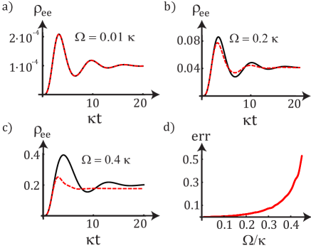
Fig. 2: Excited state occupation probability of the atom vs. normalized time for different Rabi frequencies $\Omega$ of the driving field and $\omega_{\mathrm{dr}}=\omega_{\mathrm{na}}=\omega_{0}$, $\Gamma=0.5\kappa$, $\Gamma_{\mathrm{fs}}=10^{-9}\kappa$, $\Gamma_{\mathrm{d}}=0$. The black solid line corresponds to the semiclassical and the red dashed line to the fully quantum results. (a) For weak driving fields a perfect agreement is obtained. (b, c) For stronger driving fields both the time evolution and the steady state results are incorrectly evaluated in the semiclassical approximation (17). (d) The relative error of the steady-state results grows fast with increasing $\Omega/\kappa$ ratio.

We have performed simulations for different driving strengths assuming $\omega_{\mathrm{dr}}=\omega_{\mathrm{na}}=\omega_{0}$, $\Gamma=0.5\kappa$, $\Gamma_{\mathrm{fs}}=10^{-9}\kappa$, $\Gamma_{\mathrm{d}}=0$. Initially, the atom is assumed to be in its ground state and the field amplitude of the nanoantenna vanishes: $\rho(t=0)=|g\rangle\langle g|\otimes|0\rangle\langle 0|$ is the initial condition for the fully quantum case, whereas $\rho^{\mathrm{sc}}(t=0)=|g\rangle\langle g|$ and $\alpha(t=0)=0$ correspond to that of the semiclassical one. In the fully quantum approach we perform the calculations in a Hilbert space truncated at sufficiently high number $k_{\mathrm{max}}$ of excitations in the nanoantenna. Here it suffices to set $k_{\mathrm{max}}=10$. In Fig. 2, the excited state occupation probability of the atom is compared when calculated in the semiclassical (black solid line) and the fully quantum approach (red dashed line), for increasing intensities of the driving field [panels (a)-(c)]. For weak fields, and thus small excited state occupations, the results are in perfect agreement (a). Slightly stronger fields result in discrepancies in time evolution, but the steady state occupation coincides in both approaches (b). This is no longer the case for rather strong driving fields that result in considerable excitation probabilities of the atom (c). In panel (d) the steady-state relative error, defined as $\mathrm{err}\equiv\left.\left|\rho_{\mathrm{ee}}^{\mathrm{sc}}-\rho_{\mathrm{ee}}\right|/\rho_{\mathrm{ee}}\right|_{t\rightarrow\infty}$, is shown to grow fast with the ratio of the Rabi frequency of the driving field $\Omega$ to the coupling constant $\kappa$.

On more analytical grounds, we can first examine the simplest case where the spontaneous emission is the only source of decoherence, i.e. $\Gamma_{\mathrm{d}}=0$ and $\Gamma_{\mathrm{dec}}=\frac{1}{2}\Gamma_{\mathrm{fs}}$. Then, the prefactor in Eq. (17) is unity because of $2\Gamma_{\mathrm{dec}}/{\Gamma_{\mathrm{fs}}}=1$. Moreover, for small losses Eq. (17) may be further simplified. Then we find a condition for the validity of the semiclassical approach as $\Omega\ll\kappa$. If that condition holds $\rho_{ee}^{\mathrm{sc}}\ll 1$, i.e., the atom will approximately remain in its ground state. If losses dominate, i.e. for atoms weakly coupled to a nanoantenna, the semiclassical approximation can be applied as long as $\Omega\ll\Gamma\Gamma_{\mathrm{fs}}/\kappa$.

If dephasing is additionally present $(\Gamma_{\mathrm{d}}\neq 0)$, the excited state occupation is always increased (not shown) with respect to the case of pure spontaneous emission, which makes condition (17) more difficult to be fulfilled. For small driving field intensities the peak value of the excited-state occupation probability is equal to $\rho_{\mathrm{ee,max}}^{\mathrm{sc}}\approx\Omega^{2}/2\Gamma_{\mathrm{fs}}\Gamma$ and is reached for $\Gamma_{\mathrm{dec}}=\kappa^{2}/\Gamma$. Thus we arrive at a strong worst-case-scenario criterion valid for an arbitrary dephasing rate and an arbitrary coupling strength: $\Omega^{2}\ll\Gamma_{\mathrm{fs}}\Gamma$.

This result may seem counterintuitive. One might have expected that the semiclassical approximation is valid in the limit of sufficiently strong rather than weak fields. This result can be understood as follows. For weak driving fields, in good approximation the atoms are in their ground states. Then, they behave as harmonic oscillators which can be accurately described by the semiclassical approach which is in accordance with the results presented in Ref. Waks and Sridharan (2010). For stronger fields, the approximation of the two-level systems as harmonic oscillators breaks down and consequently the semiclassical approach too. However, for even stronger fields the feedback from the atoms is only of minor relevance. Mathematically, this interaction region can be defined by $|\alpha|^{2}\gg 1$ which naturally leads to $\Omega\gg\Gamma\text{ ,}\kappa$.

IV Design of the nanoantenna

In this section we aim at designing a nanoantenna that allows achieving the strong coupling regime. The latter can be defined by Wallraff et al. (2004)

$$\kappa>\Gamma.$$ (18)

This condition suggests that an excitation is exchanged between the atomic and the nanoantenna subsystems prior to its eventual dissipation into the environment. We assume the decay and decoherence rates in the atoms small in comparison with the losses by the nanoparticle. Slightly differently to Eq. (18) strong coupling might also be defined with regard to the emergence of a dressed state, see Andreani et al. (1999); Savasta et al. (2010).

On our path to a design that allows for the strong coupling regime, we are going to investigate how coupling constants and loss rates can be tailored by varying shape and size of the nanoantenna. As a main result of this section we shall find that strong coupling can be achieved if the characteristic spatial dimensions of the nanoantenna are small. The size of the nanoantenna should not be larger than a few tens of nanometers and the separation of the elements forming the nanoantenna should be of the order of a few nanometers. Small spatial dimensions are eventually the crucial condition since they guarantee sufficiently small mode volumes as required to reach the strong coupling regime. In the following we analyze the nanoantennas in terms of two generic parameters that determine their radiative properties and are frequently exploited while engineering nanoantennas: the nanoantenna efficiency $\eta\equiv\Gamma_{\mathrm{r}}/\Gamma$ and the Purcell factor $F$. The efficiency is a measure for the fraction of radiative energy loss $\Gamma_{\mathrm{r}}$ by the nanoantenna when compared to its total energy loss $\Gamma=\Gamma_{\mathrm{r}}+\Gamma_{\mathrm{nr}}$ Novotny and Hecht (2006). As discussed earlier, the coupling to higher order modes was neglected so far. However, not to artificially overestimate the nanoantenna’s efficiency, we calculate $\eta$ for a nanoantenna excited by dipoles at the positions of the atoms.

The Purcell factor is here understood as a measure for the nanoantenna’s capability to enhance the radiation of a dipole source Bharadwaj et al. (2009). It naturally depends on the position of the source with respect to the nanoantenna. We find the Purcell factor as the ratio of the total energy flux calculated with and without nanoantenna. The latter case corresponds to the free-space emission rate $\Gamma_{\mathrm{fs}}$. Note that the Purcell factor introduced here is different from that used in the context of cavity QED, i.e. the enhancement of the decay rate of an atom Meystre and Sargent (1999); Novotny and Hecht (2006). The decay rate of atoms interacting with a nanoantenna can be enhanced by radiative and/or nonradiative loss channels of the nanoantenna. Both losses coincide only for nanoantennas with the efficiency equal to $1$. Our results prove that there is a trade-off between the nanoantenna efficiency (or the Purcell factor) and the coupling strength that can be achieved with a nanoantenna.

Our electromagnetic simulations were performed with COMSOL MULTIPHYSICS simulation platform where the dispersive permittivity has been fully considered Palik (1985). The methods that we use to compute the coupling constants and loss rates for a specific nanoantenna are described in detail in App. B. Here, we note that the results were obtained using the plane-wave illumination scheme for the nanoantenna. In such scheme almost solely the dipolar mode is excited and dominates the single nanoantenna resonance. The results might thus change in a different, e.g. dipole, illumination scheme, where higher-order modes may in general also contribute to the resonance. However, in case of small nanoparticles, like the ones considered in this paper, this influence can approximately be neglected. Thus, we do not take these higher order modes into account.

Two basic nanoantenna geometries which obey the assumptions made in the introduction are considered from now on: (1) a single or (2) three identical silver nanospheroids with axis lengths $a$ and $b$. For prolate nanospheroids $a>b$ holds. The three-nanospheroid geometry is shown in Fig. 3(a). The nanospheroids are positioned at a distance $r_{0}$ from each other along the $x$ axis of the chosen coordinate system with its origin at the center of the middle nanospheroid.

The reason to compare single- and multiple-nanospheroid geometries is the following: single nanospheroids are easier to fabricate, as the experimentally-demanding narrow gap is not required, and they might be suitable for reaching the strong coupling, as investigated in Trügler and Hohenester (2008); Ge et al. (2013). On the other hand, multiple structures have the potential to confine and enhance fields much stronger when compared to isolated nanospheroids. Furthermore, as we will show below, they are characterized with higher efficiencies and Purcell factors, which makes them more suitable for applications, e.g., as nonclassical light sources Mu and Savage (1992); Maksymov et al. (2012).

To provide a visual impression of the spatial distribution of the enhanced field, we consider a three-nanospheroid design with the largest $\kappa/\Gamma$ ratio: a nanoantenna made of prolate nanospheroids of $a=13.3$ nm, $b=8$ nm, and $r_{0}=2$ nm, subject to the driving field of frequency $\omega_{\mathrm{dr}}=3.37\times 10^{15}\,\mathrm{s^{-1}}$, which is the resonance frequency of the nanoantenna. It is worth noting that an exact resonance with the atomic transition frequency is not crucial because of the broad resonance of the nanoantenna. The driving field propagates along the $y$ direction and is polarized in $x$ direction. In Fig. 3(b) we show the spatial distribution of the absolute value of the $x$-polarized component of the scattered field in the $xy$ plane, normalized to the value of the incoming field. It is the $x$-component of the enhanced field which contributes to the coupling constant $\kappa$, as it is parallel to the assumed direction of the transition dipole moments of the atoms. Only the scattered, not the total (scattered + driving) field is considered here, because the driving field is considerably weaker and its action on the atom can be neglected to a good approximation. This is in accordance with the assumptions made for the Hamiltonians (II.1,II.2), considered in Sec. II.

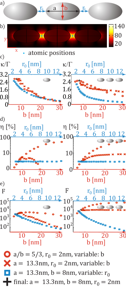
Fig. 3: (a) General scheme of the nanoantenna consisting of three identical nanospheroids of aspect ratio $a/b$, positioned at distance $r_{0}$ from each other. (b) Distribution of the absolute value of the $x$-polarized component of the scattered field (normalized by the value of the incoming field) for three identical nanospheroids with $a=13.3$ nm and $b=8$ nm and separated by $r_{0}=2$ nm. The coupling constant $\kappa$ is proportional to the enhancement of the $x$-polarized scattered field component at the point where an atom is placed (blue dots). (c) $\kappa/\Gamma$ ratio for $d_{\mathrm{ge}}=6\times 10^{-29}$ Cm and various geometrical parameters of the single- (left) and three-spheroid (right) nanoantenna: dependence on size (red circles, constant aspect ratio $a/b=5/3$, $r_{0}=2$ nm), on aspect ratio (red crosses, constant $a=13.3$ nm, $r_{0}=2$ nm), and on distance $r_{0}$ (blue squares, $a=13.3$ nm and $b=8$ nm). The atomic distance from nanoantenna tip is always $r_{0}/2$. (d) Nanoantenna efficiency and (e) Purcell factor, values of parameters as in (c). The proposed design of a three-spheroid nanoantenna that corresponds the scattered field distribution of panel (b), is described in the text and marked in (c)-(e) with the black cross.

For obtaining results displayed in Fig. 3 we scanned the extinction cross-section Bohren and Huffman (1998) of every nanoantenna, subjected to a monochromatic driving field, in the pertinent frequency domain to find its resonance frequency $\omega_{\mathrm{na}}$. We assumed a lossless host medium ($\varepsilon=2.2$). Next we considered a resonantly driven nanoantenna to find both the loss rate $\Gamma$ and the coupling constant $\kappa$ at the positions of the atoms, which is always taken as $r_{0}/2$ and in the case of three nanospheroids it is the point equidistant from two spheroids, as described in App. B. We set the transition dipole moment of an atom to a rather high, but realistic value of $d_{\mathrm{ge}}=6\times 10^{-29}$ Cm.

In Fig. 3(c) the $\kappa/\Gamma$ ratio for nanoantennas of varying size (red circles) and aspect ratio (red crosses) is shown. The essential result is that the strong coupling regime may only be achieved for small nanoantennas (minor axis below $30$ nm in case of three-, and below $20$ nm in case of single-nanospheroid designs). Less important is the rather weak dependence on the aspect ratio $a/b$: the $\kappa/\Gamma$ ratio is larger for prolate objects, as they can confine and enhance the fields stronger than oblate ones. Still, the strong coupling can be achieved even for oblate nanospheroids. However, greater care for the shape must be taken if only one nanospheroid is considered. In the same figure the dependence on the separation distance $r_{0}$ between the nanospheroids is displayed (blue squares). The distance of the atom to the nanospheroid is in each case equal to $r_{0}/2$, so increasing $r_{0}$ means also increasing the distance from the atom to the nanospheroids. This explains why the field enhancement, and consequently the coupling constant $\kappa$, drops with distance $r_{0}$. A strong field enhancement, and thus strong coupling, are obtained if the individual nanospheroids are less than $4$ nm apart from each other. Interestingly, slightly larger atom-nanoantenna distances allow for strong coupling in the single-nanospheroid case.

Next we are going to analyze the efficiencies of the above-considered nanoantennas [see Fig. 3(d)]. According to our investigations, a small size, which is the key for strong coupling, will result in a poor nanoantenna efficiency, however, always larger in the multiple-spheroid case. For nanospheroids of the size at which the strong coupling is reached ($18$ nm in the single- and $30$ nm in the multiple-nanospheroid case) the efficiency reads $24\%$ and $54\%$, respectively, and drops dramatically as the size decreases. In Ref. Bohren and Huffman (1998) such scaling of the size-dependent efficiency has been rigorously derived for spherical particles in terms of scattering and absorption cross sections. The efficiency clearly drops for prolate nanoantennas in the muliple-nanospheroid case. The impact of the adjacent dipoles and of additional nanospheroids on radiative losses and absorption turns out to be marginal, so the efficiencies of the proposed nanoantennas show little dependence on $r_{0}$.

Relatively higher radiative losses in large nanoantennas result in an increase of the Purcell factor [see Fig. 3(d)]. Again, it is the size that determines to a large extent the radiative losses of the nanoparticle. The Purcell factor is almost constant for a varying aspect ratio in the case of multiple-spheroid nanoantennas, but it decreases fast for oblate objects in the case of single spheroids. Naturally, the Purcell factor drops as the distance between the nanoantenna and the dipole source grows, since then their mutual interaction decreases significantly.

We may summarize the above considerations by noting that both single- and multiple-structure geometries are suitable for strong coupling, although due to their ability to confine and enhance fields stronger, three-nanospheroid designs lead to the strong coupling regime at larger nanospheroid sizes. They are also characterized by larger efficiencies and Purcell factors. Therefore, the optimal geometry turns out to be the one always marked with the black cross in Fig. 3 and used for plotting the field distribution in Fig. 3(b). For such design we obtain $\Gamma_{\mathrm{nr}}=7.0\times 10^{13}$ Hz, $\Gamma_{\mathrm{r}}=6.0\times 10^{12}$ Hz. (Once again, we note that small nanoantennas designed for strong coupling turn out to be rather poor emitters: nonradiative losses prevail against radiative losses by more than one order of magnitude.) The coupling constant with each of the atoms amounts to $\kappa=2.3\times 10^{14}$ Hz. Its large value is responsible for the vivid dynamics of the hybrid system subject to the driving field, where excitations are exchanged several times before their eventual dissipation into the environment via the loss channels of the nanoantenna.

An example of such behavior is presented in Fig. 4, where the calculations were performed in the fully quantum approach with the Hilbert space truncated at $k_{\mathrm{max}}=10$. The hybrid system is initially in its ground state. It is subject to a driving field of Rabi frequency $\Omega=0.5\kappa$ which quickly leads to an increase of the probability of a single photon excitation of the nanoantenna, followed by the probability of a single symmetric excitation in the atomic subsystem. In the figure the occupation probability of the state $|S\rangle=\left(|e^{(1)}\rangle|g^{(2)}\rangle+|g^{(1)}\rangle|e^{(2)}\rangle\right)/\sqrt{2}$ is shown. Next also the probability of double excitations rises. For driving field intensities as small as the one applied here, higher-order excitations are negligible in the nanoantenna. After the excitations have flipped several times between the atomic and nanoantenna subsystems, the hybrid system finally relaxes to a steady state, where an equilibrium is reached by the driving field and the losses. Note that this result, with a significant probability of symmetric state occupation, suggests considerable entangling power of nanoantennas explored e.g. in Refs. Gonzalez-Tudela et al. (2011); Martin-Cano et al. (2011).

The results of this section prove that while engineering a nanoantenna one has to keep in mind the trade-off between the coupling strength, achievable with a particular design, and the corresponding efficiency and ability of the nanoantenna to enhance radiation of dipole emitters. The size of the structure turns out to be the key parameter, which needs to be small for achieving the strong coupling regime, where the hybrid system undergoes a complicated dynamics.

In the following section we will analyze the spectral properties of the investigated system. For any deviating condition as considered further below, a suitable nanoantenna that correctly reflects the situation as considered can be identified out of the data presented in this section. Figure 3 can serve here as guideline, from which a possible geometry can be derived for a realization of a given $\kappa/\Gamma$ rate.

Before we detail the modification of the extinction spectra, we may comment on the actual experimental feasibility for the suggested nanoantenna designs. The strong coupling regime can be achieved with both single- and multiple-nanospheroid geometries. While the latter generally seem to be more interesting for applications due to larger values of both efficiencies and Purcell factors, single nanospheroids may be more feasible from the experimental point of view, as they do not require very small nanoantenna feed gaps. In both cases, two main requirements for an experimental realization can be deduced: a) a highly accurate fabrication of the nanoantenna itself and b) a precise placement of the atomic system. Fortunately, both requirements can be accomplished by state-of-the-art techniques, see e.g. Sidorkin et al. (2009); Bleuse et al. (2011); Chen et al. (2012); Alaee et al. (2013).

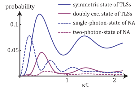
Fig. 4: Probabilities of different atomic and nanoantenna excitations vs. normalized time. Strong coupling between the atomic systems and the nanoantenna is manifested in the dynamics by the mutual exchange of excitations (atomic - solid lines, nanoantenna - dashed lines). Peaks in occupation probabilities of the symmetric (blue solid line, results multiplied by a factor of $0.5$) and doubly excited (purple solid line) states, correspond to dips in probabilities of the presence of one (blue dashed line) and two (purple dashed line) photons in the system. Nanoantenna and atomic parameters are described in the text.

V Modification of Spectra

In this section we shall study how the presence of two atoms coupled to a nanoantenna modifies its extinction spectrum. Such modification is profound for strong coupling and in the quantum regime. In this work we may refer to the quantum regime as a situation, where the mean number of excitations in the system is at the single-quantum level. We compare the results with the single atom case to prove the sensitivity of the hybrid quantum system to the number of atomic systems involved.

The hybrid system permits several loss channels, namely radiative and non-radiative losses of the nanoantenna and the spontaneous emission and dephasing in the atomic density matrix. The total extinct (absorbed and scattered) power is given by

$$P(\omega_{\mathrm{dr}})\equiv\hbar\omega_{\mathrm{na}}\Gamma\langle a^{\dagger}a\rangle+\sum_{j}^{N_{\mathrm{tls}}}\hbar\omega_{0}\Gamma_{\mathrm{fs}}\langle\sigma_{+}^{\left(j\right)}\sigma_{-}^{\left(j\right)}\rangle\ \ ,$$

containing the contributions from the nanoantenna and the atoms, respectively. This quantity is directly accessible in a potential experiment. Here, $\langle a^{\dagger}a\rangle=\mathrm{Tr}\left[a^{\dagger}a\rho(t\rightarrow\infty)\right]$ denotes the mean number of photons in the system’s steady state $\rho(t\rightarrow\infty)$. Similarly, $\langle\sigma_{+}^{\left(j\right)}\sigma_{-}^{\left(j\right)}\rangle$ corresponds to the excited-state occupation probability of the $j^{\mathrm{th}}$ atom.

In the present study the loss rate of the nanoantenna is much larger than that of the bare atoms, $\Gamma\gg\Gamma_{\mathrm{fs}}$, see again Sec. IV. Thus, the loss of the nanoantenna can be used as a an extremely good approximation of the loss of the hybrid system Chang et al. (2006).

The spectra are calculated using a freely available quantum optics toolbox Tan (1999). Note that because of the rather low efficiency of the nanoantenna, i.e. $\Gamma_{\mathrm{nr}}\gg\Gamma_{\mathrm{r}}$, the extinction spectrum is dominated by the absorption spectrum.

Even though the losses are almost entirely due to the nanoantenna, the extinction spectrum may be strongly influenced by the two atoms. In particular, this is the case when the driving field is weak and the hybrid system remains at the single-excitation level, i.e. in the quantum regime. This large atomic contribution to the overall spectrum naturally depends significantly on the coupling as it is illustrated in Fig. 5. For weak coupling [see panel (a)], a broad resonance of the nanoantenna dominates the extinction spectrum and a perturbation at the transition frequency of the atoms can be observed. For strong coupling [panel (b)], the plasmonic and atomic contributions to the spectrum can no longer be distinguished. The extinction at the atomic transition frequency gets significantly reduced and Rabi peaks are visible at the sides. Due to the strong coupling the spectral shift of the extinction peaks can be significantly exceed the linewidth. Thus strong coupling evokes a large effect of the atoms on the extinction spectrum of the nanoantenna.

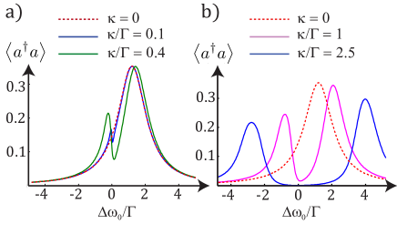
Fig. 5: Impact of atoms on the extinction spectra of the hybrid system for different coupling strengths $\kappa$ in the weak (a) and strong coupling regime (b). The steady-state mean number of photons is plotted vs. the driving-field normalized detuning from the atomic transition frequency $\Delta\omega_{0}/\Gamma$. For the sake of comparison the spectrum of the bare nanoantenna (no coupling, $\kappa=0$) has been added. A Fano-like behavior can be observed for increased but still weak coupling. The results have been obtained for a weak driving field (Rabi frequency $\Omega=0.6\Gamma$). Furthermore, a rather small detuning between nanoantenna resonance and atomic transition frequency ($\omega_{\mathrm{na}}-\omega_{0}=1.2\Gamma$) has been assumed. The blue line in panel (b) corresponds to the antenna design of Sec. IV.

Generally, the spectrum can be understood in terms of hybridization caused by the interaction of all sub-systems Meystre and Sargent (1999). The eigenstates and eigenenergies can be derived on the basis of the Jaynes-Cummings model which is outlined in App. C in detail. The eigenenergies are plotted in Fig. 6 for the cases of a single and two atoms coupled to the nanoantenna. In the resonant case ($\omega_{\mathrm{na}}=\omega_{0}$) the splitting between the first pair of excited eigenstates is equal to $\sqrt{N_{\mathrm{tls}}}\kappa$. This simple example proves that the spectrum of the hybrid system, i.e. the position of the Rabi peaks, crucially depends on the number of atoms. Furthermore, the effective increase of the coupling constant by the factor of $\sqrt{N_{\mathrm{tls}}}$ may help to overcome losses and fulfill the strong coupling condition (18).

The analysis of the diagrams in Fig. 6 suggests that, in principle, one might expect an even stronger manifestation of the number of atoms in the spectra for slightly more intense driving fields, where highly-excited states ($n\geq 2$) become occupied. For this purpose, however, a coupling even stronger than that obtained with the design of Sec. IV would be preferable. Otherwise, due to significant nanoantenna losses the required sensitivity to trace the contribution of highly excited states to the spectra cannot be reached.

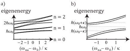
Fig. 6: (a) Eigenenergies of the hybrid system as function of the detuning between nanoantenna resonance and atomic transition frequency for the case of $N_{\mathrm{tls}}=1$ (dashed lines) and $N_{\mathrm{tls}}=2$ (solid lines). Only energies of states corresponding to the total number of excitations $n\leq 2$ are shown. (b) Zoomed view for $n=1$. Energy splitting of the first pair of excited states compared for the cases $N_{\mathrm{tls}}=1$ and $N_{\mathrm{tls}}=2$. In the latter case it is larger by a factor of $\sqrt{2}$ for $\omega_{\mathrm{na}}=\omega_{0}$.

The interesting question arises whether the influence of the atoms on the extinction spectra remains so significant for stronger driving fields, i.e. beyond the quantum regime. To investigate such transition we performed calculations for increasing driving intensities for the strong-coupling design proposed in Section IV. The results are displayed in Fig. 7(a). For weak driving fields (blue line) a splitting can be observed with Rabi peaks at $\Delta\omega_{0}=\pm\sqrt{2}\kappa$ as well as an onset of transparency at $\Delta\omega_{0}=0$, as measured in cavity QED systems, see Refs. Hood et al. (1998); Miller et al. (2005). For stronger driving fields the corresponding extinction peaks are shifted towards the center. Finally, in the limit of a strong driving field ($\Omega>\Gamma$), the contribution from the atomic system becomes negligible and the bare nanoantenna spectrum is recovered.

To understand this behavior, we analyze the occupation probabilities of the hybrid system’s eigenstates. For weak driving fields only the first pair of excited eigenstates $|\psi_{1,\pm}\rangle$ with energies equal to $\hbar\omega_{0}\pm\hbar\sqrt{2}\kappa$ is populated. For this case the occupation probabilities of the states $|\psi_{1,+}\rangle$ and $|\psi_{2,+}\rangle$ are plotted in Fig. 7(b). It can be seen that for the latter state it is indeed negligible. The occupation probabilities of states $|\psi_{1,-}\rangle$ and $|\psi_{2,-}\rangle$ (not shown) are peaks symmetric with respect to $|\psi_{1,+}\rangle$ and $|\psi_{2,+}\rangle$, i.e. they are centered at $\omega=\omega_{0}+\sqrt{2}\kappa$. For an increased driving field, the probability of exciting higher-energy states becomes significant [see green lines in Fig. 7(b)]. This is the reason for the shift of the Rabi peaks Meystre and Sargent (1999) towards the center. If the driving field rises, the energy difference between subsequent occupied eigenstates converges towards $\omega_{\mathrm{na}}$, which explains why in the strong driving field limit ($\Omega>\Gamma$) the result corresponds to the bare nanoantenna case. This result can also be derived from the steady-state solution of the Heisenberg equations of motion where one finds that $\langle a^{\dagger}a\rangle\approx\Omega^{2}/\Gamma^{2}\gg N_{\mathrm{tls}}$ holds. This means that indeed for stronger driving fields the classical behavior of the nanoantenna is re-established, irrespective of the presence of the atoms.

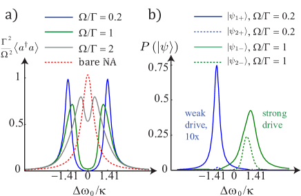
Fig. 7: (a) Impact of the driving field intensity on the extinction spectra, normalized by a dimensionless parameter $\Omega^{2}/\Gamma^{2}$, for the strongly coupled nanoantenna proposed in Sec. IV. (b) Probability of occupation of the first ($n=1$, solid lines) and second ($n=2$, dashed lines) pair of excited states $|\psi_{n,\pm}\rangle$ for a driving field with Rabi frequencies $\Omega=0.2\Gamma$ (blue lines, results multiplied by a factor of $10$) and $\Omega=\Gamma$ (green lines).

VI Conclusions

In this paper, we have investigated the coupling of one and two atoms approximated by two-level systems to optical nanoantennas. It was outlined that a full quantum approach is required to understand the dynamics of the hybrid system. Only for extremely weak driving fields a semiclassical formulation of the nanoantenna dynamics may be used.

At the design stage for a nanoantenna a trade-off must be taken into account between the field enhancement by the nanoantenna, directly responsible for the strength of the coupling, and the nanoantenna’s efficiency. Small size, which results in high absorption losses, is essential for achieving the strong coupling regime. Then, the spectra of the hybrid system are hugely influenced by the presence of the atoms provided that the driving field is considerably weak, i.e. in the quantum regime.

Furthermore we have shown that a strong coupling of several atoms to a nanoantenna does change the spectrum significantly. Such features will enable experimentalists to identify situations of multiple coupled atoms in the strong coupling regime.

Appendix A The dynamics of the classical field

In this section we will outline the semiclassical treatment of the nanoantenna used in this paper. Especially, we will derive the equations of motion for the respective electric field in dependence on the state of the atoms.

If a plasmonic structure like the discussed nanoantenna is much smaller than the wavelength, it can be treated as a classical harmonic oscillator as well-known in the metamaterials community, see e.g. Ref. Petschulat et al. (2008). The scattered field $\tilde{\mathbf{E}}_{\mathrm{exc}}\left(\mathbf{r},t\right)$ of such an oscillator may be separated into temporally and spatially varying contributions:

$$\tilde{\mathbf{E}}_{\mathrm{exc}}\left(\mathbf{r},t\right) = \tilde{\alpha}\left(t\right)\mathbf{E}_{\mathrm{exc}}\left(\mathbf{r}\right)+\mathrm{c.c.}\ ,$$ (19)

where the subscript ’exc’ is used to label the excited field of the nanoantenna. This notation renders it unnecessary to distinguish between the scattered field of the nanoantenna and the field inside its metallic body. The spatial part $\mathbf{E}_{\mathrm{exc}}\left(\mathbf{r}\right)$ can be found by computer simulations or analytical considerations. By definition we assume that this spatial contribution, which may also be denoted as mode profile, does not change with time for the excitations we discuss in the following. Then, the whole nanoantenna dynamics is exclusively described by the evolution of the temporal part $\tilde{\alpha}\left(t\right)$ for which the equations of motion will be derived and solved in the following.

Under the assumption of an oscillator-like evolution, the positive frequency part $\tilde{\alpha}\left(t\right)$ evolves according to the equation

$$\ddot{\tilde{\alpha}}\left(t\right)+\Gamma\dot{\tilde{\alpha}}\left(t\right)+\omega_{\mathrm{na}}^{2}\tilde{\alpha}\left(t\right) = F\left(t\right)e^{-i\omega_{\mathrm{dr}}t},$$ (20)

where $F\left(t\right)e^{-i\omega_{\mathrm{dr}}t}$ is the driving field at the nanoantenna’s site. In our case it is proportional to the driving laser field and the assumed dipolar fields of the two atoms.

We assume the driving term to oscillate at the mean frequency $\omega_{\mathrm{dr}}$. Then, its envelope $F\left(t\right)$ varies much slower. Consequentially, we can also calculate the solutions to the equations of motion for the slowly-varying part of the nanoantennas oscillation defined via $\tilde{\alpha}\left(t\right)=\alpha\left(t\right)e^{-i\omega_{\mathrm{dr}}t}$. Then using the standard slowly-varying envelope approximation ( $\left|\dot{\alpha}\right|\ll\left|\alpha\omega_{\mathrm{dr}}\right|$) and accounting for $\Gamma\ll\omega_{\mathrm{dr}}$ one arrives at the equations of motion for the electric field of the nanoantenna as

$$\dot{\alpha}\left(t\right)=-\Gamma\alpha\left(t\right)+\frac{i}{2\omega_{\mathrm{dr}}}\left[\left(\omega_{\mathrm{dr}}^{2}-\omega_{\mathrm{na}}^{2}\right)\alpha(t)+F\left(t\right)\right].$$ (21)

For near-resonance driving fields ($\omega_{\mathrm{na}}^{2}-\omega_{\mathrm{dr}}^{2}\approx 2\omega_{\mathrm{dr}}\Delta\omega_{\mathrm{na}}$), the above equation further reduces to:

$$\dot{\alpha}\left(t\right)=-\left(\Gamma+i\Delta\omega_{\mathrm{na}}\right)\alpha\left(t\right)+iF\left(t\right)/2\omega_{\mathrm{dr}}\ ,$$ (22)

We now compare equation (22) with the Heisenberg operator equation in the fully quantum approach, $\dot{a}\left(t\right)=-\left(\Gamma+i\Delta\omega_{\mathrm{na}}\right)a\left(t\right)+i\left[\kappa\sum_{j}\sigma_{-}^{(j)}\left(t\right)+\Omega\right]+f(t)$, where $f(t)$ stands for the Langevin noise operator such that $\langle f(t)\rangle=0$ Meystre and Sargent (1999), which origins from coupling of the field of the nanoantenna with its electromagnetic environment and with phonons. With such a direct comparison, we can identify the driving term

$$F\left(t\right) = 2\omega_{\mathrm{dr}}\left[\kappa\sum_{j}{\rho_{eg}^{\mathrm{sc}}}^{(j)}(t)+\Omega\right]\ ,\ \mathrm{so}$$ (23)

and get eventually

$$\dot{\alpha}\left(t\right)=-\left(\Gamma+i\Delta\omega_{\mathrm{na}}\right)\alpha\left(t\right)+i\left[\kappa\sum_{j}{\rho_{eg}^{\mathrm{sc}}}^{(j)}(t)+\Omega\right]$$ (24)

as the evolution equation for the electric field of the nanoantenna in the semiclassical approximation. Our result corresponds to the equation of motion of the expectation value of quantum operators if the nanoantenna’s field is approximated by a coherent state $|\alpha\left(t\right)\rangle$.

Appendix B Calculation of parameters

In Appendix A we have derived the equations of motion for the electric field of a nanoantenna coupled to an unspecified number of noninteracting atoms. Now we will specify how to obtain the relevant system parameters from electromagnetic simulations. The key for determining the coupling constants and loss rates lies in the determination of the nanoantenna field for a single excitation as we will see shortly.

Coupling constant between
nanoantenna and atoms: $\kappa$

In electric dipole approximation the parameter $\kappa$ describing the coupling strength between the $j^{\mathrm{th}}$ atom and the nanoantenna is given by

$$\kappa_{j}=\mathbf{E}_{\mathrm{exc}}^{\mathrm{se}}\left(\mathbf{r}_{j}\right)\cdot\mathbf{d}_{ge}^{(j)}/\hbar\ ,$$ (25)

where $\mathbf{d}_{ge}^{(j)}$ stands for the transition dipole moment in the $j^{\mathrm{th}}$ atom positioned at $\mathbf{r}_{j}$. In the considered case the atoms are assumed to be identical, so the index $j$ can be dropped. Naturally, here the field $\mathbf{E}_{\mathrm{exc}}^{\mathrm{se}}$ corresponds to a single excitation of the nanoantenna subject to a plane-wave excitation. Because of the atomic system’s symmetric positioning and the mirror-symmetry of the nanoantenna, $\mathbf{E}_{\mathrm{exc}}^{\mathrm{se}}\left(\mathbf{r}_{1}\right)=\mathbf{E}_{\mathrm{exc}}^{\mathrm{se}}\left(\mathbf{r}_{2}\right)$ the excitation of the antisymmetric state of the atomic system for the lossless case is prohibited, see App. C. It is evident that $\kappa$ depends on the dipole moment of both atoms, the electric field of the nanoantenna’s mode and the very location of the atoms. Obviously, this scheme of calculating the field of the nanoantenna corresponds to a dipolar mode approximation since the plane wave mainly couples to the dipolar mode of the nanoantenna. Higher order contributions are neglectedYan et al. (2008), which has two consequences: the coupling strengths $\kappa_{j}$ as well as the nonradiative loss rate of the nanoantenna, $\Gamma_{\mathrm{nr}}$, are underestimated. We have chosen to restrict our investigations to this simplified scheme as the inclusion of higher order nanoantenna modes significantly complicates the analysis of the system dynamics and also prevents us from finding accessible analytical results.

To find the correct scaling for $\kappa$, the electric field has to be calculated at the positions of the atoms for an excitation of the nanoantenna by a single photon with energy $\hbar\omega_{\mathrm{na}}$. Thus, for the computation at the nanoantenna’s resonance, first the field energy for the corresponding excited electromagnetic mode $\mathbf{E}_{\mathrm{exc}}\left(\mathbf{r}\right)$ has to be determined using the well-known energy-density integration for dispersive media Landau et al. (1982)

$$W = \frac{1}{2}\int\left.\frac{\partial}{\partial\omega}\left[\omega\,\Re\varepsilon\left(\omega\right)\right]\right|_{\omega=\omega_{\mathrm{na}}}\left|E_{\mathrm{exc}}\left(\mathbf{r}\right)\right|^{2}dV$$

$$+\frac{1}{2}\int\mu_{0}\left|H_{\mathrm{exc}}\left(\mathbf{r}\right)\right|^{2}dV\ .$$

Then, the electric field of a single-photon excitation is given by

$$\mathbf{E}_{\mathrm{exc}}^{\mathrm{se}}\left(\mathbf{r}\right) = \sqrt{\hbar\omega_{\mathrm{na}}/W}\,\mathbf{E}_{\mathrm{exc}}\left(\mathbf{r}\right)\ ,$$ (27)

since the energy of the nanoantenna’s mode corresponds to $N=W/\hbar\omega_{\mathrm{na}}$ photons.

Coupling constant between nanoantenna
and driving field: Rabi frequency $\Omega$

The Rabi frequency $\Omega$ describes the coupling of the nanoantenna and the driving field. It can be evaluated in the dipole approximation as $\Omega=\mathbf{d}_{\mathrm{na}}^{\mathrm{se}}\cdot\mathbf{E}_{\mathrm{dr}}/\hbar$, where $\mathbf{d}_{\mathrm{na}}^{\mathrm{se}}$ is the dipole moment of the nanoantenna corresponding to a single excitation for which the electric field is known from the previous subsection. The dipole moment $\mathbf{d}_{\mathrm{na}}^{\mathrm{se}}$ can then just be calculated from a multipole expansion of $\mathbf{E}_{\mathrm{exc}}^{\mathrm{se}}\left(\mathbf{r}\right)$. For our calculations, the main contribution to the far-field of the nanoantenna was indeed that from the dipole moment which justifies the calculation of $\Omega$ in the dipole approximation.

Radiative and nonraditive losses
of the nanoantenna: $\Gamma$

The losses of the nanoantenna can be divided into radiative and non-radiative losses, $\Gamma=\Gamma_{\mathrm{r}}+\Gamma_{\mathrm{nr}}$. Both quantities are related to integrations of the nanoantenna mode for a single excitation $\mathbf{E}_{\mathrm{exc}}^{\mathrm{se}}\left(\mathbf{r}\right)$: The radiative loss $\Gamma_{\mathrm{r}}$ can be determined by integrating the time-averaged Poynting vector over a closed surface embedding the nanoantenna, $\Gamma_{\mathrm{r}}=\int\left\langle\mathbf{S}_{\mathrm{exc}}^{\mathrm{se}}\left(\mathbf{r},t\right)\right\rangle d\mathbf{A}$. The non-radiative part is given by a volume integral over the nanoantenna using Ohm’s law, $\Gamma_{\mathrm{nr}}=\int\sigma\left\langle\mathbf{E}_{\mathrm{exc}}^{\mathrm{se}}\left(\mathbf{r},t\right)\right\rangle^{2}dV$, where $\sigma$ is the electric conductivity of the metal.

Appendix C Eigenstates of the free Hamiltonian

Now we are going to analyze the Hamiltonian of the nanoantenna coupled to two two-level systems in the fully quantum case. As one might expect, we will arrive at a simple generalization of the Jaynes-Cummings model and give the energy spectrum of the hybrid system’s eigenstates.

It is often advantageous to analyze problems of coupled two-level systems in the so-called Dicke basis that relates ground and excited states, $|g\rangle$ and $|e\rangle$, of each two-level system to a combined eigenbasis Dicke (1954): $\left\{|D\rangle\equiv|e\rangle\otimes|e\rangle\right.$, $|S\rangle\equiv\frac{1}{\sqrt{2}}\left(|e\rangle\otimes|g\rangle+|g\rangle\otimes|e\rangle\right)$, $|A\rangle\equiv\frac{1}{\sqrt{2}}\left(-|e\rangle\otimes|g\rangle+|g\rangle\otimes|e\rangle\right)$, $\left.|G\rangle\equiv|g\rangle\otimes|g\rangle\right\}$, with the doubly excited state $|D\rangle$, the symmetric and antisymmetric states $|S\rangle$ and $|A\rangle$ with a single excitation, and the ground state $|G\rangle$. In the Dicke basis, the Hamiltonian reads as

$$H = \frac{1}{2}\hbar\omega_{0}\left(2|D\rangle\langle D|+|S\rangle\langle S|+|A\rangle\langle A|\right)+\hbar\omega_{\mathrm{na}}a^{\dagger}a$$ (28)

$$-\hbar\sqrt{2}\kappa\left(\Sigma_{+}a+a^{\dagger}\Sigma_{-}\right)\ ,$$

where

$$\Sigma_{+} = \frac{1}{\sqrt{2}}\left(\sigma_{+}^{(1)}+\sigma_{+}^{(2)}\right)=|D\rangle\langle S|+|S\rangle\langle G|\ \mathrm{and}$$

$$\Sigma_{-} = \Sigma_{+}^{\dagger},$$

are the creation and annihilation operators of an excitation in the atomic subsystem. Note that the antisymmetric state is decoupled in the isolated system and can be populated only by decay mechanisms or by an asymmetric drive. From now on it suffices to consider only the effective three-level system, whose state belongs to the Hilbert space spanned by $\{|G\rangle,|S\rangle,|D\rangle\}$.

We will give the explicit form of the eigenstates of the Hamiltonian and the corresponding eigenenergies in the case of resonance between the atomic and plasmonic systems, i.e. when $\omega_{\mathrm{na}}=\omega_{0}$. The states of the hybrid system can be expressed in the Dicke basis for the atomic subsystem, and in the Fock basis $\{|k\rangle\}_{k=0}^{\infty}$ for the nanoantenna, with $k$ denoting the number of photons in the system.

Each state can be characterized by the total number of excitations $n$ it corresponds to. For instance, $n=0$ stands for the total ground state of the system $|\psi_{0}\rangle=|G,0\rangle$ of energy $E_{0}=0$. For a single excitation $n=1$ we have two eigenstates and eigenvalues:

$$|\psi_{1,\pm}\rangle = \pm|S,0\rangle+|G,1\rangle,$$ (29)

$$E_{1,\pm} = \hbar\omega_{0}\mp\sqrt{2}\hbar\kappa.$$ (30)

For the numbers of excitations $n\geq 2$ there are three eigenstates for a given $n$:

$$|\psi_{n,\pm}\rangle = \sqrt{n-1}|D,n-2\rangle$$

$$\pm\sqrt{2n-1}|S,n-1\rangle+\sqrt{n}|G,n\rangle,$$

$$E_{n,\pm} = n\hbar\omega_{0}\mp\sqrt{2\left(2n-1\right)}\hbar\kappa,$$ (32)

$$|\psi_{n,0}\rangle = \sqrt{n}|D,n-2\rangle-\sqrt{n-1}|G,n\rangle,$$ (33)

$$E_{n,0} = n\hbar\omega_{0}.$$ (34)

For visibility, the states are not normalized. Note that the eigenstates of the total system cannot be written as a product of states of atomic and nanoantenna subsystems. This is a clear sign of strong interaction of the subsystems that leads to their entanglement. The latter is a sole quantum feature which cannot be accounted for with the semiclassical formalism. Our condition for the validity of the semiclassical approach can now be seen from a different perspective: the semiclassical description can be applied only if entanglement is present in the system with negligible probability.

The eigenstates attain a more complicated form, if the two-level systems are not in resonance with the nanoantenna ($\omega_{\mathrm{na}}\neq\omega_{0}$). Then, the energy diagram depends strongly on the detuning, see again Fig. 6. In the strongly off-resonant limit, the interaction becomes negligible and the atomic and the nanoantenna subsystems behave independently. Consequentially, the eigenenergies converge towards the unperturbed values.

For large numbers of excitations, the eigenstates become approximately separable:

$$|\psi_{n,\pm}\rangle \approx \left(|D\rangle\pm\sqrt{2}|S\rangle+|G\rangle\right)\otimes|n\rangle,$$ (35)

$$|\psi_{n,0}\rangle \approx \left(|D\rangle-|G\rangle\right)\otimes|n\rangle,$$ (36)

with the interaction energies: $\Delta E_{n,\pm}=\mp 2\hbar\kappa\sqrt{n}$, $\Delta E_{n,0}=0$. This means, that in the limit of large field intensities, even though the field has strong influence on the atoms, the atoms approximately do not affect the field and the semiclassical approach can be applied again.

References

- Anger et al. (2006) P. Anger, P. Bharadwaj, and L. Novotny, Phys. Rev. Lett. 96, 113002 (2006).
- Pfeiffer et al. (2010) M. Pfeiffer, K. Lindfors, C. Wolpert, P. Atkinson, M. Benyoucef, A. Rastelli, O. G. Schmidt, H. Giessen, and M. Lippitz, Nano Letters 10, 4555 (2010).
- Curto et al. (2010) A. G. Curto, G. Volpe, T. H. Taminiau, M. P. Kreuzer, R. Quidant, and N. F. van Hulst, Science 329, 930 (2010).
- Zhu et al. (2012) X. Zhu, F. Xie, L. Shi, X. Liu, N. A. Mortensen, S. Xiao, J. Zi, and W. Choy, Opt. Lett. 37, 2037 (2012).
- Filter et al. (2013) R. Filter, M. Farhat, M. Steglich, R. Alaee, C. Rockstuhl, and F. Lederer, Optics Express 21, 3737 (2013).
- Mohtashami and Koenderink (2013) A. Mohtashami and A. F. Koenderink, New J. Phys. 15, 043017 (2013).
- Novotny and van Hulst (2011) L. Novotny and N. van Hulst, Nat. Phot. 5, 83 (2011).
- Rogobete et al. (2007) L. Rogobete, F. Kaminski, M. Agio, and V. Sandoghdar, Opt. Lett. 32, 1623 (2007).
- Kern et al. (2012) J. Kern, S. Grossmann, N. V. Tarakina, T. Häckel, M. Emmerling, M. Kamp, J.-S. Huang, P. Biagioni, J. C. Prangsma, and B. Hecht, Nano Lett. 12, 5504 (2012).
- Kern and Martin (2012) A. M. Kern and O. J. F. Martin, Phys. Rev. A 85, 022501 (2012).
- Filter et al. (2012) R. Filter, S. Mühlig, T. Eichelkraut, C. Rockstuhl, and F. Lederer, Phys. Rev. B 86, 035404 (2012).
- Yoshie et al. (2004) T. Yoshie, A. Scherer, J. Hendrickson, G. Khitrova, H. M. Gibbs, G. Rupper, C. Ell, O. B. Shchekin, and D. G. Deppe, Nature 432, 200 (2004).
- Reithmaier et al. (2004) J. P. Reithmaier, G. Sęk, A. Löffler, C. Hofmann, S. Kuhn, S. Reitzenstein, L. V. Keldysh, V. D. Kulakovskii, T. L. Reinecke, and A. Forchel, Nature 432, 197 (2004).
- Aoki et al. (2006) T. Aoki, B. Dayan, E. Wilcut, W. Bowen, A. Parkins, T. J. Kippenberg, K. J. Vahala, and H. J. Kimble, Nature 443, 671 (2006).
- Yan et al. (2008) J. Y. Yan, W. Zhang, S. Duan, X. G. Zhao, and A. O. Govorov, Phys. Rev. B 77, 165301 (2008).
- Artuso et al. (2011) R. D. Artuso, G. W. Bryant, A. Garcia-Etxarri, and J. Aizpurua, Phys. Rev. B 83, 235406 (2011).
- Meystre and Sargent (1999) P. Meystre and M. Sargent, Elements of Quantum Optics (Springer Verlag, 1999).
- Zuloaga et al. (2010) J. Zuloaga, E. Prodan, and P. Nordlander, ACS Nano 4, 5269 (2010).
- Manjavacas et al. (2011) A. Manjavacas, F. J. Garcia de Abajo, and P. Nordlander, Nano Lett. 11, 2318 (2011).
- Trügler and Hohenester (2008) A. Trügler and U. Hohenester, Phys. Rev. B 77, 115403 (2008).
- Waks and Sridharan (2010) E. Waks and D. Sridharan, Phys. Rev. A 82, 043845 (2010).
- Dzsotjan et al. (2011) D. Dzsotjan, J. Kästel, and M. Fleischhauer, Phys. Rev. B 84, 075419 (2011).
- Zhang and Govorov (2011) W. Zhang and A. O. Govorov, Phys. Rev. B 84, 081405 (2011).
- Hümmer et al. (2013) T. Hümmer, F. J. Garcia-Vidal, L. Martin-Moreno, and D. Zueco, Phys. Rev. B 87, 115419 (2013).
- Wolters et al. (2012) J. Wolters, G. Kewes, A. W. Schell, N. Nüsse, M. Schoengen, B. Löchel, T. Hanke, R. Bratschitsch, A. Leitenstorfer, T. Aichele, et al., Phys. Status Solidi B 249, 918 (2012).
- Słowik et al. (2012) K. Słowik, A. Raczyński, J. Zaremba, and S. Zielińska-Kaniasty, Optics Communications 285, 2392 (2012).
- Lembessis and Babiker (2013) V. E. Lembessis and M. Babiker, Phys. Rev. Lett. 110, 083002 (2013).
- Heiss et al. (2007) D. Heiss, S. Schaeck, H. Huebl, M. Bichler, G. Abstreiter, J. J. Finley, D. V. Bulaev, and D. Loss, Phys. Rev. B 76, 241306 (2007).
- Chen et al. (2013) X.-W. Chen, V. Sandoghdar, and M. Agio, Phys. Rev. Lett. 110, 153605 (2013).
- Dorner and Zoller (2002) U. Dorner and P. Zoller, Phys. Rev. A 66, 023816 (2002).
- Wolfram (1999) S. Wolfram, The MATHEMATICA Book, Version 4 (Cambr. Univ. Pr., 1999).
- Wallraff et al. (2004) A. Wallraff, D. I. Schuster, A. Blais, L. Frunzio, R.-S. Huang, J. Majer, S. Kumar, S. M. Girvin, and R. J. Schoelkopf, Nature 431, 162 (2004).
- Andreani et al. (1999) L. C. Andreani, G. Panzarini, and J.-M. Gérard, Phys. Rev. B 60, 13276 (1999).
- Savasta et al. (2010) S. Savasta, R. Saija, A. Ridolfo, O. Di Stefano, P. Denti, and F. Borghese, ACS Nano 4, 6369 (2010).
- Novotny and Hecht (2006) L. Novotny and B. Hecht, Principles Of Nano-Optics (Cambridge University Press, 2006).
- Bharadwaj et al. (2009) P. Bharadwaj, B. Deutsch, and L. Novotny, Adv. Opt. Photon. 1, 438 (2009).
- Palik (1985) E. D. Palik, Handbook of Optical Constants of Solids, no. Bd. 1 in Handbook of Optical Constants of Solids, Five-Volume Set (Elsevier Science, 1985).
- Ge et al. (2013) R.-C. Ge, C. Van Vlack, P. Yao, J. F. Young, and S. Hughes, Phys. Rev. B 87, 205425 (2013).
- Mu and Savage (1992) Y. Mu and C. M. Savage, Phys. Rev. A 46, 5944 (1992).
- Maksymov et al. (2012) I. S. Maksymov, A. E. Miroshnichenko, and Y. S. Kivshar, Phys. Rev. A 86, 011801 (2012).
- Bohren and Huffman (1998) C. Bohren and D. R. Huffman, Absorption and Scattering of Light by Small Particles (Wiley Science Paperback Series, 1998).
- Gonzalez-Tudela et al. (2011) A. Gonzalez-Tudela, D. Martin-Cano, E. Moreno, L. Martin-Moreno, C. Tejedor, and F. J. Garcia-Vidal, Phys. Rev. Lett. 106, 020501 (2011).
- Martin-Cano et al. (2011) D. Martin-Cano, A. González-Tudela, L. Martin-Moreno, F. J. Garcia-Vidal, C. Tejedor, and E. Moreno, Phys. Rev. B 84, 235306 (2011).
- Sidorkin et al. (2009) V. Sidorkin, E. van Veldhoven, E. van der Drift, P. Alkemade, H. Salemink, and D. Maas, J. Vac. Sci. Technol. B: Microelectronics and Nanometer Structures 27, L18 (2009).
- Bleuse et al. (2011) J. Bleuse, J. Claudon, M. Creasey, N. S. Malik, J.-M. Gérard, I. Maksymov, J.-P. Hugonin, and P. Lalanne, Phys. Rev. Lett. 106, 103601 (2011).
- Chen et al. (2012) I.-H. Chen, K.-H. Chen, W.-T. Lai, and P.-W. Li, IEEE Transactions on Electron Devices 59, 3224 (2012).
- Alaee et al. (2013) R. Alaee, C. Menzel, U. Huebner, E. Pshenay-Severin, S. Bin Hasan, T. Pertsch, C. Rockstuhl, and F. Lederer, Nano Lett. 13, 3482 (2013).
- Chang et al. (2006) D. E. Chang, A. S. Sørensen, P. R. Hemmer, and M. D. Lukin, Phys. Rev. Lett. 97, 053002 (2006).
- Tan (1999) S. M. Tan, J. Opt. B 1, 424 (1999).
- Hood et al. (1998) C. J. Hood, M. S. Chapman, T. W. Lynn, and H. J. Kimble, Phys. Rev. Lett. 80, 4157 (1998).
- Miller et al. (2005) R. Miller, T. E. Northup, K. M. Birnbaum, A. Boca, A. D. Boozer, and H. J. Kimble, J. Phys. B: At. Mol. Opt. Phys. 38, S551 (2005).
- Petschulat et al. (2008) J. Petschulat, C. Menzel, A. Chipouline, C. Rockstuhl, A. Tuennermann, F. Lederer, and T. Pertsch, Phys. Rev. A 78, 043811 (2008).
- Landau et al. (1982) L. D. Landau, E. M. Lifshitz, and L. P. Pitaevskii, Electrodynamics of Continous Media; Landau and Lifshitz Course of Theoretical Physics, vol. 2nd (Butterworth-Heinenann, Boston, MA, 1982).
- Dicke (1954) R. H. Dicke, Phys. Rev. 93, 99 (1954).