Shape evolution of giant resonances in Nd and Sm isotopes

Abstract

Giant multipole resonances in Nd and Sm isotopes are studied by employing the quasiparticle-random-phase approximation on the basis of the Skyrme energy-density-functional method. Deformation effects on giant resonances are investigated in these isotopes which manifest a typical nuclear shape change from spherical to prolate shapes. The peak energy, the broadening, and the deformation splitting of the isoscalar giant monopole (ISGMR) and quadrupole (ISGQR) resonances agree well with measurements. The magnitude of the peak splitting and the fraction of the energy-weighted strength in the lower peak of the ISGMR reflect the nuclear deformation. The experimental data on ISGMR, ISGDR, and ISGQR are consistent with the nuclear-matter incompressibility $K\simeq 210-230$ MeV and the effective mass $m^{*}_{0}/m\simeq 0.8-0.9$. However, the high-energy octupole resonance (HEOR) in ¹⁴⁴Sm seems to indicates a smaller effective mass, $m^{*}_{0}/m\simeq 0.7-0.8$. A further precise measurement of HEOR is desired to determine the effective mass.

I Introduction

Giant resonance (GR) is a typical high-frequency collective mode of excitation in nuclei har01 . Effects of the nuclear deformation on the GRs have been investigated both experimentally and theoretically. Among them, the deformation splitting of the isovector giant dipole resonance (GDR), due to different frequencies of oscillations along the major- and minor-axis BM2 , is well established. A textbook example of the evolution of the GDR as a function of the mass number can be foundin Refs. car71 ; car74 . Emergence of a double-peak structure of the photoabsorption cross section of ¹⁵⁰Nd and ¹⁵²Sm clearly indicates an onset of the deformation in the ground state. For the GRs with higher multipolarity, although the deformation splitting is less pronounced, the peak broadening has been observed har01 . The detailed and systematic investigations on the GRs would give us a unique information on the shape phase transition in nuclei.

In contrast to low-energy modes of excitation in nuclei, the GRs substantially reflect bulk nuclear properties. Thus, their studies may provide information on the nuclear matter. The GRs can be qualitatively investigated by using various macroscopic models, such as fluiddynamical models which properly take account of deformation of the Fermi sphere RS . However, a quantitative description of the GRs requires a microscopic treatment of nuclear response. For heavy deformed open-shell nuclei, the leading theory for this purpose is, currently, the quasiparticle-random-phase approximation (QRPA) based on the nuclear energy-density-functional (EDF) method ben03 . The QRPA based on the deformed ground-state configuration with superfluidity is able to treat a variety of excitations in the linear regime. A role of deformation on GRs has been studied by means of the deformed QRPA employing the Gogny interaction in the light mass region per08 . GRs in heavy systems have been investigated using Skyrme functionals, where the separable approximation is employed for the residual interaction nes06 , and using the relativistic EDF pen09 .

The Hartree-Fock-Bogoliubov (HFB) mean field formulated in the two-dimensional cylindrical coordinates and the deformed QRPA in the quasiparticle basis have been developed recently yos08 . The application, however, was restricted to light systems yos09a because of the large computer memory demanded for storing the matrix elements, and the time-consuming calculation for diagonalizing a non-symmetric matrix of several tens or hundreds of thousands of dimensions. The deformed Skyrme-QRPA calculation utilizing the transformed harmonic oscillator basis is also restricted to light nuclei due to the same stumbling block los10 . Recently, the finite amplitude method nak07 ; avo11 is applied to the harmonic-oscillator-basis deformed QRPA and the calculation for heavy systems becomes possible with an inexpensive numerical cost sto11 , while it is restricted to the $K^{\pi}=0^{+}$ mode so far.

In this article, we develop a new calculation code of the deformed HFB and QRPA for use in the massively parallel computers to examine the applicability of the Skyrme-EDF-based QRPA to the excitation modes in heavy deformed systems. Using this new parallelized code, the deformation effects on the GRs in Nd and Sm isotopes will be discussed. A part of the results has already appeared in Ref. yos11 , where we demonstrated that the deformed QRPA can describe well the broadening and the deformation splitting of the isovector GDR in nuclei undergoing the shape phase transition. In the present paper, we perform numerical analysis for the GRs of multipolarity $L=0-3$ with both isoscalar (IS) and isovector (IV) characters, and examine the incompressibility and the effective mass both in spherical and deformed nuclei. It should be noted that, in Ref. yos10 , the deformation splitting of the giant monopole resonance (GMR) in neutron-rich Zr isotopes is predicted by utilizing the calculation code in this article.

The article is organized as follows: In Sec. II, the deformed Skyrme-EDF-QRPA method is recapitulated. In Sec. II.2, some technical details to reduce the computational cost are given. In Sec. III, results of the numerical analysis of the GRs in the Nd and Sm isotopes with shape changes are presented. Finally, the summary is given in Sec. IV.

II Deformed HFB + QRPA

II.1 Basic equations

The axially deformed HFB in the cylindrical-coordinate space with the Skyrme EDF and the QRPA in the quasiparticle (qp) representation can be found in Ref. yos08 . Here, we briefly describe the outline of the formulation.

To describe the nuclear deformation and the pairing correlations, simultaneously, in good account of the continuum, we solve the HFB equations dob84 ; bul80

$$\begin{pmatrix}h^{q}(\bm{r}\sigma)-\lambda^{q}&\tilde{h}^{q}(\bm{r}\sigma)\\ \tilde{h}^{q}(\bm{r}\sigma)&-(h^{q}(\bm{r}\sigma)-\lambda^{q})\end{pmatrix}\begin{pmatrix}\varphi^{q}_{1,\alpha}(\bm{r}\sigma)\\ \varphi^{q}_{2,\alpha}(\bm{r}\sigma)\end{pmatrix}$$

$$=E_{\alpha}\begin{pmatrix}\varphi^{q}_{1,\alpha}(\bm{r}\sigma)\\ \varphi^{q}_{2,\alpha}(\bm{r}\sigma)\end{pmatrix}$$ (1)

in real space using cylindrical coordinates $\bm{r}=(\rho,z,\phi)$. Here, $q=\nu$ (neutron) or $\pi$ (proton). We assume axial and reflection symmetries. Since we consider the even-even nuclei only, the time-reversal symmetry is also assumed. A nucleon creation operator $\hat{\psi}^{\dagger}(\bm{r}\sigma)$ at the position $\bm{r}$ with the intrinsic spin $\sigma$ is written in terms of the qp wave functions as

$$\hat{\psi}^{\dagger}(\bm{r}\sigma)=\sum_{\alpha}\varphi_{1,\alpha}(\bm{r}\bar{\sigma})\hat{\beta}^{\dagger}_{\alpha}+\varphi_{2,\alpha}^{*}(\bm{r}\sigma)\hat{\beta}_{\alpha}.$$ (2)

The notation $\varphi(\bm{r}\bar{\sigma})$ is defined by $\varphi(\bm{r}\bar{\sigma})=-2\sigma\varphi(\bm{r}-\sigma)$.

For the mean-field Hamiltonian $h$, we mainly employ the SkM* functional bar82 . For the pairing energy, we adopt the one in Ref. yam09 that depends on both the isoscalar ($\varrho$) and the isovector ($\varrho_{1}$) densities, in addition to the pairing density ($\tilde{\varrho}$):

$$\mathcal{H}_{\mathrm{pair}}(\bm{r})=\dfrac{V_{0}}{4}\sum_{q}\mathrm{g}_{q}[\varrho,\varrho_{1}][\tilde{\varrho}(\bm{r})]^{2},$$ (3)

with

$$\mathrm{g}_{q}[\varrho,\varrho_{1}]=1-\eta_{0}\dfrac{\varrho(\bm{r})}{\varrho_{0}}-\eta_{1}\dfrac{\tau_{3}\varrho_{1}(\bm{r})}{\varrho_{0}}-\eta_{2}\left[\dfrac{\varrho_{1}(\bm{r})}{\varrho_{0}}\right]^{2}.$$ (4)

Here $\varrho_{0}=0.16$ fm^-3 is the saturation density of symmetric nuclear matter, with the parameters ($\eta_{0},\eta_{1}$ and $\eta_{2}$) given in Table III of Ref. yam09 . Because of the assumption of the axially symmetric potential, the $z-$component of the qp angular momentum, $\Omega$, is a good quantum number. Assuming time-reversal symmetry and reflection symmetry with respect to the $x-y$ plane, the space for the calculation can be reduced into the one with positive $\Omega$ and positive $z$ only.

Using the qp basis obtained as a self-consistent solution of the HFB equations (1), we solve the QRPA equation in the matrix formulation row70

$$\sum_{\gamma\delta}\begin{pmatrix}A_{\alpha\beta\gamma\delta}&B_{\alpha\beta\gamma\delta}\\ -B_{\alpha\beta\gamma\delta}&-A_{\alpha\beta\gamma\delta}\end{pmatrix}\begin{pmatrix}X_{\gamma\delta}^{i}\\ Y_{\gamma\delta}^{i}\end{pmatrix}=\hbar\omega_{i}\begin{pmatrix}X_{\alpha\beta}^{i}\\ Y_{\alpha\beta}^{i}\end{pmatrix}.$$ (5)

The residual interaction in the particle-hole (p-h) channel appearing in the QRPA matrices $A$ and $B$ is derived from the Skyrme EDF. The residual Coulomb interaction is neglected because of the computational limitation. We expect that the residual Coulomb plays only a minor role ter05 ; sil06 ; eba10 ; nak11 . In Ref. sil06 , effects of neglecting the residual Coulomb interaction are discussed in details: The centroid energy of the GDR can be shifted by about 400 keV at maximum. However, this amount of change does not affect the discussion in the present paper. We also drop the so-called $``{J}^{2}"$ term $C_{t}^{T}$ both in the HFB and QRPA calculations. The residual interaction in the particle-particle (p-p) channel is derived from the pairing EDF (3). It is noted here that we have an additional contribution to the residual interaction in the p-h channel coming from the pairing EDF (3) because of the squared $\eta_{2}$ term in Eq. (3) (see Appendix A).

II.2 Details of the numerical calculation

For solution of the HFB equations (1), we use a lattice mesh size $\Delta\rho=\Delta z=0.6$ fm and a box boundary condition at $\rho_{\mathrm{max}}=14.7$ fm, $z_{\mathrm{max}}=14.4$ fm. The differential operators are represented by use of the 11-point formula of finite difference method. Since the parity ($\pi$) and the magnetic quantum number ($\Omega$) are good quantum numbers, the HFB Hamiltonian becomes in a block diagonal form with respect to each $(\Omega^{\pi},q)$ sector. The HFB equations for each sector are solved independently with 48 processors for the qp states up to $\Omega=23/2$ with positive and negative parities. Then, the densities and the HFB Hamiltonian are updated, which requires communication among the 48 processors. The modified Broyden’s method bar08 is utilized to calculate new densities. The qp states are truncated according to the qp energy cutoff at $E_{\alpha}\leq 60$ MeV.

We introduce the additional truncation for the QRPA calculation, in terms of the two-quasiparticle (2qp) energy as $E_{\alpha}+E_{\beta}\leq 60$ MeV. This reduces the number of 2qp states to, for instance, about 38 000 for the $K^{\pi}=0^{-}$ excitation in ¹⁵⁴Sm. The calculation of the QRPA matrix elements in the qp basis is performed in the parallel computers. In the present calculation, all the matrix elements are real and we use 512 processors to compute them. The two-dimensional block cyclic distribution is employed to keep a good load balancing.

To save the computing time for diagonalization of the QRPA matrix, we employ a technique to reduce the non-Hermitian eigenvalue problem to a real symmetric matrix of half the dimension ull71 ; RS . For diagonalization of the matrix, we use the ScaLAPACK pdsyev subroutine scalapack . To calculate the QRPA matrix elements and to diagonalize the matrix, it takes about 390 CPU hours and 135 CPU hours, respectively on the RICC, the supercomputer facility at RIKEN.

The similar calculations of the HFB+QRPA for axially deformed nuclei have been recently reported per08 ; pen09 ; los10 ; ter10 . Among them, the one by Terasaki and Engel in Ref. ter10 is analogous to ours. They adopt the canonical-basis representation and introduce a further truncation according to the occupation probabilities of 2qp excitations. In contrast, we adopt the qp representation and truncation simply due to the 2qp energies. However, we have a drawback in the computing time. Carrying out the numerical integration for the p-h matrix elements in the qp basis takes 4 times as long as the calculation in the canonical basis. For reference, we show the matrix elements of the QRPA in the qp basis in Appendix A.

Since the full self-consistency between the static mean-field calculation and the dynamical calculation is slightly violated by neglecting two-body Coulomb interaction and truncating the 2qp space, the spurious states may have finite excitation energies. In the present calculation, the spurious states for the $K^{\pi}=0^{+},1^{+},0^{-}$ and $1^{-}$ excitations appear at 0.35 MeV, 0.34 MeV, 1.46$i$ MeV and 1.60$i$ MeV, respectively in ¹⁵⁴Sm. We see in section III.B the contamination of the spurious component in GRs to be small because the GRs are well apart from the spurious states in energy.

The transition strength distribution as a function of the excitation energy $E$ is calculated as

$$S_{\lambda}^{\tau}(E)=\sum_{i}\sum_{K}\dfrac{\gamma/2}{\pi}\dfrac{|\langle i|\hat{F}_{\lambda K}^{\tau}|0\rangle|^{2}}{(E-\hbar\omega_{i})^{2}+\gamma^{2}/4}.$$ (6)

The smearing width $\gamma$ is set to 2 MeV, which is supposed to simulate the spreading effect, $\Gamma^{\downarrow}$, missing in the QRPA. It is noted that in Ref. yos11 we showed that the constant smearing parameter of $\gamma=2$ MeV reproduces well the total width of the GDR in the Nd and Sm isotopes with $N=82-92$.

Here we define the operators as

$$\hat{F}^{\tau=0}_{\lambda=0} =\sum_{\tau_{3}=1,-1}\int d\bm{r}r^{2}\hat{\psi}_{\tau_{3}}^{\dagger}(\bm{r})\hat{\psi}_{\tau_{3}}(\bm{r}),$$ (7)

$$\hat{F}^{\tau=1}_{\lambda=0} =\sum_{\tau_{3}=1,-1}\int d\bm{r}\tau_{3}r^{2}\hat{\psi}_{\tau_{3}}^{\dagger}(\bm{r})\hat{\psi}_{\tau_{3}}(\bm{r}),$$ (8)

$$\hat{F}^{\tau=0}_{\lambda=1,K} =\sum_{\tau_{3}=1,-1}\int d\bm{r}r^{3}Y_{1K}(\hat{r})\hat{\psi}_{\tau_{3}}^{\dagger}(\bm{r})\hat{\psi}_{\tau_{3}}(\bm{r}),$$ (9)

$$\hat{F}^{\tau=1}_{\lambda=1,K} =\int d\bm{r}rY_{1K}(\hat{r})\left\{\dfrac{Z}{A}\hat{\psi}_{\nu}^{\dagger}(\bm{r})\hat{\psi}_{\nu}(\bm{r})-\dfrac{N}{A}\hat{\psi}_{\pi}^{\dagger}(\bm{r})\hat{\psi}_{\pi}(\bm{r})\right\},$$ (10)

$$\hat{F}^{\tau=0}_{\lambda=2,K} =\sum_{\tau_{3}=1,-1}\int d\bm{r}r^{2}Y_{2K}(\hat{r})\hat{\psi}_{\tau_{3}}^{\dagger}(\bm{r})\hat{\psi}_{\tau_{3}}(\bm{r}),$$ (11)

$$\hat{F}^{\tau=1}_{\lambda=2,K} =\sum_{\tau_{3}=1,-1}\int d\bm{r}\tau_{3}r^{2}Y_{2K}(\hat{r})\hat{\psi}_{\tau_{3}}^{\dagger}(\bm{r})\hat{\psi}_{\tau_{3}}(\bm{r}),$$ (12)

$$\hat{F}^{\tau=0}_{\lambda=3,K} =\sum_{\tau_{3}=1,-1}\int d\bm{r}r^{3}Y_{3K}(\hat{r})\hat{\psi}_{\tau_{3}}^{\dagger}(\bm{r})\hat{\psi}_{\tau_{3}}(\bm{r}),$$ (13)

$$\hat{F}^{\tau=1}_{\lambda=3,K} =\sum_{\tau_{3}=1,-1}\int d\bm{r}\tau_{3}r^{3}Y_{3K}(\hat{r})\hat{\psi}_{\tau_{3}}^{\dagger}(\bm{r})\hat{\psi}_{\tau_{3}}(\bm{r}).$$ (14)

The spin index is omitted for simplicity in the above definition because the spin direction is unchanged by these operators.

III Results and discussion

Table 1: Ground state properties of Nd and Sm isotopes obtained by the deformed HFB calculation with the SkM* and pairing EDFs. Chemical potentials $\lambda_{q}$, deformation parameters $\beta_{2}^{q}$, quadrupole moments $\langle Q_{2}\rangle_{q}$, average pairing gaps $\langle\Delta\rangle_{q}$, and root-mean-square radii $\sqrt{\langle r^{2}\rangle_{q}}$ for neutrons and protons are listed.

	142Nd	144Nd	146Nd	148Nd	150Nd	152Nd	144Sm	146Sm	148Sm	150Sm	152Sm	154Sm
$\lambda_{\nu}$ (MeV)	$-8.79$	$-6.42$	$-6.65$	$-6.73$	$-7.03$	$-6.69$	$-9.12$	$-6.99$	$-7.21$	$-7.42$	$-7.58$	$-7.25$
$\lambda_{\pi}$ (MeV)	$-5.23$	$-5.83$	$-6.25$	$-6.90$	$-7.72$	$-8.46$	$-4.39$	$-4.99$	$-5.37$	$-5.99$	$-6.60$	$-7.13$
$\beta_{2}^{\nu}$	0.00	0.00	0.12	0.18	0.26	0.30	0.00	0.00	0.12	0.20	0.27	0.30
$\beta_{2}^{\pi}$	0.00	0.00	0.14	0.21	0.30	0.34	0.00	0.00	0.14	0.22	0.30	0.33
$\langle Q_{2}\rangle_{\nu}$ (fm2)	$\sim 0$	$\sim 0$	328	530	796	939	$\sim 0$	$\sim 0$	323	563	805	939
$\langle Q_{2}\rangle_{\pi}$ (fm2)	$\sim 0$	$\sim 0$	251	389	568	644	$\sim 0$	$\sim 0$	257	435	597	668
$\langle\Delta\rangle_{\nu}$ (MeV)	0.00	0.82	0.93	1.06	0.99	0.78	0.00	0.86	0.98	1.10	1.07	0.90
$\langle\Delta\rangle_{\pi}$ (MeV)	1.71	1.67	1.48	1.30	0.87	0.54	1.75	1.72	1.57	1.35	1.04	0.90
$\sqrt{\langle r^{2}\rangle_{\nu}}$ (fm)	4.95	4.99	5.03	5.08	5.15	5.20	4.97	5.00	5.04	5.10	5.16	5.20
$\sqrt{\langle r^{2}\rangle_{\pi}}$ (fm)	4.86	4.87	4.90	4.93	4.99	5.02	4.89	4.90	4.93	4.98	5.02	5.06

III.1 Ground state properties

We summarize in Table 1 the calculated ground-state properties of the Nd and Sm isotopes. Around $N=82$, the systems are calculated to be spherical. The calculated quadrupole moment of ^142,144Nd and ^144,146Sm are very small but finite. This is due to the numerical error originating from the finite mesh size and breaking of the spherical symmetry of the rectangular box employed. Increase in the neutron number, the deformation gradually develops. As shown in Fig. 1 of Ref. yos11 , the calculation well reproduces the evolution of quadrupole deformation for $N\geq 86$.

The pairing gap disappears at $N=82$ associated with the spherical magic number of neutrons. The obtained pairing gaps are in good agreement with the empirical values for deformed nuclei, while they are overestimated in the spherical systems. This is consistent with the findings of Ref. ber09 that the pairing gaps of deformed nuclei are underestimated if we use the pairing functional adjusted to the experimental data for spherical nuclei. Note that the pairing functional employed in the present calculation is constructed by adjusting to the experimental pairing gaps of deformed nuclei yam09 .

III.2 Mixing of spurious center-of-mass motion

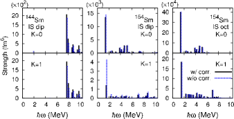
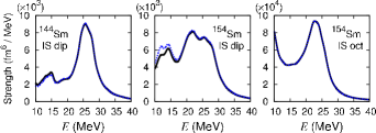
Figure 1: (Color online) The IS dipole and octupole transition-strength distributions in ¹⁴⁴Sm and in ¹⁵⁴Sm in the low-energy region (upper panels) and the GR energy region (lower). The results obtained with $\eta_{K}=0$ and $\eta_{K}^{(3)}=0$ are shown by dotted lines.

The isoscalar (IS) dipole operator, Eq. (9) contains the component of the center-of-mass motion. For deformed nuclei, the $K^{\pi}=0^{-}$ and $1^{-}$ octupole operators may also excite the spurious center-of-mass motion. To examine the mixing of the spurious modes, we use the corrected operator;

$$\hat{F}^{\tau=0}_{\lambda=1,K}=\sum_{\tau_{3}}\int d\bm{r}(r^{3}-\eta_{K}r)Y_{1K}(\hat{r})\hat{\psi}_{\tau_{3}}^{\dagger}(\bm{r})\hat{\psi}_{\tau_{3}}(\bm{r})$$ (15)

instead of using Eq. (9). Here, the correction factor in the isoscalar dipole operator originally discussed for a spherical system ($\eta$) to subtract the spurious component of the center-of-mass motion gia81 was extended to a deformed system ($\eta_{K}$) yos08 , and coincides with $\eta_{K}=\eta=5/3$ in the spherical limit. For the octupole operators, we use a similar technique to the case of the dipole operator yos09b ;

$$\hat{F}^{\tau=0}_{\lambda=3,K}=\sum_{\tau_{3}}\int d\bm{r}[r^{3}Y_{3K}(\hat{r})-\eta^{(3)}_{K}rY_{1K}(\hat{r})]\hat{\psi}_{\tau_{3}}^{\dagger}(\bm{r})\hat{\psi}_{\tau_{3}}(\bm{r}).$$ (16)

It is noted that the correction factor $\eta^{(3)}_{K}$ vanishes in the spherical limit.

In Fig. 1 we show the IS dipole and octupole transition-strength distributions in the low-energy region in ¹⁴⁴Sm and ¹⁵⁴Sm, calculated with and without the correction terms, $\eta_{K}$ and $\eta_{K}^{(3)}$. In ¹⁴⁴Sm, because the transition strengths calculated with finite $\eta_{K}$ are approximately identical to those with $\eta_{K}=0$, the low-energy dipole states around 8 MeV are almost free from the spurious center-of-mass motion. However, for the lowest $K=1$ dipole state in ¹⁵⁴Sm, we see a large difference between the two calculations. This implies that the full self-consistency is necessary to describe quantitatively the low-lying dipole states. The contamination of the spurious mode is smaller in the low-lying octupole excitations and in the GRs as shown in the lower panel of Fig. 1.

III.3 Giant resonances

Let us discuss properties of GRs. In order to quantify the excitation energy of the GR, two kinds of definition are utilized. The centroid energy $E_{c}$ is frequently used in the experimental analysis, defined by

$$E_{c}=\dfrac{m_{1}}{m_{0}},$$ (17)

where $m_{k}$ is a $k-$th moment of the transition strength distribution in an energy interval of $[E_{a},E_{b}]$ MeV.

$$m_{k}\equiv\int_{E_{a}}^{E_{b}}E^{k}S_{\lambda}^{\tau}(E)dE,$$ (18)

where $S^{\tau}_{\lambda}(E)$ is defined by Eq. (6) in the calculation. We take the upper and lower limits, $[E_{a},E_{b}]$, same as those used in the experimental analysis.

Another definition of the excitation energy is denoted as $E_{x}$. This is extracted by fitting the strength distribution of the GR, $S_{\lambda}^{\tau}(E)$, by the Lorentz curve with two parameters, the peak energy $E_{x}$ and the width $\Gamma$.

III.3.1 Positive-parity excitation

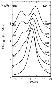
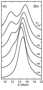
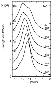
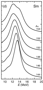
Figure 2: The strength distributions (shifted) of ISGMR [(a), (b)] and ISGQR [(c), (d)] in Nd and Sm isotopes.

Figure 2 shows the strength distributions of IS monopole and quadrupole excitations in the Nd and Sm isotopes. We discuss first the giant quadrupole resonance (GQR). Both in the Nd and Sm isotopes, ISGQRs are located around 12–14 MeV. With increase in the mass number, the peak energy of the ISGQR becomes smaller. This is consistent with the experiment on the systematic observation of the ISGQR energy in the Sm isotopes ito03 ; you04 . Figure 3 shows the centroid energy of the ISGQR in the Sm isotopes. Here we used the energy interval of [9,15] MeV. Open squares in Fig. 3 are obtained from the strength distribution in Ref. ito03 . The present results well reproduce the experimental data. The calculated centroid energy is well fitted by the $65.6A^{-1/3}$ line, which agrees with the empirical behavior, $(64.0\pm 1.7)\times A^{-1/3}$ har01 . Dependence on the choice of the Skyrme functional is discussed later.

The ISGQR in spherical nuclei was successfully described by the pairing-plus-quadrupole (P+Q) model. However, the same model failed to reproduce the observed data in deformed nuclei. This failure can be attributed to the violation of the nuclear self-consistency between the shapes of the potential and the density distributions. Making use of the quadrupole operator in doubly-stretched coordinates significantly improves the results kis75 . It is due to the fact that the doubly-stretched quadrupole operator appropriately describes the quadrupole fluctuation about a deformed ground state sak89a . In fact, the predicted deformation splitting of the ISGQR in ¹⁵⁴Sm is calculated to be about 2 MeV using the doubly-stretched P+Q model, whereas it is about 6 MeV using the ordinary P+Q model.

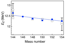
Figure 3: (Color online) The centroid energies of the ISGQR in the Sm isotopes with a fitted line. The experimental data itoh ; you04 are denoted by open symbols.

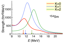
Figure 4: (Color online) The IS quadrupole transition-strength distribution in ¹⁵⁴Sm for the $K^{\pi}=0^{+}$, $1^{+}$, and $2^{+}$ excitations. The eigenenergies obtained with use of the doubly-stretched P+Q model are denoted by the arrows, and the peak position of the GQR was adjusted to the experimental data kis75 .

Figure 4 shows the IS quadrupole transition-strength distribution in ¹⁵⁴Sm for the $K^{\pi}=0^{+}$, $1^{+}$ and $2^{+}$ excitations. The $K$ splitting, $E_{K=2}-E_{K=0}$, for the ISGQR is 2.8 MeV in the present calculation. This is consistent with the value obtained in the doubly-stretched P+Q model and the experimental observation kis75 . This indicates that the present calculation based on the EDF naturally takes into account the nuclear self-consistency, which has to be introduced explicitly in the P+Q model where the higher-order terms are required additionally to satisfy the nuclear self-consistency sak89 . Since the energy splitting associated with the deformation is comparable to the smearing parameter, the deformation splitting, which is clearly visible in the photoabsorption cross sections yos11 , does not appear in the ISGQR. Instead, we find a broadening of the width for the ISGQR associated with the development of the deformation (see the table in Appendix B).

Next, let us discuss the monopole excitation. In the spherical nuclei, we can see a sharp peak at around 15 MeV which is identified as the ISGMR. In ¹⁴⁴Sm, the peak energy and the width are $E_{x}=14.8$ MeV and $\Gamma=2.61$ MeV. This is compatible with the observed values of $E_{x}=15.40\pm 0.30$ and $\Gamma=3.40\pm 0.20$ MeV you04 .

The ISGMR in deformed nuclei has a double-peak structure. The lower-energy peak ($8<E<13.5$ MeV) and the higher-energy peak ($13.5<E<19$ MeV) exhaust $31.4\%$ and $60.6\%$ of the IS monopole energy-weighted-sum rule (EWSR) value, $3.38\times 10^{5}$ fm⁴ MeV, in ¹⁵⁴Sm. The higher-energy peak of the IS monopole strength is identified as a primal ISGMR and the lower-energy peak is associated with the coupling to the $K^{\pi}=0^{+}$ component of the ISGQR. The lower peak of the ISGMR around 11 MeV, is located at the peak position of the $K^{\pi}=0^{+}$ component of the ISGQR shown in Fig. 4.

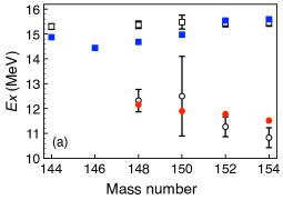
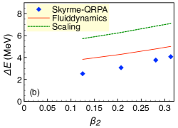
Figure 5: (Color online) (a)The excitation energies of the ISGMR in the Sm isotopes. The experimental data ito03 are denoted by open symbols with error bars. (b) The energy difference of the upper peak and the lower peak of the ISGMR in ^{148,150,152,154}Sm as a function of the deformation parameter $\beta_{2}$. The lines are results of the fluiddynamical and scaling models nis85 .

Table 2: The parameters of the ISGMR in ¹⁵⁴Sm. Fitting the strength function $S_{0}^{0}(E)$ with $\gamma=2$ MeV by a sum of two Lorentz lines, the peak energy $E_{x}$ and the width $\Gamma$ are extracted. The energy-weighted sum (EWS) of the transition strength is calculated in the energy range of [8,13.5] MeV and [13.5,19] MeV for the lower peak and upper peak of the ISGMR in the calculation using the SkM* functional. The energy range is slightly changed according to the shift of peak positions of the ISGMR in the calculations using the SLy4 and SkP functionals. The experimental values are taken from Refs. you04 and ito02 . Results of other calculations employing different kinds of model in Refs. nis85 and abg80 and are also included.

		Lower peak			Upper peak		Ratio of EWS
	$E_{x}$	$\Gamma$	EWS	$E_{x}$	$\Gamma$	EWS	Upper/Lower
	(MeV)	(MeV)	$\%$	(MeV)	(MeV)	$\%$
SkM*	11.5	3.75	31.4	15.6	2.73	60.6	1.9
SLy4	12.1	3.62	36.3	16.2	2.68	57.0	1.6
SkP	10.3	3.48	21.8	14.7	2.78	70.8	3.2
TAMU you04	$11.05\pm 0.05$	$3.2\pm 0.1$	$32\pm 2$	$15.17\pm 0.05$	$4.0\pm 0.1$	$80\pm 5$	$2.5\pm 0.2$
RCNP ito02	$11.0\pm 0.8$	(5.1)	$17.5\pm 5$	$15.6\pm 0.2$	(3.9)	$69\pm 5$	$3.9\pm 1.2$
Fluiddynamics nis85	10.1		21.5	15.6		76.3	3.5
Scaling nis85	11.0		16.6	18.1		83.4	5.0
Cranking abg80	10.4		21	15.9		79	3.8

Figure 5(a) shows the peak energy of the ISGMR in the Sm isotopes. The calculation shows an excellent agreement with the experimental data both in spherical and deformed nuclei. As the deformation develops from ¹⁴⁸Sm, the higher-energy peak of the ISGMR slightly increases. In Fig. 5(b), the energy difference of the upper and lower peaks of the ISGMR is shown as a function of the deformation parameter of the ground state. The results are compared with the predictions by the fluiddynamics model and the simple scaling model with the effective mass $m^{*}/m=0.8$ and the Landau parameter $F_{0}=-0.25$ nis85 . The result of the fluiddynamics model is consistent with our result, although it underestimates the excitation energy of the low-energy peak of ISGMR. The deformation dependence of the splitting energy is well reproduced. On the other hand, the simple scaling model significantly overestimates the ISGMR peak energy, which results in too large splitting of the peak energies.

Since the experimental studies for the detailed structure of the ISGMR in ¹⁵⁴Sm are available you04 ; ito02 , we are going to discuss here the properties of the calculated ISGMR in ¹⁵⁴Sm. Table 2 summarizes the parameters of the ISGMR in ¹⁵⁴Sm. The peak energy $E_{x}$ and the width $\Gamma$ in a deformed system are obtained by fitting the strength distribution with a sum of two Lorentz lines. The calculations are compared with inelastic $\alpha$ scattering experiments at Texas A$\&$M University you04 and at RCNP, Osaka University ito02 . Results of the calculations employing the SLy4 cha98 and SkP dob84 functionals and other models abg80 ; nis85 are also shown. The same pairing energy functional, Eq. (3), is used in all the calculations.

The excitation energies are described best by the SkM* functional among three kinds of functionals. The ratio of the energy-weighted sum of the strengths for the upper peak to that for the lower peak varies from 1.6 (SLy4) to 3.2 (SkP), and the SkP gives better agreement with the experimental data. This implies that the coupling effect between the GMR and the GQR is weaker for the SkP functional than for the SkM* and SLy4 functionals. As discussed above, the coupling is determined by the quadrupole moment (deformation parameter) of the ground state. Indeed, the mass deformation parameter obtained in the present calculation is $\beta_{2}=0.29$ for SkP, while $\beta_{2}=0.31$ for SkM* and SLy4.

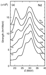
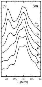
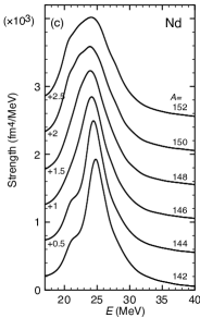
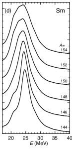
Figure 6: The strength distributions (shifted) of IVGMR [(a), (b)] and IVGQR [(c), (d)] in Nd and Sm isotopes.

Figure 6 shows the strength distributions for the isovector (IV) monopole and quadrupole excitations. Although the experimental data for the IVGMR and IVGQR are unavailable in the mass region under investigation, the present calculation suggests the existence of these GR modes in the Nd and Sm isotopes. The energy of IVGQR is approximately fitted by $129.5$ and $130.3$ $\times A^{-1/3}$ MeV for Nd and Sm isotopes, respectively. This is consistent with the experimental observations $\sim 130A^{-1/3}$ MeV in $A=140-240$ nuclei hen11 . The $K$-splitting of the IVGQR in deformed nuclei is invisible because the $K$-splitting is small.

A double-peak structure can be seen in deformed nuclei for the IVGMR as well as for the ISGMR. The lower peak around 20 MeV in the deformed nuclei emerges associated with the coupling to the $K^{\pi}=0^{+}$ component of the IVGQR. The upper peak around 30 MeV may be identified as a primal IVGMR because the resonance peak appears in this energy region in the spherical nuclei. Similarly to the ISGMR, the upper peak of the IVGMR is upward-shifted with increasing the neutron number. This is due to the stronger coupling between the IVGMR and the IVGQR in nuclei with larger deformation. The energy difference between the upper and lower peaks of the IVGQR in ¹⁵⁴Sm approaches about 10 MeV, which is more than twice as large as the energy difference seen in the ISGMR.

III.3.2 Negative-parity excitation

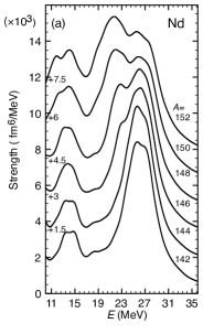
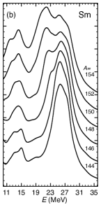
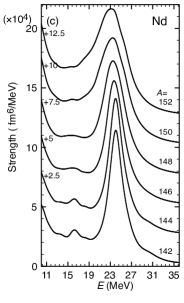
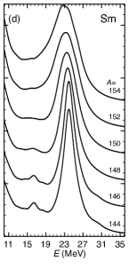
Figure 7: Strength distributions (shifted) of ISGDR [(a), (b)] and ISGOR (HEOR) [(c), (d)] in Nd and Sm isotopes.

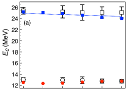
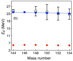
Figure 8: (Color online) (a) The centroid energies of the low-energy and high-energy components of the ISGDR in the Sm isotopes. (b) The centroid energies of the HEOR and the LEOR in the Sm isotopes. The centroid energy of LEOR is evaluated in the energy range of $[E_{a},E_{b}]=[3,10]$ MeV. The dotted line is obtained by fitting the results with an $A^{-1/3}$ line. The experimental data ito03 are denoted by open symbols with error bars.

Figure 7 shows the strength distributions of the IS compression dipole and octupole excitations. In the IS octupole-transition-strength distributions, we can see a high-energy octupole resonance (HEOR) at around 25 MeV. Furthermore, we find a broadening of the width associated with the deformation as observed in the experiment mor82 . We show the centroid energy of the HEOR and the low-energy octupole resonance (LEOR) in the Sm isotopes in Fig. 8(b). The centroid energy of HEOR and LEOR is evaluated in the energy range of [17, 33] MeV and [3,10] MeV, respectively. The calculated energy of HEOR is best fitted to a $124.8\times A^{-1/3}$ line, and agrees with the experimental observation ito03 . However, this excitation energy is significantly higher than the systematic value of $110\pm 5\times A^{-1/3}$ MeV har01 .

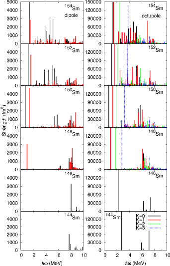
Figure 9: (Color online) The low-energy IS dipole and octupole transition strengths in the Sm isotopes. The strengths with different $K$ are all identical for the spherical nuclei.

Below 10 MeV, we find low-lying collective (discrete) states and the LEOR. The right panels of Fig. 9 show the low-energy part of the IS octupole transition-strengths in the Sm isotopes. We find that the low-lying collective $K=2,3$ states are overlapping with the LEOR in the well-deformed nuclei. The present calculation gives 6.5$\%$ and 24$\%$ of the IS octupole EWSR value in ¹⁵⁴Sm for the energy intervals $0-3$ MeV and $0-7$ MeV, respectively. This is compatible to the experimental value of 7$\%$ and 19$\%$ for the discrete states only and for the low-lying states including the discrete levels and the LEOR, respectively mos76 . The early theoretical calculation employing the pairing plus octupole interaction model gives also an excellent agreement with the observed value by adjusting the interaction strengths mal77 .

The calculated octupole strength carries $51-53$ % of the EWSR value in the HEOR energy region of $17-33$ MeV. On the contrary, the experiment ito03 has reported decrease of the strength in the same energy region from 75% to 30% of EWSR as increasing the mass number in the Sm isotopes. This inconsistency may be attributed to the uncertainty of the choice of the continuum in the experimental analysis and the strong overlap with the ISGDR har01 .

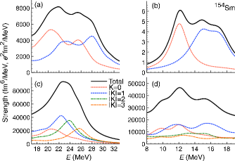
Figure 10: (Color online) (a) The IS compression dipole strength distribution in the ISGDR energy region in ¹⁵⁴Sm. (b) The IV dipole strength distribution in the GDR energy region. (c) The IS octupole strength distribution. (d) The IV octupole strength distribution.

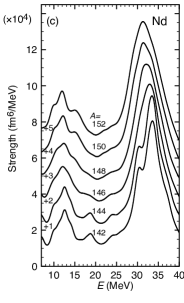
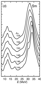
Figure 11: The strength distributions (shifted) of IVGDR [(a), (b)] and IVGOR [(c), (d)]in Nd and Sm isotopes.

We have the ISGDR at around 25 MeV corresponding to the $3\hbar\omega$ excitation, and this energy region is where the HEOR is located. We show the centroid energy of the ISGDR in the Sm isotopes in Fig. 8(a). The calculated energy is best fitted to the $130.7\times A^{-1/3}$ line. The fitted energy of the ISGDR is slightly higher than that of the HEOR. The ISGDR in spherical nuclei is investigated in the framework of the HF-BCS + QRPA approach employing several Skyrme functionals col00 . The excitation energy obtained in Ref. col00 in ¹⁴⁴Sm is consistent with our result.

A deformation effect on the ISGDR can be seen in the increase of its width. This is due to the deformation splitting of the $K=0$ and 1 components of the ISGDR similarly in the photoabsorption cross sections. Furthermore, the width becomes even larger due to the coupling to the $K=0$ and 1 components of the HEOR. Figures 10(a) and (c) show the strength distributions of the IS dipole and octupole excitations in ¹⁵⁴Sm. The resonance structure at $26-28$ MeV appears due to the deformation splitting of the primal ISGDR, and the structure at $20-23$ MeV is due to the coupling to the $K=0,1$ components of the HEOR. Because of these two effects, the total strength distribution becomes very broad. When we fit the calculated strength distribution with a Lorentz line in the energy region of [15, 35] MeV, we obtain the width $\Gamma=13.4$ MeV. The large width is observed experimentally as $22.6\pm 4.2$ MeV in Ref. ito03 , while the rather small width ($11.8\pm 0.5$ MeV) is reported in Ref. you04 .

We furthermore find a low-energy (LE) ISGDR at about 14 MeV. We also find that the low-lying dipole states appear below 5 MeV with possession of large transition strengths in the deformed systems as shown in the left panels of Fig. 9. This is due to the coupling to the low-lying octupole modes of excitation.

The strength distribution in ¹⁵⁴Sm obtained by the $(\alpha,\alpha^{\prime})$ experiment in Ref. you04 shows a three-peak structure at around the excitation energy of $12-16$ MeV, $20-24$ MeV and $26-29$ MeV. The data were compared with the fluiddynamics results of Ref. nis85 , however, the mechanism for appearance of the second peak was unclear. According to the present calculation, it is suggested that the first peak corresponds to the low-energy ISGDR, the second peak is associated with the coupling to the $K=0$ and $1$ components of the HEOR, and the third peak is the primal ISGDR.

Figure 11 shows the strength distributions of IV dipole and octupole excitations. The IV giant octupole resonance (GOR) is seen above 30 MeV, and we find a bump structure at around 10 MeV corresponding to the IV-LEOR. The strength is rather smaller than that of the IV-HEOR. Noted that the strength of the IS-LEOR is compatible to that of the IS-HEOR.

In the deformed systems, we see an appearance of the shoulder structure at about 15 MeV. Figure 10 (b) and (d) presenting the IV dipole and octupole strength distributions in ¹⁵⁴Sm show that the shoulder structure is associated with the deformation splitting of the GDR and its coupling to the IV-LEOR.

III.3.3 Low-lying collective states

Figure 12: The excitation energies of the lowest $K^{\pi}=0^{+}$, $2^{+}$, $0^{-}$ and $1^{-}$ states in Nd and Sm isotopes. The experimental data for Nd and Sm isotopes ENSDF are denoted by open triangles and circles, respectively. The lines are drawn to guide the eyes.

In this subsection, we are going to discuss the low-lying states. As shown in Fig. 9, we see an appearance of the collective mode for the IS dipole excitation below 2 MeV associated with an onset of deformation. This is due to the strong coupling to the collective octupole mode of excitation.

What has to be mentioned here is an absence of the collective $K=0$ mode in ¹⁴⁸Sm. In the present calculation, we have two imaginary solutions in the $K^{\pi}=0^{-}$ channel, one of which is associated with the spurious center-of-mass motion. In ¹⁵⁰Sm, we have the $K=0$ mode at 0.72 MeV. The excitation energy of the collective $K=0$ mode becomes higher when increasing the neutron number. Thus, we can consider that the second imaginary solution in ¹⁴⁸Sm indicates the instability against the axially-symmetric octupole deformation. In fact, the largest $B(E3;0_{1}^{+}\to 3_{1}^{-})$ value is measured in ¹⁴⁸Sm among the even-even Sm isotopes ENSDF .

Before going to the next subsection, we summarize the energy of the low-lying collective states in the spherical and the well-deformed Nd and Sm isotopes. Figure 12 shows the excitation energies of the lowest $K^{\pi}=0^{+}$, $2^{+}$, $0^{-}$ and $1^{-}$ states. The available experimental data ENSDF are also shown. For the experimental values, we neglect the rotational correction, which is $30$ keV at most in ¹⁵⁴Sm. Figure 12 shows that the observed isotopic dependence is well reproduced.

The excitation energies of the quadrupole-vibrational states agree with the experimental data within $0.5-1$ MeV. This result is close to the one obtained in Ref. ter11 , where they obtained the $\gamma$-vibrational state at 2.5 MeV and at 2.3 MeV in ¹⁵²Nd and in ¹⁵⁴Sm, respectively despite the use of a different pairing functional from ours. Reproduction of the experimental values of the octupole-vibrational states in the deformed nuclei is extremely good.

Table 3: The excitation energies (in units of MeV) of the low-lying collective states in ¹⁵⁴Sm. Experimental data are taken from Ref. ENSDF .

	$K^{\pi}=0^{+}$	$K^{\pi}=2^{+}$	$K^{\pi}=0^{-}$	$K^{\pi}=1^{-}$
SkM*	1.55	1.93	1.37	1.49
SLy4	1.46	1.81	1.25	1.66
SkP	0.95	0.92	1.44	1.64
Exp.	1.099	1.440	0.921	1.475

Table 3 summarizes the excitation energy of the low-lying collective states in ¹⁵⁴Sm obtained by the QRPA calculations employing the different kinds of Skyrme functionals. All the Skyrme functionals under consideration give a reasonable agreement with the measurements, and the quality is at the same level found in Ref. ter10 .

III.4 Incompressibility and effective mass in GRs

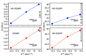
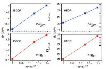
Figure 13: (Color online) The peak energies of the ISGMR and ISGQR, and the centroid energy of the ISGDR and HEOR in ¹⁴⁴Sm and ¹⁵⁴Sm obtained by employing the Skyrme functionals giving the different nuclear-matter properties. The continuous lines are drawn to guide the eyes. Experimental data are shown by the open square ito03 and the circle you04 with the error bars.

In this subsection, we investigate how the calculated properties of the GRs depend on the Skyrme EDFs with the different nuclear matter properties, effective mass and the incompressibility. We take ¹⁴⁴Sm and ¹⁵⁴Sm as examples of spherical and deformed nuclei, respectively. The experimental data for all the isoscalar multipole excitations are available for these isotopes. Nuclear matter and deformation properties for the functionals we employ are listed in Table 4.

Table 4: The nuclear matter and deformation properties for the Skyrme functionals under consideration. The table represents the isoscalar effective mass $m^{*}_{0}/m$, the nuclear-matter incompressibility $K$, and the deformation parameters $\beta_{2}$ in ¹⁵⁴Sm.

Forces	$m^{*}_{0}/m$	$K$ (MeV)	$\beta_{2}^{\nu}$	$\beta_{2}^{\pi}$
SkM*	0.79	216.7	0.30	0.33
SLy4	0.70	229.9	0.30	0.33
SkP	1.00	201.0	0.28	0.30

As we discussed in Section III.3.1, the experimental value for the peak energies of the ISGMR is fairly reproduced in the calculation for all the functionals under investigation. The excitation energies of the upper peak of the ISGMR in ¹⁵⁴Sm and the ISGMR in ¹⁴⁴Sm are shown in the upper-left panels of Fig. 13 as functions of the square root of the incompressibility. We can see a clear correlation between them. This result is consistent with the fact that the GMR energy is proportional to the square root of the incompressibility bla80 . The excitation energy is given in the scaling model as

$$\omega^{s}_{\mathrm{M}}=\sqrt{5(m/m^{*}_{0})(1+F_{0})}\Omega=\sqrt{5K/3m\langle r^{2}\rangle},$$ (19)

where $F_{0}$ is the Landau-Migdal parameter and $\hbar\Omega\simeq 41A^{-1/3}$ (MeV) nis85 , and the excitation energy of the upper peak of the ISGMR in deformed systems is given in Eq. (3.10) of Ref. nis85 . Note here that as we saw in Sec. III.3.1 the scaling model overestimates the energy of the compressible modes, while it gives the qualitative understanding of GRs nis85 . Since the SkP functional has a small incompressibility, the calculated excitation energy of the ISGMR is lower than the experimental data and the results obtained by using the SkM* and SLy4 functionals.

For the GMR in ¹⁵⁴Sm, the SkM* functional gives the excitation energy which is very close to the observation ito03 . However, in ¹⁴⁴Sm the SkM* underestimates the observation, and the SLy4 gives the reasonable energy. The experimental data reported in Refs. you99 ; you04 for the GMR centroid energy in ¹⁴⁴Sm are $15.39\pm 0.28$ MeV and $15.40\pm 0.30$ MeV. Therefore, the present calculation suggests that the nuclear-matter incompressibility is about $15.2^{2}=231$ MeV deduced from the comparison for ¹⁴⁴Sm and $14.6^{2}=213$ MeV for ¹⁵⁴Sm. As mentioned in Section III.1, the pairing properties in ¹⁴⁴Sm and ¹⁵⁴Sm are quite different. Thus it would be interesting to investigate in detail the pairing effects on the GMR li08 ; kha10 , taking the deformation effect into account.

The upper-right panel of Fig. 13 shows the the centroid energy of the ISGDR. Here, we evaluate the centroid energy in the energy region of the second and the third peaks as done in the experimental analysis ito03 ; you04 for ¹⁵⁴Sm. The excitation energy of the ISGDR is given in the scaling model as nis85

$$\omega_{\mathrm{D}}^{s}=\sqrt{\dfrac{7}{3}\left[\dfrac{5K}{3m\langle r^{2}\rangle}+\dfrac{8}{5}\left(\dfrac{m}{m^{*}_{0}}\right)\right]}\Omega.$$ (20)

It contains information not only of the incompressibility but of the effective mass. Note that the primal ISGDR in the deformed nuclei is the third peak as we discussed in the previous section.

In the left-lower and right-lower panels of Fig. 13, we show the peak energy of the ISGQR and the centroid energy of the HEOR as functions of the inverse of square root of the isoscalar effective mass $\sqrt{m^{*}_{0}/m}^{-1}$. We can see a linear correlation between them: The smaller the isoscalar effective mass, the higher the resonance energy. This is consistent with the results of the simple model. The excitation energy of the ISGQR and HEOR is given by the scaling model as nis85

$$\omega^{s}_{\mathrm{Q}} =\sqrt{2(m/m^{*}_{0})}\Omega,$$ (21)

$$\omega^{s}_{\mathrm{O}} =\sqrt{(28/5)(m/m^{*}_{0})}\Omega.$$ (22)

This feature is also consistent with the finding in the GQR energy obtained by the RPA calculations for spherical systems rei99 .

For the ISGQR, the effective mass $m^{*}_{0}/m$ around $1.09^{-2}=0.84$ gives the excitation energy which is compatible with the experimental results both in ¹⁴⁴Sm and in ¹⁵⁴Sm. For the HEOR in ¹⁴⁴Sm, slightly smaller effective mass around $1.16^{-2}=0.74$ seems to be favored in comparison with the experimental observation ito03 . In ¹⁵⁴Sm, it is hard to deduce the optimal value for the effective mass due to the large error in the experiment ito03 .

The excitation energies of the HEOR in ¹⁴⁴Sm and ¹⁵⁴Sm reported in Ref. you04 are $19.6\pm 0.5$ MeV and $18.5\pm 0.5$ MeV, respectively. The error is much smaller than that in the experiment at RCNP ito03 . However, the excitation energy is small and it is outside of the energy region obtained by the three types of Skyrme functionals. This indicates that the effective mass is around $0.95^{-2}=1.11$ or even larger. Since the strength distribution of the ISGDR in Ref. you04 looks similar to our results, the large discrepancy found in the HEOR is difficult to understand.

IV Summary

We have investigated the deformation effects on GRs in the rare-earth nuclei by employing the newly developed parallelized computer code for the QRPA based on the Skyrme EDF. We found a good scalability for the calculation of the matrix elements of the QRPA equation by the use of a two-dimensional block cyclic distribution, which is suited for the ScaLAPACK.

The axial deformation in the ground state allows the GRs with the multipolarity $L=0$ and $2$ to mix in the $K^{\pi}=0^{+}$ channel. Accordingly, we have obtained a double-peak structure of the ISGMR. The energy difference between the upper and lower peaks in the ISGMR and the fraction of the energy-weighted summed strength in the lower peak can be a sensitive measure of the ground-state quadrupole moment. We also predict a prominent double-peak structure of the IVGMR.

For the negative-parity excitations, the excitation modes with $L=1$ and $3$ can mix in the $K^{\pi}=0^{-}$ and $1^{-}$ channels. This mixing leads to a large width for the ISGDR and the enhancement of the low-lying dipole-transition strengths associated with coupling to the collective octupole mode of excitation. In the IV channel, the excitation energies of GDR and LEOR are similar. In deformed nuclei, the coupling between these two modes creates a broadening of the IV-LEOR peak.

It should be emphasized here that the origin of the observed peak splitting in the IVGDR is different from that of the other GRs. The double-peak structure in the IVGDR is well-known to be due to a direct consequence of the nuclear deformation BM2 . Namely, this is associated with different frequencies between $K=0$ and $K=1$ modes in the axially deformed system. The same kind of deformation splitting, according to the different $K$ quantum numbers, also exists in the other GRs, however, its magnitude is much smaller than the IVGDR. Typically, the magnitude of the $K$-splitting is about 2 MeV. Therefore, with the smearing width of $\gamma=2$ MeV in the present calculation, the peak splitting disappears. The double-peak structures in deformed nuclei for ISGMR, IVGMR, ISGDR, and IV-LEOR, observed in the present calculation are all associated with the coupling among GRs with different multipolarity.

Calculations using several commonly used Skyrme functionals in the nuclear EDF method all give a fairly good reproduction of the experimental data, not only for the GRs but also for the low-lying collective modes in the spherical and the well deformed nuclei. Comparison of the GR results with the experimental data obtained at RCNP ito03 and TAMU you04 was performed in details for the spherical nucleus ¹⁴⁴Sm and the deformed ¹⁵⁴Sm. The experimental data for the ISGMR and the ISGDR indicates the incompressibility around $210-230$ MeV. The excitation energy of the ISGQR is well reproduced with the effective mass $m^{*}_{0}/m\simeq 0.8-0.9$ both in ¹⁴⁴Sm and in ¹⁵⁴Sm. The experimental data for the HEOR are very different between the two experiments ito03 ; you04 . A further experiments for HEOR are needed to confirm the value of the effective mass.

Appendix A QRPA matrix elements

Using the quasiparticle wave functions $\varphi_{1}(\bm{r}\sigma)$ and $\varphi_{2}(\bm{r}\sigma)$, the solutions of the coordinate-space HFB equation, the matrix elements appearing in the QRPA matrix are written as

$$A_{\alpha\beta\gamma\delta}=(E_{\alpha}+E_{\beta})\delta_{\alpha\gamma}\delta_{\beta\delta}$$

$$+\sum_{\sigma_{1},\sigma_{2},\sigma_{1}^{\prime},\sigma_{2}^{\prime}}\int d\bm{r}_{1}d\bm{r}_{2}d\bm{r}_{1}^{\prime}d\bm{r}_{2}^{\prime}\times$$

$$\{\varphi_{1,\alpha}(\bm{r}_{1}\bar{\sigma_{1}})\varphi_{1,\beta}(\bm{r}_{2}\bar{\sigma_{2}})\bar{v}_{pp}(12;1^{\prime}2^{\prime})\varphi^{*}_{1,\gamma}(\bm{r}_{1}^{\prime}\bar{\sigma_{1}^{\prime}})\varphi^{*}_{1,\delta}(\bm{r}_{2}^{\prime}\bar{\sigma_{2}^{\prime}})$$

$$+\varphi_{2,\alpha}(\bm{r}_{1}\sigma_{1})\varphi_{2,\beta}(\bm{r}_{2}\sigma_{2})\bar{v}_{pp}(12;1^{\prime}2^{\prime})\varphi^{*}_{2,\gamma}(\bm{r}_{1}^{\prime}\sigma_{1}^{\prime})\varphi^{*}_{2,\delta}(\bm{r}_{2}^{\prime}\sigma_{2}^{\prime})$$

$$-\varphi_{1,\alpha}(\bm{r}_{1}\bar{\sigma_{1}})\varphi^{*}_{2,\gamma}(\bm{r}_{2}\sigma_{2})\bar{v}_{ph}(12;1^{\prime}2^{\prime})\varphi_{2,\beta}(\bm{r}_{1}^{\prime}\sigma_{1}^{\prime})\varphi^{*}_{1,\delta}(\bm{r}_{2}^{\prime}\bar{\sigma_{2}^{\prime}})$$

$$-\varphi_{1,\beta}(\bm{r}_{1}\bar{\sigma_{1}})\varphi^{*}_{2,\delta}(\bm{r}_{2}\sigma_{2})\bar{v}_{ph}(12;1^{\prime}2^{\prime})\varphi_{2,\alpha}(\bm{r}_{1}^{\prime}\sigma_{1}^{\prime})\varphi^{*}_{1,\gamma}(\bm{r}_{2}^{\prime}\bar{\sigma_{2}^{\prime}})$$

$$+\varphi_{1,\alpha}(\bm{r}_{1}\bar{\sigma_{1}})\varphi^{*}_{2,\delta}(\bm{r}_{2}\sigma_{2})\bar{v}_{ph}(12;1^{\prime}2^{\prime})\varphi_{2,\beta}(\bm{r}_{1}^{\prime}\sigma_{1}^{\prime})\varphi^{*}_{1,\gamma}(\bm{r}_{2}^{\prime}\bar{\sigma_{2}^{\prime}})$$

$$+\varphi_{1,\beta}(\bm{r}_{1}\bar{\sigma_{1}})\varphi^{*}_{2,\gamma}(\bm{r}_{2}\sigma_{2})\bar{v}_{ph}(12;1^{\prime}2^{\prime})\varphi_{2,\alpha}(\bm{r}_{1}^{\prime}\sigma_{1}^{\prime})\varphi^{*}_{1,\delta}(\bm{r}_{2}^{\prime}\bar{\sigma_{2}^{\prime}})\},$$ (23)

$$B_{\alpha\beta\gamma\delta}=\sum_{\sigma_{1},\sigma_{2},\sigma_{1}^{\prime},\sigma_{2}^{\prime}}\int d\bm{r}_{1}d\bm{r}_{2}d\bm{r}_{1}^{\prime}d\bm{r}_{2}^{\prime}\times$$

$$\{-\varphi_{1,\alpha}(\bm{r}_{1}{\bar{\sigma}_{1}})\varphi_{1,\beta}(\bm{r}_{2}{\bar{\sigma}_{2}})\bar{v}_{pp}(12;1^{\prime}2^{\prime})\varphi_{2,\bar{\gamma}}(\bm{r}_{1}^{\prime}\sigma_{1}^{\prime})\varphi_{2,\bar{\delta}}(\bm{r}_{2}^{\prime}\sigma_{2}^{\prime})$$

$$-\varphi_{2,\alpha}(\bm{r}_{1}\sigma_{1})\varphi_{2,\beta}(\bm{r}_{2}\sigma_{2})\bar{v}_{pp}(12;1^{\prime}2^{\prime})\varphi_{1,\bar{\gamma}}(\bm{r}_{1}^{\prime}{\bar{\sigma}_{1}^{\prime}})\varphi_{1,\bar{\delta}}(\bm{r}_{2}^{\prime}{\bar{\sigma}_{2}^{\prime}})$$

$$+\varphi_{1,\alpha}(\bm{r}_{1}{\bar{\sigma}_{1}})\varphi_{1,\bar{\gamma}}(\bm{r}_{2}{\bar{\sigma}_{2}})\bar{v}_{ph}(12;1^{\prime}2^{\prime})\varphi_{2,\beta}(\bm{r}_{1}^{\prime}\sigma_{1}^{\prime})\varphi_{2,\bar{\delta}}(\bm{r}_{2}^{\prime}\sigma_{2}^{\prime})$$

$$+\varphi_{1,\beta}(\bm{r}_{1}{\bar{\sigma}_{1}})\varphi_{1,\bar{\delta}}(\bm{r}_{2}{\bar{\sigma}_{2}})\bar{v}_{ph}(12;1^{\prime}2^{\prime})\varphi_{2,\alpha}(\bm{r}_{1}^{\prime}\sigma_{1}^{\prime})\varphi_{2,\bar{\gamma}}(\bm{r}_{2}^{\prime}\sigma_{2}^{\prime})$$

$$-\varphi_{1,\alpha}(\bm{r}_{1}{\bar{\sigma}_{1}})\varphi_{1,\bar{\delta}}(\bm{r}_{2}{\bar{\sigma}_{2}})\bar{v}_{ph}(12;1^{\prime}2^{\prime})\varphi_{2,\beta}(\bm{r}_{1}^{\prime}\sigma_{1}^{\prime})\varphi_{2,\bar{\gamma}}(\bm{r}_{2}^{\prime}\sigma_{2}^{\prime})$$

$$-\varphi_{1,\beta}(\bm{r}_{1}{\bar{\sigma}_{1}})\varphi_{1,\bar{\gamma}}(\bm{r}_{2}{\bar{\sigma}_{2}})\bar{v}_{ph}(12;1^{\prime}2^{\prime})\varphi_{2,\alpha}(\bm{r}_{1}^{\prime}\sigma_{1}^{\prime})\varphi_{2,\bar{\delta}}(\bm{r}_{2}^{\prime}\sigma_{2}^{\prime})\}.$$ (24)

Here, the time-reversed state is defined as

$$\varphi_{\bar{i}}(\bm{r}\sigma)=-2\sigma\varphi_{i}^{*}(\bm{r}-\sigma).$$ (25)

If one assumes that the effective pairing interaction is local, $\bar{v}_{pp}$ is written as

$$\bar{v}_{pp}(12;1^{\prime}2^{\prime})= V_{pp}(\bm{r}_{1}\sigma_{1}\tau_{1},\bm{r}_{2}\sigma_{2}\tau_{2})\times$$

$$\delta(\bm{r}_{1}^{\prime}-\bm{r}_{1})\delta_{\sigma_{1}^{\prime},\sigma_{1}}\delta_{\tau_{1}^{\prime},\tau_{1}}\delta(\bm{r}_{2}^{\prime}-\bm{r}_{2})\delta_{\sigma_{2}^{\prime},\sigma_{2}}\delta_{\tau_{2}^{\prime},\tau_{2}},$$ (26)

and for $V_{pp}$ we use the form

$$V_{pp}(\bm{r}_{1}\sigma_{1}\tau_{1},\bm{r}_{2}\sigma_{2}\tau_{2})= V_{0}\mathrm{g}_{q}[\varrho(\bm{r}_{1}),\varrho_{1}(\bm{r}_{1})]\times$$

$$\delta(\bm{r}_{1}-\bm{r}_{2})\delta_{\sigma_{1},-\sigma_{2}}\delta_{\tau_{1},\tau_{2}}.$$ (27)

in the present paper.

Similarly, the effective interaction for the p-h channel reads

$$\bar{v}_{ph}(12;1^{\prime}2^{\prime})= V_{ph}(\bm{r}_{1}\sigma_{1}\tau_{1},\bm{r}_{2}\sigma_{2}\tau_{2})\times$$

$$\delta(\bm{r}_{1}^{\prime}-\bm{r}_{1})\delta_{\sigma_{1}^{\prime},\sigma_{1}}\delta_{\tau_{1}^{\prime},\tau_{1}}\delta(\bm{r}_{2}^{\prime}-\bm{r}_{2})\delta_{\sigma_{2}^{\prime},\sigma_{2}}\delta_{\tau_{2}^{\prime},\tau_{2}},$$ (28)

and we take the form

$$V_{ph}(\bm{r}_{1}\sigma_{1}\tau_{1},\bm{r}_{2}\sigma_{2}\tau_{2})=$$

$$(a_{0}+a_{0}^{\prime}\bm{\tau}_{1}\cdot\bm{\tau}_{2}+(b_{0}+b_{0}^{\prime}\bm{\tau}_{1}\cdot\bm{\tau}_{2})\bm{\sigma}_{1}\cdot\bm{\sigma}_{2})\delta(\bm{r}_{1}-\bm{r}_{2})$$

$$+(a_{1}+a_{1}^{\prime}\bm{\tau}_{1}\cdot\bm{\tau}_{2}+(b_{1}+b_{1}^{\prime}\bm{\tau}_{1}\cdot\bm{\tau}_{2})\bm{\sigma}_{1}\cdot\bm{\sigma}_{2})$$

$$\times(\bm{k}^{\dagger 2}\delta(\bm{r}_{1}-\bm{r}_{2})+\delta(\bm{r}_{1}-\bm{r}_{2})\bm{k}^{2})$$

$$+(a_{2}+a_{2}^{\prime}\bm{\tau}_{1}\cdot\bm{\tau}_{2}+(b_{2}+b_{2}^{\prime}\bm{\tau}_{1}\cdot\bm{\tau}_{2})\bm{\sigma}_{1}\cdot\bm{\sigma}_{2})$$

$$\times(\bm{k}^{\dagger}\cdot\delta(\bm{r}_{1}-\bm{r}_{2})\bm{k})$$

$$+(a_{4}+a_{4}^{\prime}\bm{\tau}_{1}\cdot\bm{\tau}_{2})(\bm{\sigma}_{1}+\bm{\sigma}_{2})\cdot\bm{k}^{\dagger}\times\delta(\bm{r}_{1}-\bm{r}_{2})\bm{k}$$ (29)

with the standard notations of $\bm{k}$ and $\bm{k}^{\dagger}$. The coefficients in Eq. (29) are given in Ref. ter05 . The coefficients $a_{0},a_{0}^{\prime},b_{0}$ and $b_{0}^{\prime}$ are density dependent and include the rearrangement terms. In the present paper, we have an additional contribution to these terms coming from the pairing EDF (3). They are

$$\left\{\begin{array}[]{lll}-\dfrac{V_{0}}{2}\dfrac{\eta_{2}}{\varrho_{0}^{2}}[\tilde{\varrho}_{\nu}^{2}(\bm{r})+\tilde{\varrho}_{\pi}^{2}(\bm{r})]&(\mathrm{for}&\nu-\nu,\pi-\pi)\\ \dfrac{V_{0}}{2}\dfrac{\eta_{2}}{\varrho_{0}^{2}}[\tilde{\varrho}_{\nu}^{2}(\bm{r})+\tilde{\varrho}_{\pi}^{2}(\bm{r})]&(\mathrm{for}&\nu-\pi).\end{array}\right.$$ (32)

Appendix B Parameters of the giant resonances

We summarize here the peak energy and the width of the GRs obtained by the calculations with the SkM* functional.

Table 5: The parameters of the ISGMR and IVGMR.

	ISGMR				IVGMR
	$E_{x}$	$\Gamma$	$E_{x}$	$\Gamma$	$E_{x}$	$\Gamma$	$E_{x}$	$\Gamma$
	(MeV)	(MeV)	(MeV)	(MeV)	(MeV)	(MeV)	(MeV)	(MeV)
142Nd			15.0	2.67			30.0	10.7
144Nd			14.5	2.79			29.6	10.2
146Nd	12.1	2.37	14.8	3.05	21.9	7.47	29.7	9.68
148Nd	11.9	2.83	15.0	3.05	21.7	4.54	29.8	9.39
150Nd	11.8	3.22	15.6	3.15	21.1	3.92	30.2	9.81
152Nd	11.5	3.40	15.7	3.20	20.7	3.91	30.3	9.76
144Sm			14.9	2.62			29.9	10.9
146Sm			14.4	2.68			29.4	10.4
148Sm	12.2	2.07	14.7	2.97	21.4	6.28	29.5	10.0
150Sm	11.9	2.79	15.0	2.97	21.6	4.27	29.8	9.52
152Sm	11.8	3.20	15.5	3.04	21.2	3.79	30.2	9.90
154Sm	11.5	3.39	15.6	3.12	20.9	3.77	30.3	9.80

Table 6: The parameters of the ISGDR and IVGDR.

	LE-ISGDR		ISGDR				IVGDR
	$E_{x}$	$\Gamma$	$E_{x}$	$\Gamma$	$E_{x}$	$\Gamma$	$E_{x}$	$\Gamma$	$E_{x}$	$\Gamma$
	(MeV)	(MeV)	(MeV)	(MeV)	(MeV)	(MeV)	(MeV)	(MeV)	(MeV)	(MeV)
142Nd	14.2	7.62	26.0	6.32			14.8	4.40
144Nd	13.9	8.25	25.9	6.33			14.8	4.34
146Nd	13.8	8.90	23.4	7.49	26.7	5.15	14.1	3.65	17.0	3.20
148Nd	13.8	9.26	22.3	5.78	26.7	5.71	13.5	3.58	16.5	4.73
150Nd	13.7	11.3	21.7	7.62	27.1	5.74	12.4	2.56	15.7	5.65
152Nd	13.6	14.1	21.1	9.26	27.2	6.63	12.0	2.56	15.7	5.69
144Sm	14.3	9.52	25.9	6.20			14.8	4.38
146Sm	13.9	10.5	25.8	6.21			14.8	4.31
148Sm	14.0	10.3	23.6	7.59	26.7	4.95	14.1	3.58	16.9	3.45
150Sm	14.0	9.77	22.2	5.69	26.6	5.87	13.3	3.30	16.0	4.96
152Sm	14.0	10.8	21.4	6.44	26.8	7.87	12.4	2.46	15.7	5.68
154Sm	14.0	12.6	21.0	8.21	26.9	7.44	12.1	2.51	15.7	5.70

Table 7: The parameters of the ISGQR and IVGQR.

	ISGQR		IVGQR
	$E_{x}$	$\Gamma$	$E_{x}$	$\Gamma$
	(MeV)	(MeV)	(MeV)	(MeV)
142Nd	13.3	2.89	24.8	5.20
144Nd	12.9	2.93	24.5	5.12
146Nd	12.7	3.01	24.0	5.71
148Nd	12.6	3.51	23.5	6.69
150Nd	12.7	4.71	23.7	8.42
152Nd	12.5	5.23	23.5	9.11
144Sm	13.3	2.73	24.8	4.96
146Sm	12.9	2.77	24.5	4.91
148Sm	12.7	3.02	24.2	5.59
150Sm	12.6	3.63	23.8	6.66
152Sm	12.7	4.71	23.7	8.06
154Sm	12.6	5.14	23.5	8.64

Table 8: The parameters of the HEOR and IVGOR.

	HEOR		IV-LEOR				IV-HEOR
	$E_{x}$	$\Gamma$	$E_{x}$	$\Gamma$	$E_{x}$	$\Gamma$	$E_{x}$	$\Gamma$
	(MeV)	(MeV)	(MeV)	(MeV)	(MeV)	(MeV)	(MeV)	(MeV)
142Nd	24.1	3.65	12.5	6.97			33.3	8.02
144Nd	24.0	3.73	12.4	7.68			33.1	7.85
146Nd	23.8	4.44	12.2	9.94			32.8	8.01
148Nd	23.5	5.31	11.8	8.26	16.4	4.76	32.4	8.38
150Nd	23.2	6.47	11.5	6.29	16.0	4.86	32.0	9.28
152Nd	22.9	6.84	11.5	6.01	16.0	4.55	31.7	9.73
144Sm	24.0	3.70	12.4	6.83			33.2	7.78
146Sm	24.0	3.66	12.3	7.48			33.1	7.61
148Sm	23.8	4.41	12.2	9.63			32.7	7.83
150Sm	23.4	5.51	11.9	8.28	16.2	4.56	32.3	8.32
152Sm	23.1	6.84	11.8	6.36	16.1	4.49	32.0	9.00
154Sm	22.9	6.74	11.7	6.10	16.1	4.21	31.7	9.34

References

- (1) M. N. Harakeh and A. van der Wounde, Giant Resonances: Fundamental High-Energy Modes of Nuclear Excitation (Oxford, 2001).
- (2) A. Bohr and B. R. Motteleson, Nuclear Structure, vol. II (Benjamin, 1975; World Scientific, 1998).
- (3) P. Carlos, H. Beil, R. Bergère, A. Leprêtre, and A. Veyssière, Nucl. Phys. A172, 437 (1971).
- (4) P. Carlos, H. Beil, R. Bergère, A. Leprêtre, A. De Miniac, and A. Veyssière, Nucl. Phys. A225, 171 (1974).
- (5) P. Ring and P. Schuck, The Nuclear Many-Body Problem (Springer, 1980).
- (6) M. Bender, P.-H. Heenen, and P.-G. Reinhard, Rev. Mod. Phys. 75 (2003) 121.
- (7) S. Péru and H. Goutte, Phys. Rev. C 77, 044313 (2008).
- (8) V. O. Nesterenko, W. Kleinig, J. Kvasil, P. Vesely, P.-G. Reinhard, and D. S. Dolci, Phys. Rev. C 74, 064306 (2006).
- (9) D. Pena Arteaga, E. Khan, and P. Ring, Phys. Rev. C 79, 034311 (2009).
- (10) K. Yoshida and N. V. Giai, Phys. Rev. C 78, 064316 (2008).
- (11) K. Yoshida, Eur. Phys. J. A. 42, 583 (2009).
- (12) C. Losa, A. Pastore, T. Døssing, E. Vigezzi, R. A. Broglia, Phys. Rev. C 81, 064307 (2010).
- (13) T. Nakatsukasa, T. Inakura, and K. Yabana, Phys. Rev. C 76, 024318 (2007).
- (14) P. Avogadro and T. Nakatsukasa, Phys. Rev. C 84, 014314 (2011).
- (15) M. Stoitsov, M. Kortelainen, T. Nakatsukasa, C. Losa, and W. Nazarewicz, Phys. Rev. C 84, 041305R (2011).
- (16) K. Yoshida and T. Nakatsukasa, Phys. Rev. C 83, 021304R (2011).
- (17) K. Yoshida, Phys. Rev. C 82, 034324 (2010).
- (18) A. Bulgac, Preprint No. FT-194-1980, Institute of Atomic Physics, Bucharest, 1980. [arXiv:nucl-th/9907088]
- (19) J. Dobaczewski, H. Flocard, and J. Treiner, Nucl. Phys. A422, 103 (1984).
- (20) J. Bartel, P. Quentin, M. Brack, C. Guet, and H.-B. Håkansson, Nucl. Phys. A386, 79 (1982).
- (21) M. Yamagami, Y. R. Shimizu, and T. Nakatsukasa, Phys. Rev. C 80, 064301 (2009).
- (22) D. J. Rowe, Nuclear Collective Motion (Methuen and Co. Ltd., 1970).
- (23) J. Terasaki, J. Engel, M. Bender, J. Dobaczewski, W. Nazarewicz and M. Stoitsov, Phys. Rev. C 71, 034310 (2005).
- (24) Tapas Sil, S. Shlomo, B.K. Agrawal, and P. G. Reinhard, Phys. Rev. C 73, 034316 (2006).
- (25) S. Ebata, T. Nakatsukasa, T. Inakura, K. Yoshida, Y. Hashimoto, and K. Yabana, Phys. Rev. C 82, 034306 (2010).
- (26) T. Nakatsukasa, P. Avogadro, S. Ebata, T. Inakura and K. Yoshida, Acta Phys. Polon. B 42, 609 (2011).
- (27) A. Baran, A. Bulgac, M. M. Forbes, G. Hagen, W. Nazarewicz, N. Schunck, and M. V. Stoitsov, Phys. Rev. C 78, 014318 (2008).
- (28) N. Ullah and D. J. Rowe, Nucl. Phys. A 163, 257 (1971).
- (29) http://www.netlib.org/scalapack/
- (30) J. Terasaki and J. Engel, Phys. Rev. C 82, (2010) 034326.
- (31) G. F. Bertsch, C. A. Bertulani, W. Nazarewicz, N. Schunck, and M. V. Stoitsov, Phys. Rev. C 79, 034306 (2009).
- (32) N. Van Giai and H. Sagawa, Nucl. Phys. A371, 1 (1981).
- (33) K. Yoshida, Phys. Rev. C 80, 044324 (2009).
- (34) M. Itoh et al., Phys. Rev. C 68, 064602 (2003).
- (35) M. Itoh, private communications.
- (36) D. H. Youngblood, Y. -W. Lui, H. L. Clark, B. John, Y. Tokimoto, and X. Chen, Phys. Rev. C 69, 034315 (2004).
- (37) T. Kishimoto, J. M. Moss, D. H. Youngblood, J. D. Bronson, C. M. Rozsa, D. R. Brown, and A. D. Bacher, Phys. Rev. Lett. 35, 552 (1975).
- (38) H. Sakamoto and T. Kishimoto, Nucl. Phys. A501, 205 (1989).
- (39) H. Sakamoto and T. Kishimoto, Nucl. Phys. A501, 242 (1989).
- (40) S. Nishizaki and K. Andō, Prog. Theor. Phys. 73, 889 (1985).
- (41) D. H. Youngblood, P. Bogucki, J. D. Bronson, U. Garg, Y. -W. Lui, and C. M. Rozsa, Phys. Rev. C 23, 1997 (1981).
- (42) M. Itoh et al., Phys. Lett. B549, 58 (2002).
- (43) Y. Abgrall, B. Morand, E. Caurier, and B. Grammaticos, Nucl. Phys. A346, 431 (1980).
- (44) E. Chabanat, P. Bonche, P. Haensel, J. Meyer, and R. Schaeffer, Nucl. Phys. A635, 231 (1998).
- (45) S. S. Henshaw, M. W. Ahmed, G. Feldman, A. M. Nathan, and H. R. Weller, Phys. Rev. Lett. 107, 222501 (2011).
- (46) H. P. Morsch et al., Phys. Lett. 119B, 311 (1982).
- (47) J. M. Moss, D. H. Youngblood, C. M. Rozsa, D. R. Brown, and J. D. Bronson, Phys. Rev. Lett. 37, 816 (1976).
- (48) L. A. Malov, V. O. Nesterenko, and V. G. Soloviev, J. Phys. G: Nucl. Phys. 3, L219 (1977).
- (49) G. Colò, N. Van Giai, P. F. Bortignon, M. R. Quaglia, Phys. Lett. B485, 362 (2000).
- (50) http://www.nndc.bnl.gov/ensdf/
- (51) J. Terasaki and J. Engel, Phys. Rev. C 84, 014332 (2011).
- (52) J. P. Blaizot, Phys. Rep. 64, 171 (1980).
- (53) D. H. Youngblood, H. L. Clark, and Y.-W. Lui, Phys. Rev. Lett. 82, 691 (1999).
- (54) J. Li, G. Colò, and J. Meng, Phys. Rev. C 78, 064304 (2008).
- (55) E. Khan, J. Margueron, G. Colò, K. Hagino, and H. Sagawa, Phys. Rev. C 82, 024322 (2010).
- (56) P.-G. Reinhard, Nucl. Phys. A649, 305c (1999).