Metabolic Control Analysis: Rereading Reder

Abstract

Metabolic control analysis is a biochemical formalism defined by Kacser and Burns in 1973, and given firm mathematical basis by Reder in 1988. The algorithm defined by Reder for calculating the control matrices is still used by software programs today, but is only valid for some biochemical models. We show that, with slight modification, the algorithm may be applied to all models.

Introduction

Metabolic control analysis (MCA) is a biochemical formalism, defining how variables, such as fluxes and concentrations, depend on network parameters. It stems from the work of Henrik Kacser and James Burns in 1973 [1, 2] and, independently, Reinhart Heinrich and Tom Rapoport in 1974 [3] (see David Fell’s historical survey [4]). At the time, Kacser and Burns noted that there were two types of theory used to describe biochemical systems: static metabolic maps (detailing the overall structure) and enzymology (detailing the characteristics of the individual enzymes). The pair combined these two approaches, establishing a general theory of control of biochemical systems. Whole books have since been devoted to the topic [5, 6].

A general description of a biochemical system such as this may be given in ordinary differential equation format as

$$\,{\rm diag}\left(c\right)\frac{dx}{dt}=Nv\left(x,y,p\right),\qquad x(0)=x_{0},$$ (1)

where $c$ denotes compartment volumes, $x$ metabolite concentrations, $N$ the stoichiometric matrix, $v$ reaction rates, $y$ fixed metabolite concentrations and $p$ parameter values.

The compartment volumes are required to match the units of $dx/dt$ (concentration per time) to those of $v$ (amount per time). However, this can also be incorporated in the stoichiometric matrix via the transformation $N\mapsto\,{\rm diag}\left(c\right)^{-1}N$. Moreover, for our purposes the fixed metabolite concentrations are parameters, in which case the system simplifies to

$$\frac{dx}{dt}=Nv\left(x,p\right),\qquad x(0)=x_{0}.$$ (2)

Decomposing $v=ew$, where $e=1$ denote the relative enzyme concentrations, is known as “e-notation” [2] and allows direct perturbation of reaction rates to examine system response.

We are interested in the steady states of the system and define

$$S=\lim_{t\to\infty}x,\qquad J=\lim_{t\to\infty}v=v(S,p).$$ (3)

It is important to be explicit here: there is no reason to assume that non-linear systems such as these have a unique fixed-point. Rather, they could have many, or none. It is easy to fall into this trap; at the start of their paper, Kacser and Burns talk about “the steady state”, though they later arrive at the more ambiguous “a steady state”. If the limit above exists, then it is a well defined, unique fixed point. It should be noted that MCA has since been extended to cover non-stationary systems [7].

Using MCA, we may analyse the effects of changes in enzyme concentration on system flux and concentration. We define the (scaled) concentration control coefficients $C^{S}$ and flux control coefficients $C^{J}$ as

$$C^{S}=\left(\frac{e_{j}}{S_{i}}\frac{\partial S_{i}}{\partial e_{j}}\right)_{ij},\qquad C^{J}=\left(\frac{e_{j}}{J_{i}}\frac{\partial J_{i}}{\partial e_{j}}\right)_{ij}.$$ (4)

Example one

We introduce an example, using the model of Jannie Hofmeyr and Athel Cornish-Bowden [8] (see Figure 1) – a small metabolic pathway with four reactions and three variables, including a branched flux and a moiety-conserved cycle.

Reaction kinetics in this example are defined by

$$v_{1} = e_{1}\frac{p_{1}y_{1}x_{2}-x_{1}x_{3}}{1+y_{1}+x_{2}+x_{1}+x_{3}+y_{1}x_{2}+x_{1}x_{3}},$$ (5)

$$v_{2} = e_{2}\frac{p_{2}y_{4}x_{3}-y_{5}x_{2}}{1+x_{3}+x_{2}+y_{4}+y_{5}+x_{3}y_{4}+x_{2}y_{5}},$$ (6)

$$v_{3} = e_{3}\frac{p_{3}x_{1}-y_{2}}{1+x_{1}+y_{2}},$$ (7)

$$v_{4} = e_{4}\frac{p_{4}x_{1}-y_{3}}{1+x_{1}+y_{3}}.$$ (8)

For the parameter values used, see Table 1. The total concentration of the moiety-conserved species is taken to be $x_{2}+x_{3}=5$. The steady state limits $S$ and $J$ are given in Table 2.

We may go on to calculate the control coefficients for this system:

$$C^{S}=\left(\begin{array}[]{c c c c}0.241&0.811&-0.877&-0.175\\ -1.121&1.140&-0.015&-0.003\\ 0.204&-0.207&0.003&0.001\end{array}\right),$$ (9)

$$C^{J}=\left(\begin{array}[]{c c c c}0.228&0.768&0.003&0.001\\ 0.228&0.768&0.003&0.001\\ 0.228&0.768&0.170&-0.166\\ 0.228&0.768&-0.830&0.834\end{array}\right).$$ (10)

Notice that $C^{S}$ and $C^{J}$ satisfy what is known as the summation theorems, whereby

$$\sum_{j}C^{S}_{ij}=0,\qquad\sum_{j}C^{J}_{ij}=1,$$ (11)

which means that control is distributed over the system.

The summation theorems may be proved by appealing to Euler’s homogeneous function theorem [9, 10]:

A function $f(x_{1},\ldots,x_{n})$ is called homogeneous of degree $m$ in $x_{i}$ if $f(hx_{1},\ldots,hx_{n})=h^{m}f(x_{1},\ldots,x_{n})$ for all $h\neq 0$. The theorem states that if $f$ is homogeneous of degree $m$ then

$$x_{1}\frac{\partial f}{\partial x_{1}}+\ldots+x_{n}\frac{\partial f}{\partial x_{n}}=mf.$$ (12)

Conversely, every function that satisfies the above relationship is homogeneous of degree $m$ in $x_{i}$.

For our system, since the reaction rates depend linearly on the enzyme concentrations or activities, simultaneous transformation of these concentrations and of the time

$$e^{\ast}=he,\qquad t^{\ast}=t/h,$$ (13)

leads to a new equation system that coincides with the initial system after eliminating the superscript ^∗. Therefore, if the initial conditions are the same, metabolite concentrations of the transformed system at the moment $t/h$ will coincide with concentrations of the initial system at the moment $t$, whereas the fluxes will increase by factor $h$ (proportional to the new enzyme activities). The steady state concentrations will thus be unchanged, whilst the steady state reaction rates will increase by a factor $h$. Thus $S$ is homogeneous of degree 0 in $e$ and $J$ is homogeneous of degree 1 and, from the theorem

$$e_{1}\frac{\partial S}{\partial e_{1}}+\ldots+e_{n}\frac{\partial S}{\partial e_{n}} = 0,$$ (14)

$$e_{1}\frac{\partial J}{\partial e_{1}}+\ldots+e_{n}\frac{\partial J}{\partial e_{n}} = J,$$ (15)

and hence the summation theorems hold.

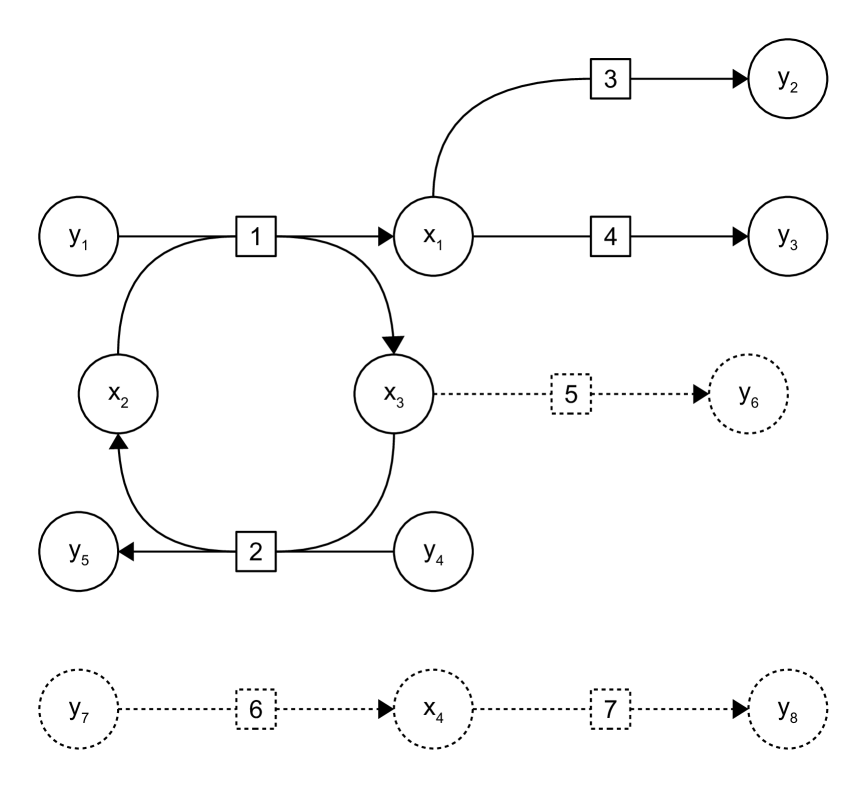
Figure 1: Diagrammatic representation of the models described in the text. The first example, containing only reactions 1 to 4, is a small metabolic pathway with a branched flux and a moiety-conserved cycle [8]. The second example extends the first through inclusion of reaction 5, which has zero flux. The third example extends the first through inclusion of reactions 6 and 7, which have constant flux. Metabolites with prefix $x$ are the variables of the models, whilst those with prefix $y$ are fixed.

parameter	value
$p_{1}$	10
$p_{2}$	10
$p_{3}$	50
$p_{4}$	10
$p_{5}$	0
$p_{6}$	1
$p_{7}$	1
$y_{1}$	10
$y_{2}$	0
$y_{3}$	0
$y_{4}$	1
$y_{5}$	1
$y_{6}$	0
$y_{7}$	1
$y_{8}$	0

Table 1: Parameter values $p$ and fixed metabolite concentrations $y$ used in the models.

parameter	value
$S_{1}$	0.056
$S_{2}$	0.769
$S_{3}$	4.231
$S_{4}$	1
$J_{1}$	3.196
$J_{2}$	3.196
$J_{3}$	2.663
$J_{4}$	0.533
$J_{5}$	0
$J_{6}$	1
$J_{7}$	1

Table 2: Steady state and initial concentrations $S$ and fluxes $J$ of the model.

Reder algorithm

In software applications such as COPASI  [11], the control matrices $C^{S}$ and $C^{J}$ are not calculated through perturbation in $e$ and calculation of a new steady state; rather the algorithm outlined by Christine Reder in 1988 is used [12], which allows calculation of the control matrices directly from the elasticities using simple matrix algebra. This algorithm is, however, only valid under certain circumstances. We step through it below to determine its validity.

We assume that $x_{0}=S$ is a steady state, perturb about this state $x=x_{0}+\tilde{x}$ and linearise.

$$\frac{dx}{dt}=\frac{d\tilde{x}}{dt}=Nv(x_{0}+\tilde{x})\approx Nv(x_{0})+N\varepsilon\tilde{x}=N\varepsilon\tilde{x}=\Delta\tilde{x},$$ (16)

as $x_{0}$ is a steady state, where $\varepsilon$ denotes the linearisation of $v$ about $x_{0}$, known as the unscaled elasticity matrix in Reder’s parlance, and $\Delta=N\varepsilon$ denotes the Jacobian of this dynamical system about $x_{0}$.

In general, the rank ${\rm r}\left(\Delta\right)=m_{0}<m$, the number of metabolites, and the system will display moiety conservations – certain metabolites can be expressed as linear combinations of other metabolites in the system [13]. Note that this number is not simply given by ${\rm r}\left(N\right)$ as is generally, erroneously, suggested.

Let $R$ denote a full set of linearly independent rows of $\Delta$ and define the link matrix $L=\Delta\Delta_{R}^{+}$, where $\Delta_{R}^{+}=\Delta_{R}^{\prime}\left(\Delta_{R}\Delta_{R}^{\prime}\right)^{-1}$ denotes the Moore-Penrose pseudoinverse [14], which may be computed using QR factorisation [15]. Thus $\Delta=L\Delta_{R}$.

Note that

$$\frac{d\tilde{x}}{dt}=\Delta\tilde{x}=L\Delta_{R}\tilde{x}=L\frac{d\tilde{x}_{R}}{dt},$$ (17)

and so we find $\tilde{x}=L\tilde{x}_{R}+T$, where the constant $T=0$.

Having developed a linear approximation of the system around the steady state, and a relationship between the independent and dependent metabolite concentrations, we now add a small perturbation $\delta$ to $e_{j}$, and calculate the change in steady state.

We have

$$\frac{d\tilde{x}_{R}}{dt} = N_{R}\,{\rm diag}\left(1+\delta_{j}\right)w(x_{0}+\tilde{x})$$ (18)

$$\approx N_{R}\,{\rm diag}\left(1+\delta_{j}\right)\left(w(x_{0})+\varepsilon\tilde{x}\right)$$ (19)

$$\approx N_{R}\varepsilon\tilde{x}+N_{R}\,{\rm diag}\left(\delta_{j}\right)w(x_{0})$$ (20)

$$= N_{R}\varepsilon\tilde{x}+\delta N_{R}v_{j}(x_{0})$$ (21)

$$= N_{R}\varepsilon L\tilde{x}_{R}+\delta N_{R}v_{j}(x_{0}),$$ (22)

where we introduce the notation $\delta_{j}$ to denote the vector with entry $\delta$ in position $j$ and 0 elsewhere, and similarly $v_{j}(x_{0})$ to denote the original steady state flux $v(x_{0})$ in position $j$ and 0 elsewhere. Thus at, steady state,

$$S=LS_{R}=-\delta L\left(N_{R}\varepsilon L\right)^{-1}N_{R}v_{j}(x_{0}).$$ (23)

Letting $\delta\to 0$, we find

$$\frac{dS}{de_{j}}=-L\left(N_{R}\varepsilon L\right)^{-1}N_{R}v_{j}(x_{0}),$$ (24)

and so the control matrices are given by

$$C^{S} = -\,{\rm diag}\left(x_{0}\right)^{-1}L\left(N_{R}\varepsilon L\right)^{-1}N_{R}\,{\rm diag}\left(v(x_{0})\right),$$ (25)

$$C^{J} = \,{\rm diag}\left(v(x_{0})\right)^{-1}\left(I-\varepsilon L\left(N_{R}\varepsilon L\right)^{-1}N_{R}\right)\,{\rm diag}\left(v(x_{0})\right).$$ (26)

These formulae allow calculation of the control matrices in terms of the local elasticities $\varepsilon$, rather than through perturbation of each $e_{j}$ and simulation. At first glance, they seem identical to those given in Reder; however, they are subtly different in the way the rows $R$ are chosen. In Reder, $R^{\ast}$ represents the linearly independent rows of the stoichiometric matrix $N$ and Reder goes on to say that her analyses are only valid if the matrix $\Delta_{R^{\ast}}=N_{R^{\ast}}\varepsilon$ is of full rank. By contrast, our method directly chooses $R$ such that $\Delta_{R}$ is of full rank. In the case ${\rm r}\left(N\right)={\rm r}\left(\Delta\right)$ (such as example one),we find $R=R^{\ast}$ and the two methods give identical results.

Example two

We create a second example where the two methods differ, extending the first model through the reaction

$$v_{5}\colon x_{3}\rightarrow y_{6},\qquad v_{5}=e_{5}p_{5}x_{3},$$ (28)

where $p_{5}=0$. Thus $v_{5}\equiv 0$ and so addition of this reaction should have no effect whatsoever on the system, and thus on other entries of the control matrices. However, the coefficients are given in COPASI (version 4.10) as

$$C^{S}_{\rm Reder}=\left(\begin{array}[]{c c c c c}-0.888&1.775&-0.878&-0.176&0\\ -2.078&2.078&-0.017&-0.003&0\\ 0&0&0&0&0\end{array}\right),$$ (29)

and the flux control coefficients

$$C^{J}_{\rm Reder}=\left(\begin{array}[]{c c c c c}-0.338&1.325&0.002&0.000&0\\ 0.284&0.716&0.002&0.000&0\\ -0.840&1.681&0.169&-0.166&0\\ -0.840&1.681&-0.831&0.833&0\\ \infty&\infty&\infty&\infty&\infty\end{array}\right).$$ (30)

These matrices are wildly different from the originals. The problem here is that addition of $v_{5}$ seems to break the conservation relationship between $x_{2}$ and $x_{3}$, at least in terms of the stoichiometric matrix. In reality, the two metabolites are still conserved. Instead choosing the independent rows as above, we find

$$C^{S}=\left(\begin{array}[]{c c c c c}0.241&0.811&-0.877&-0.175&0\\ -1.121&1.140&-0.015&-0.003&0\\ 0.204&-0.207&0.003&0.001&0\end{array}\right),$$ (31)

$$C^{J}=\left(\begin{array}[]{c c c c c}0.228&0.768&0.003&0.001&0\\ 0.228&0.768&0.003&0.001&0\\ 0.228&0.768&0.170&-0.166&0\\ 0.228&0.768&-0.830&0.834&0\\ 0&0&0&0&1\end{array}\right).$$ (32)

We see that, as expected, the upper-left portions of each matrix are unaffected by the addition of the null reaction $v_{5}$. Moreover, each matrix still satisfies the summation theorems.

Example three

For a final example model, we add (to the original model) reactions

$$v_{6}\colon x_{7}\rightarrow x_{4},\qquad v_{6}=e_{6}p_{6}y_{7},$$ (33)

$$v_{7}\colon x_{4}\rightarrow y_{9},\qquad v_{7}=e_{7}p_{7}.$$ (34)

These reactions have constant rate, but are disconnected and independent of the rest of the system. Here the result of COPASI is worse than before, with $C^{S}$ and $C^{J}$ undefined (containing only NaN entries). We can have some sympathy here, as any perturbation in $e_{6}$ or $e_{7}$ leads to no steady state for $x_{4}$. However, the other entries for the matrix should be unaffected. Choosing $R$ differently, as above, we find the more appealing solutions:

$$C^{S}=\left(\begin{array}[]{c c c c c c}0.241&0.811&-0.877&-0.175&0&0\\ -1.121&1.140&-0.015&-0.003&0&0\\ 0.204&-0.207&0.003&0.001&0&0\end{array}\right),$$ (35)

$$C^{J}=\left(\begin{array}[]{c c c c c c}0.228&0.768&0.003&0.001&0&0\\ 0.228&0.768&0.003&0.001&0&0\\ 0.228&0.768&0.170&-0.166&0&0\\ 0.228&0.768&-0.830&0.834&0&0\\ 0&0&0&0&1&0\\ 0&0&0&0&0&1\\ \end{array}\right).$$ (36)

Summary

The existing method for calculating metabolic control matrices, though widely used, is only valid for certain models. The key issue is that dynamics, as well as stoichiometry, must be taken into account when determining moiety conservation. However, this small modification will ensure that the algorithm may be applied in all cases.

Supplementary material

The models described above are available in SBML format [16] from the BioModels Database [17]. Their accession numbers are:

• model 1: biomodels.db:MODEL1305030000

• model 2: biomodels.db:MODEL1305030001

• model 3: biomodels.db:MODEL1305030002

Acknowledgements

I am grateful for the financial support of the EU FP7 (KBBE) grant 289434 “BioPreDyn: New Bioinformatics Methods and Tools for Data-Driven Predictive Dynamic Modelling in Biotechnological Applications”. Thanks to Mark Muldoon for innumerable discussions, and to Pedro Mendes for access to his innumerable library. Thanks also to Stefan Hoops for spotting a typo in the original version.

References

- [1] Kacser H, Burns JA (1973) The control of flux. Symp Soc Exp Biol 27:65–104.
- [2] Kacser H, Burns JA, Fell DA (1995) The control of flux: 21 years on. Biochem Soc Trans 23:341–366.
- [3] Heinrich R, Rapoport TA (1974) A linear steady-state treatment of enzymatic chains. General properties, control and effector strength. Eur J Biochem 42:89–95. doi:10.1111/j.1432-1033.1974.tb03318.x
- [4] Fell DA (1992) Metabolic control analysis: a survey of its theoretical and experimental development. Biochem J 286:313–330.
- [5] Fell DA (1996) Understanding the control of metabolism. Portland Press. isbn:1-85578-047-X
- [6] Heinrich R, Schuster S (1996) The regulation of cellular systems. Chapman & Hall. isbn:0-412-03261-9
- [7] Ingalls BP, Sauro HM (2003) Sensitivity analysis of stoichiometric networks: an extension of metabolic control analysis to non-steady state trajectories. J Theor Biol 222:23–36. doi:10.1016/S0022-5193(03)00011-0
- [8] Hofmeyr JS, Cornish-Bowden A (1996) Co-response analysis: a new experimental strategy for metabolic control analysis. J Theor Biol 182:371–380. doi:10.1006/jtbi.1996.0176 biomodels.db:MODEL1304300000
- [9] Greenberg JL (1995) The Problem of the Earth’s Shape from Newton to Clairaut. Cambridge University Press. isbn:0-521-38541-5
- [10] Giersch C (1988) Control analysis of metabolic networks. 1. Homogeneous functions and the summation theorems for control coefficients. Eur J Biochem 174:509–513. doi:10.1111/j.1432-1033.1988.tb14128.x
- [11] Hoops S, Sahle S, Gauges R, Lee C, Pahle J, Simus N, Singhal M, Xu L, Mendes P, Kummer U (2006) COPASI: a COmplex PAthway SImulator. Bioinformatics 2006 22:3067–3074. doi:10.1093/bioinformatics/btl485
- [12] Reder CA (1988) Metabolic control theory: a structural approach. J Theor Biol 135:175–201. doi:10.1016/S0022-5193(88)80073-0
- [13] Smallbone K, Simeonidis E, Swainston N, Mendes P (2010) Towards a genome-scale kinetic model of cellular metabolism. BMC Syst Biol 4:6. doi:10.1186/1752-0509-4-6
- [14] Penrose R (1955) A generalized inverse for matrices. Math Proc Cambridge 3:406–413. doi:10.1017/S0305004100030401
- [15] Sauro HM, Ingalls B (2004) Conservation analysis in biochemical networks: computational issues for software writers. Biophys Chem 109:1–15. doi:10.1016/j.bpc.2003.08.009
- [16] Hucka M, Finney A, Sauro HM, Bolouri H, Doyle JC, Kitano H, Arkin AP, Bornstein BJ, Bray D, Cornish-Bowden A, Cuellar AA, Dronov S, Gilles ED, Ginkel M, Gor V, Goryanin II, Hedley WJ, Hodgman TC, Hofmeyr JH, Hunter PJ, Juty NS, Kasberger JL, Kremling A, Kummer U, Le Novère N, Loew LM, Lucio D, Mendes P, Minch E, Mjolsness ED, Nakayama Y, Nelson MR, Nielsen PF, Sakurada T, Schaff JC, Shapiro BE, Shimizu TS, Spence HD, Stelling J, Takahashi K, Tomita M, Wagner J, Wang J, SBML Forum (2003) The systems biology markup language (SBML): a medium for representation and exchange of biochemical network models. Bioinformatics 19:524–531. doi:10.1093/bioinformatics/btg015
- [17] Li C, Donizelli M, Rodriguez N, Dharuri H, Endler L, Chelliah V, Li L, He E, Henry A, Stefan MI, Snoep JL, Hucka M, Le Novère N, Laibe C (2010) BioModels Database: An enhanced, curated and annotated resource for published quantitative kinetic models. BMC Syst Biol 4:92. doi:10.1186/1752-0509-4-92