Quantum Fluctuation Driven First-order Phase Transitions In Optical Lattices

Abstract

We study quantum fluctuation driven first-order phase transitions of a two-species bosonic system in a three-dimensional optical lattice. Using effective potential method we find that the superfluid-Mott insulator phase transition of one type of bosons can be changed from second-order to first-order by the quantum fluctuations of the other type of bosons. The study of the scaling behaviors near the quantum critical point shows that the first-order phase transition has a different universality from the second-order one. We also discuss the observation of this phenomenon in the realistic cold-atom experiments based on the in situ density measurements.

I Introduction

Recently, the researches of quantum criticality in cold-atom systems have attracted a great deal of interest. Several schemes have been proposed to determine the critical properties by extracting the universal scaling functions from the atomic density profiles Zhou ; Hazzard ; Zhang . The experimental observations of quantum critical behaviors of ultracold atoms have also been reported Donner ; Zhang1 . As a clean and highly controllable system, cold atoms can be a good play ground to study various quantum critical behaviors.

An intriguing phenomenon near the quantum critical points (QCPs) is the effect of quantum fluctuation driven first-order phase transitions. The QCPs may become unstable in the appearance of competing orders. The nature of the phase transition can be changed from second- to first-order by the quantum fluctuations. This phenomenon was first discussed by S. Coleman and E. Weinberg Coleman . They investigated a theory of a massless charged meson coupled to the electrodynamic field using effective potential method. Starting from a model without symmetry breaking at tree level they found that the one-loop effective potential indicated a new energy minimum appearing away from the origin. Independently, Halperin, Lubensky, and Ma Halperin discovered the same phenomenon in the Ginzburg-Landau theory of superconductor to normal metal transition and showed that the fluctuations of the electromagnetic field induce a first-order transition. Quantum fluctuation driven first-order phase transitions were also discussed in systems with multiple coupling constants Amit ; Domb . Recently, there have appeared more examples of the nature of the quantum phase transition is predicted to become discontinuous as the QCP is approached Continentino ; Ferreira ; Yang ; Qi ; Millis ; She ; Diehl ; Bonnes .

In this letter we investigate the quantum fluctuation driven first-order phase transitions of a two-species boson system in a three dimensional optical lattice. This phenomenon has not been sufficiently explored in condensed matter physics. With the recent progress in the researches of the quantum critical behaviors in cold atom physics we are able to observe this phenomenon in a realistic experiment. Multi-component bosonic systems have been studied both experimentally Catani ; Trotzky ; Thalhammer ; Gadway and theoretically Han ; Buonsante ; Chen ; Isacsson ; Li ; Altman ; Kuklov ; Kuklov2 . Compared with the paradigmatic superfluid to Mott insulator transition of a single component Bose gas in an optical lattice Fisher ; Jaksch ; Greiner ; Stoferle ; Spielman , multi-component bosonic systems have much richer phase diagrams. In our work we implement Coleman and Weinberg’s effective potential method Coleman to calculate the quantum corrections to the classical action up to one-loop level. We find that the superfluid-Mott insulator phase transition of one type of bosons can be driven from second-order to first-order by the quantum fluctuations of the other type. We study the scaling behaviors near the first-order phase transition and give a feasible proposal to observe this phenomenon in cold-atom experiments.

II Two-species Bose-Hubbard model

To describe Bose-Bose mixtures loaded into optical lattices, we consider the following two-species Bose-Hubbard Hamiltonian,

$$H= -\sum_{\alpha,<ij>}t_{\alpha}(\hat{b}^{\dagger}_{\alpha i}\hat{b}_{\alpha j}+\hat{b}^{\dagger}_{\alpha j}\hat{b}_{\alpha i})-\sum_{\alpha,i}\mu_{\alpha}\hat{n}_{\alpha i}$$ (2)

$$+\sum_{\alpha,i}\frac{U_{\alpha}}{2}\hat{n}_{\alpha i}(\hat{n}_{\alpha i}-1)+U_{AB}\sum^{N}_{i=1}\hat{n}_{1i}\hat{n}_{2i}.$$

Here $b^{\dagger}_{\alpha i}$ creates a boson of sort $\alpha=A,B$ at site $i$. The first term in the Hamiltionian represents the hopping of bosons of types $A$ and $B$ between the nearest-neighbor pairs of sites $<ij>$ with hopping amplitudes $t_{A}$ and $t_{B}$. $\hat{n}_{\alpha i}\equiv\hat{b}^{\dagger}_{\alpha i}\hat{b}_{\alpha i}$ is the number operator of the $\alpha$ type boson at the site $i$. We have two chemical potential $\mu_{A}$ and $\mu_{B}$ to fix the total number of type $A$ and $B$ bosons. $U_{\alpha}$ and $U_{AB}$ denote the intra- and inter-species on-site interaction strengthes.

The mean-field analysis shows that the system has three different phases Chen : (I) both species A and B stay in the superfluid phases; (II) one species is in the superfluid phase and the other one is in the Mott insulator phase; and (III) both species are in the Mott insulator phases. Two examples of the phase diagrams are shown in Fig. 1.

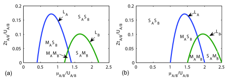
Figure 1: (Color online) The phase diagrams of the two-species Bose-Hubbard model. The axes are either $Zt_{A}$ versus $\mu_{A}$ or $Zt_{B}$ versus $\mu_{B}$ , all in units of $U_{A}$ or $U_{B}$, where $Z$ is the number of the nearest neighbors around each lattice point. Curves $L_{A}$ and $L_{B}$ denote the superfluid-Mott insulator phase boundaries for species A and B. Depending on different parameters, $L_{A}$ and $L_{B}$ may divide the diagram into two, three, or four regions, two examples are presented here: (a)$n^{0}_{1}=1$, $n^{0}_{2}=2$ and $U_{AB}/U_{A}=U_{AB}/U_{B}=0.5$; (b)$n^{0}_{1}=1$, $n^{0}_{2}=2$ and $U_{AB}/U_{A}=U_{AB}/U_{B}=0.2$. Labels “$S_{A}S_{B}$”, “$M_{A}M_{B}$”, “$S_{A}M_{B}$” and “$M_{A}S_{B}$” denote for superfluid phase for both species A and B, Mott insulator phase for both species A and B, superfluid phase for species A Mott insulator phase for species B and superfluid phase for species B Mott insulator phase for species A.

To study the quantum fluctuation effects in the vicinity of QCPs we may take the limit of vanishing lattice constant and finally write down a continuum quantum field theory to describe the phase transitions. This can be done by following a standard procedure Sachdev : (I) writing the partition function in the coherent state path integral representation; (II) decoupling the hoping terms by introducing two auxiliary fields $\varphi_{1}$ and $\varphi_{2}$ through the Hubbard-Stratanovich transformation; and (III) integrating out the fields $b_{Ai}^{\dagger}$, $b_{Ai}$, $b_{Bi}^{\dagger}$ and $b_{Bi}$. Then the action can be written as

$$S= \int d\tau d^{d}x\big{\{}u_{1}\varphi_{1}^{\ast}\partial_{\tau}\varphi_{1}+v_{1}|\partial_{\tau}\varphi_{1}|^{2}+w_{1}|\nabla\varphi_{1}|^{2}$$ (5)

$$+u_{2}\varphi_{2}^{\ast}\partial_{\tau}\varphi_{2}+v_{2}|\partial_{\tau}\varphi_{2}|^{2}+w_{2}|\nabla\varphi_{2}|^{2}+r_{1}|\varphi_{1}|^{2}$$

$$+r_{2}|\varphi_{2}|^{2}+\frac{g_{1}}{2}|\varphi_{1}|^{4}+\frac{g_{2}}{2}|\varphi_{2}|^{4}+g_{3}|\varphi_{1}|^{2}|\varphi_{2}|^{2}\big{\}}.$$

The average of the two Hubbard-Stratanovich field $\varphi_{1}$ and $\varphi_{2}$ are proportional to $\langle b_{A}(x,\tau)\rangle$ and $\langle b_{B}(x,\tau)\rangle$. Hence, they can be taken as the superfluid order parameters. All the coefficients in Eq.(5) can be expressed in terms of the hopping amplitudes $t_{\alpha}$, the chemical potentials $\mu_{\alpha}$ and the on-site interaction strengths $U_{\alpha}$ and $U_{AB}$.

$$r_{1} =\frac{1}{zt_{A}}-\frac{n^{0}_{A}+1}{\Delta_{A+}}-\frac{n^{0}_{A}}{\Delta_{A-}},$$ (6)

$$r_{2} =\frac{1}{zt_{B}}-\frac{n^{0}_{B}+1}{\Delta_{B+}}-\frac{n^{0}_{B}}{\Delta_{A-}},$$ (7)

where

$$\Delta_{A(B)+}=-\mu_{A(B)}+U_{A(B)}n^{0}_{A(B)}+U_{AB}n^{0}_{B(A)},$$ (8)

$$\Delta_{A(B)-}=\mu_{A(B)}-U_{A(B)}(n^{0}_{A(B)}-1)-U_{AB}n^{0}_{B(A)},$$ (9)

which denote the particle and hole excitation energy of the species $A(B)$. The occupation numbers $n^{0}_{A(B)}$ is defined as the smallest integer larger than $\frac{U_{AB}(U_{AB}-U_{B(A)}-2\mu_{B(A)})+2\mu_{A(B)}U_{B(A)}}{2(U_{A(B)}U_{B(A)}-U^{2}_{AB})}$. The equation $r_{1}=0$ and $r_{2}=0$ generate the mean-field phase boundaries in Fig. 1. Furthermore, the two-species Bose-Hubbard model obeys a $U(1)\times U(1)$ gauge symmetry, which implies that the model is invariant under the transformation $b_{\alpha}(\tau)\rightarrow b_{\alpha}(\tau)e^{i\theta_{\alpha}(\tau)}$, $\phi_{\alpha}(\tau)\rightarrow\phi_{\alpha}(\tau)e^{i\theta_{\alpha}(\tau)}$ and $\mu_{\alpha}\rightarrow\mu_{\alpha}+i\partial_{\tau}\theta_{\alpha}(\tau)$, where $\alpha=A,B$. This gauge invariance helps to fix the coefficients of the first- and second-order time derivatives as Sachdev $u_{1}=-\frac{1}{t_{A}^{2}}\frac{\partial t_{A}}{\partial\mu_{A}}$, $u_{2}=-\frac{1}{t_{B}^{2}}\frac{\partial t_{B}}{\partial\mu_{B}}$, $v_{1}=\frac{1}{t_{A}^{3}}(\frac{\partial t_{A}}{\partial\mu_{A}})^{2}-\frac{1}{2t_{A}^{2}}\frac{\partial^{2}t_{A}}{\partial\mu_{A}^{2}}$ and $v_{2}=\frac{1}{t_{B}^{3}}(\frac{\partial t_{B}}{\partial\mu_{B}})^{2}-\frac{1}{2t_{B}^{2}}\frac{\partial^{2}t_{B}}{\partial\mu_{B}^{2}}$, where partial derivatives $\partial t_{A(B)}/\partial\mu_{A(B)}$ and $\partial^{2}t_{A(B)}/\partial\mu_{A(B)}^{2}$ can be calculated from Eq. (7) for fixed $r_{i}$. Along the mean-field phase boundaries the parameter $u_{1}$ and $u_{2}$ can be expressed as

$$u_{1} =\frac{z(n^{0}_{A}+1)}{\Delta_{A+}^{2}}-\frac{zn^{0}_{A}}{\Delta_{A-}^{2}},$$ (10)

$$u_{2} =\frac{z(n^{0}_{B}+1)}{\Delta_{B+}^{2}}-\frac{zn^{0}_{B}}{\Delta_{B-}^{2}}.$$ (11)

It’s straight forward to see that at the tips of the insulating lobes coefficients $u_{1}$ and $u_{2}$ vanish. For simplicity we consider the QCPs at the tips of the insulating lobes, then he action of Eq. (5) is deduced to a relativistic theory. This also reflects the particle-hole symmetry at the tips of the insulating lobes. For example, we take the insulating lobes of $n^{0}_{A}=n^{0}_{B}=1$. Using Eq. (11) we obtain

$$\mu_{A}(\mu_{B})=U_{A}(U_{B})/(\sqrt{2}+1)+U_{AB},$$ (12)

for $u_{1}=u_{2}=0$. With this relations we can fine-tune the system around the tips of the lobes. In the harmonic trap this condition locates a shell in the cloud of gas. By varying the the optical potential depth we will be able to change the hopping term $t_{\alpha}$ so that the system can go across the phase transition point. Furthermore, the interaction couplings can also be calculated as

$$g_{1}=$$ (13)

$$\frac{2(n^{(0)}_{A}+1)^{2}}{\Delta_{A+}^{3}}+\frac{2(n^{(0)}_{A})^{2}}{\Delta_{A-}^{3}}+\frac{(n^{(0)}_{A}+1)n^{(0)}_{A}}{\Delta_{A+}\Delta_{A-}}(\frac{1}{\Delta_{A+}}+\frac{1}{\Delta_{A-}}),$$ (14)

$$g_{2}=$$ (15)

$$\frac{2(n^{(0)}_{B}+1)^{2}}{\Delta_{B+}^{3}}+\frac{2(n^{(0)}_{B})^{2}}{\Delta_{B-}^{3}}+\frac{(n^{(0)}_{B}+1)n^{(0)}_{B}}{\Delta_{B+}\Delta_{B-}}(\frac{1}{\Delta_{B+}}+\frac{1}{\Delta_{B-}}),$$ (16)

$$g_{3}=\frac{(n^{(0)}_{A}+1)(n^{(0)}_{B}+1)}{\Delta_{A+}\Delta_{B+}}(\frac{1}{\Delta_{A+}}+\frac{1}{\Delta_{B+}})$$ (17)

$$+\frac{n^{(0)}_{A}n^{(0)}_{B}}{\Delta_{A-}\Delta_{B-}}(\frac{1}{\Delta_{A-}}+\frac{1}{\Delta_{B-}})$$ (18)

$$+\frac{(n^{(0)}_{A}+1)n^{(0)}_{B}}{\Delta_{A+}\Delta_{B-}}(\frac{1}{\Delta_{A+}}+\frac{1}{\Delta_{B-}})$$ (19)

$$+\frac{(n^{(0)}_{B}+1)n^{(0)}_{A}}{\Delta_{A-}\Delta_{B+}}(\frac{1}{\Delta_{A-}}+\frac{1}{\Delta_{B+}}).$$ (20)

In above equations we ignore the processes of two-particle or two-hole excitations of one species since the one-particle and one-hole excitation are dominant.

III The Coleman-Weinberg effective potential

At the tips of the insulating lobes the classical potential of this theory is posed right on the edge of the symmetry breaking, that is $r_{1}=r_{2}=0$ in Eq. (5). We wonder whether the quantum fluctuations will break the symmetry or not. To answer this question we implement the Weinberg and Coleman’s effective potential method Coleman to calculate the quantum corrections to the action of Eq. (5).

The notion of the effective potential has been found to be very useful in theories exhibiting spontaneously broken symmetry. It allows one to calculate quantum corrections to the classical picture of spontaneous symmetry breaking. This method is often useful in the case with the presence of a classical external field. For instance, a theory with a mean-field and quantum fluctuations. The effective potential method was first developed in High energy physics Coleman . However, it’s also widely used in condensed matter theories. Basically, we expand the field in terms of its mean value and quantum fluctuations. Then we can integrate out the quantum fluctuations to obtain an effective theory of the mean field. All the quantum properties are incorporated in this effective theory. The nature of the effective potential can be totally different from the classical one. For example, the phase transition can be changed from second order to first order Continentino ; Ferreira ; Yang ; Qi ; Millis ; She ; Diehl ; Bonnes .

To obtain the effective potential we expand the fields $\varphi_{1}$ and $\varphi_{2}$ in Eq. (5) in terms of their mean fields and quantum fluctuations $\varphi_{1}\rightarrow\phi_{1}+\delta\phi_{1}$ and $\varphi_{2}\rightarrow\phi_{2}+\delta\phi_{2}$ and keep the fluctuation up to the second order. Then the action can be written as

$$S[\phi_{1},\phi_{2}]=S_{0}[\phi_{1},\phi_{2}]+\frac{1}{2}\int d\tau d^{3}x\delta\Phi^{\dagger}{\mathcal{G}}^{-1}\delta\Phi,$$ (21)

where $S_{0}[\phi_{1},\phi_{2}]=\int d\tau d^{3}x\{|\partial_{\tau}\phi_{1}|^{2}+|\nabla\phi_{1}|^{2}+|\partial_{\tau}\phi_{2}|^{2}+|\nabla\phi_{2}|^{2}+\frac{g_{1}}{2}|\phi_{1}|^{4}+\frac{g_{2}}{2}|\phi_{2}|^{4}+g_{3}|\phi_{1}|^{2}|\phi_{2}|^{2}\}$. The parameters $v_{1}$, $w_{1}$, $v_{2}$ and $w_{2}$ have been absorbed into the coordinates. Field $\delta\Phi^{\dagger}=[\delta\phi_{1}^{\ast},\delta\phi_{1},\delta\phi_{2}^{\ast},\delta\phi_{2}]$ and $\delta\Phi$ is its Hermitian conjugate. The matrix $\mathcal{G}^{-1}$ is

$$\left(\begin{array}[]{cccc}-\partial^{2}+2g_{1}\phi_{1}^{\ast}\phi_{1}+g_{3}\phi_{2}^{\ast}\phi_{2}&g_{1}\phi_{1}\phi_{1}&g_{3}\phi_{1}\phi_{2}^{\ast}&g_{3}\phi_{1}\phi_{2}\\ g_{1}\phi_{1}^{\ast}\phi_{1}^{\ast}&-\partial^{2}+2g_{1}\phi_{1}^{\ast}\phi_{1}+g_{3}\phi_{2}^{\ast}\phi_{2}&g_{3}\phi_{1}^{\ast}\phi_{2}^{\ast}&g_{3}\phi_{1}^{\ast}\phi_{2}\\ g_{3}\phi_{1}^{\ast}\phi_{2}&g_{3}\phi_{1}\phi_{2}&-\partial^{2}+2g_{2}\phi_{2}^{\ast}\phi_{2}+g_{3}\phi_{1}^{\ast}\phi_{1}&g_{2}\phi_{2}\phi_{2}\\ g_{3}\phi_{1}^{\ast}\phi_{2}^{\ast}&g_{3}\phi_{1}\phi_{2}^{\ast}&g_{2}\phi_{2}^{\ast}\phi_{2}^{\ast}&-\partial^{2}+2g_{2}\phi_{2}^{\ast}\phi_{2}+g_{3}\phi_{1}^{\ast}\phi_{1}\end{array}\right),$$ (26)

where $\partial^{2}=\partial_{\tau}^{2}+\nabla^{2}$.

After we integrate out the fluctuation fields $\delta\Phi$ the effective potential of our action up to one-loop level can be calculated as

$$V_{\rm eff}=g_{1}/2(\phi^{\ast}_{1}\phi_{1})^{2}+g_{2}/2(\phi^{\ast}_{2}\phi_{2})^{2}+g_{3}\phi^{\ast}_{1}\phi_{1}\phi^{\ast}_{2}\phi_{2}$$ (27)

$$+\frac{1}{64\pi^{2}}\big{\{}m_{1}^{4}\ln m^{2}_{1}+m_{2}^{4}\ln m^{2}_{2}+m_{+}^{4}\ln m^{2}_{+}+m_{-}^{4}\ln m^{2}_{-}\big{\}}$$ (28)

$$+B_{1}|\phi_{1}|^{2}+B_{2}|\phi_{2}|^{2}+C_{1}|\phi_{1}|^{4}+C_{2}|\phi_{2}|^{4}+C_{3}|\phi_{1}|^{2}|\phi_{2}|^{2},$$ (29)

(30)

where

$$m_{1}^{2}=g_{1}|\phi_{1}|^{2}+g_{3}|\phi_{2}|^{2},$$ (31)

$$m_{2}^{2}=g_{2}|\phi_{2}|^{2}+g_{3}|\phi_{1}|^{2},$$ (32)

$$m^{2}_{\pm}=\frac{1}{2}\big{|}(3g_{1}+g_{3})|\phi_{1}|^{2}+(3g_{2}+g_{3})|\phi_{2}|^{2}$$ (33)

$$\pm\sqrt{[(3g_{1}-g_{3})|\phi_{1}|^{2}-(3g_{2}-g_{3})|\phi_{2}|^{2}]^{2}+16g^{2}_{3}|\phi_{1}|^{2}|\phi_{2}|^{2}}\big{|}.$$ (34)

The terms with coefficients $B_{1}$, $B_{2}$, $C_{1}$, $C_{2}$ and $C_{3}$ in Eq. (30) are the renormalization counterterms. They can be fixed by imposing the renormalization conditions $\frac{\partial V_{\rm eff}}{\partial\phi_{1}^{\ast}\partial\phi_{1}}\big{|}_{\phi_{1}=0,\phi_{2}=0}=0$, $\frac{\partial V_{\rm eff}}{\partial\phi_{2}^{\ast}\partial\phi_{2}}\big{|}_{\phi_{1}=0,\phi_{2}=0}=0$, $V_{\rm eff}(|\phi_{1}|=M,|\phi_{2}|=0)=\frac{g_{1}}{2}M^{4}$, $V_{\rm eff}(|\phi_{1}|=0,|\phi_{2}|=M)=\frac{g_{2}}{2}M^{4}$, $V_{\rm eff}(|\phi_{1}|=M,|\phi_{2}|=M)=(\frac{g_{1}}{2}+\frac{g_{2}}{2}+g_{3})M^{4}$, where $M$ is the renormalization parameter and can be chosen arbitrarily.

The minima of the effective potential actually give the true vacuum states with the quantum fluctuation corrections. Compared with the classical potential where the vacuum is right at the origin, the one-loop effective potential in Eq. (30) exhibits new vacua away from the origin. This can be shown in the three-dimensional and contour plots of the effective potential in Fig. 2. Without loss of generality we already simplified the effective potential by fixing the complex fields to their real directions so that the effective potential can be easily visualized in Fig. 2. That is, we take $\phi_{1}\rightarrow\phi_{1R}$ and $\phi_{2}\rightarrow\phi_{2R}$. $\phi_{1R}$ and $\phi_{2R}$ are real fields.

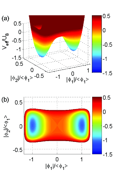
Figure 2: (Color online) The three-dimensional and contour plots of the effective potential of the two species Bose-Hubbard model. Coefficients $r_{1}=r_{2}=0$ for both graph (a) and (b). We use $U_{B}$ as the energy scale to make all the couplings dimensionless. Here we take $U_{B}/U_{A}=0.3$, then the interaction couplings are $g_{2}U_{B}^{3}=101.9$ and $g_{3}U_{B}^{3}=26.5$. We take renormalization parameter $M=<\phi_{1}>$, where $<\phi_{1}>$ is the vacuum of field $\phi_{1}$. The interaction coupling $g_{1}$ is eliminated by the condition $\frac{\partial V_{\rm eff}}{\partial\phi_{1}}|_{|\phi_{1}|=<\phi_{1}>}=0$.

Here we take the parameters $g_{1}<g_{2}$ in different values then we observe that the new vacua appear at $\phi^{\ast}_{1}\phi_{1}\neq 0,~{}\phi^{\ast}_{2}\phi_{2}=0$ in Fig. 2 (a) and (b). Hence, the $U(1)\times U(1)$ symmetry is spontaneously broken to $U(1)$ symmetry. At the new vacuum the field $\phi_{2}$ stays in the insulator phase and field $\phi_{1}$ is in the superfluid phase. Notice that in Fig. 2 we choose renormalization parameter $M=<\phi_{1}>$ since $M$ is arbitrary, where $<\phi_{1}>$ is the vacuum of field $\phi_{1}$. By setting $M=<\phi_{1}>$ the interaction coupling $g_{1}$ is eliminated through the condition $\frac{\partial V_{\rm eff}}{\partial\phi_{1}}|_{|\phi_{1}|=<\phi_{1}>}=0$. Here we introduce a dimensional parameter $<\phi_{1}>$ and eliminate a dimensionless one $g_{1}$. This is called the dimensional transmutation Coleman .

However, the appearance of new vacua can be an artifact since the new vacua may lie outside the range of validity of the one-loop approximation Coleman . In order to investigate the validity of our result we take the direction of $\phi^{\ast}_{2}\phi_{2}=0$ in the effective potential to explore the vacuum. Along this direction the effective potential can be reduced to

$$V_{\rm eff}= g_{1}/2(\phi^{\ast}_{1}\phi_{1})^{2}+\frac{1}{32\pi^{2}}g^{2}_{3}(\phi^{\ast}_{1}\phi_{1})^{2}\ln\frac{\phi^{\ast}_{1}\phi_{1}}{M^{2}}.$$ (36)

The effective potential of Eq. (36) includes a term of $\ln\frac{\phi^{\ast}_{1}\phi_{1}}{M^{2}}$. The logarithm of a small number is negative. Hence, the minimum arose from balancing a term of order $g_{1}$ against a term of order $g^{2}_{3}\ln\frac{\phi^{\ast}_{1}\phi_{1}}{M^{2}}$. Even though the second term formally arises in a higher order of our expansion, there is no reason why $g_{1}$ can not be of the same order of magnitude as $g_{3}^{2}$. In the realistic system the coupling constant $g_{1}$ and $g_{3}$ can be calculated though Eq. (20). With the condition Eq. (12) we can derive the couplings approximately as $g_{1}\sim\frac{1}{U_{A}^{3}}$ and $g_{3}\sim\frac{1}{U_{A}U_{B}}(\frac{1}{U_{A}}+\frac{1}{U_{B}})$. If we tune $U_{A}\gg U_{B}$ we can have $g_{3}^{2}\gg g_{1}$. Hence, our result is inside the range of validity of the one-loop approximation. The new vacuum is illustrated in Fig. 3. As $g_{3}$ gets stronger the vacuum becomes deeper.

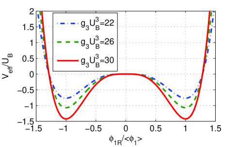
Figure 3: (Color online) The effective potential along the $\phi^{\ast}_{2}\phi_{2}=0$ direction with different values of $g_{3}$. The parameters are $r_{1}=r_{2}=0$ and $g_{2}U_{B}^{3}=101.9$. $g_{3}$ is indicated in the graph. We take renormalization parameter $M=<\phi_{1}>$. The interaction coupling $g_{1}$ is eliminated by the condition $\frac{\partial V_{\rm eff}}{\partial\phi_{1}}|_{|\phi_{1}|=<\phi_{1}>}=0$.

The excitation spectrum around the new vacuum can be calculated by expanding the effective action around the new vacuum of $|\phi_{1}|^{2}=\rho,~{}~{}|\phi_{2}|^{2}=0$. Let us write $\phi_{1}\rightarrow\sqrt{\rho}+\delta\phi_{1},~{}~{}~{}~{}\phi_{2}\rightarrow\delta\phi_{2}$. Up to the quadratic order of the fields $\delta\phi_{1}$ and $\delta\phi_{2}$ a straight forward computation yields $S=\int d\tau d^{3}x\big{\{}|\partial_{\tau}\delta\phi_{1}|^{2}+|\nabla\delta\phi_{1}|^{2}+|\partial_{\tau}\delta\phi_{2}|^{2}+|\nabla\delta\phi_{2}|^{2}-\frac{g_{3}^{2}}{64\pi^{2}}\rho^{2}+\frac{g_{3}^{2}}{32\pi^{2}}\rho(\delta\phi_{1}^{2}+\delta\phi^{\ast 2}_{1}+2\delta\phi_{1}^{\ast}\delta\phi_{1})+g_{3}\rho\delta\phi^{\ast}_{2}\delta\phi_{2}\big{\}}.$ The diagonalization of the mass term of field $\delta\phi_{1}$ generates two mass eigenvalues $m_{1}^{2}=\frac{g_{3}^{2}}{16\pi^{2}}\rho$ or $0$. The massless excitation is the Goldstone mode, which indicates the break down of $U(1)$ symmetry of field $\phi_{1}$. The field $\delta\phi_{2}$ has two modes with the same mass $m_{2}^{2}=g_{3}\rho$.

IV Nature of the phase transition

We investigate the effective potential with non-zero parameter $r_{1}$ and $r_{2}$. For large enough $r_{1}$ and $r_{2}$ the vacuum of the effective potential is at the origin. Now we vary the coefficient $r_{1}$ to study how the vacuum changes. Along the direction of $\phi^{\ast}_{2}\phi_{2}=0$ the effective potential is obtained as $V_{\rm eff}=r_{1}|\phi_{1}|^{2}+\frac{g_{1}}{2}|\phi_{1}|^{4}+\frac{(r_{2}+g_{3}|\phi_{1}|^{2})^{2}}{32\pi^{2}}\ln(r_{2}+g_{3}|\phi_{1}|^{2})-\frac{r^{2}_{2}\ln r_{2}}{32\pi^{2}}-\frac{(\phi^{\ast}_{1}\phi_{1})^{2}}{32\pi^{2}M^{4}}(r_{2}+g_{3}M^{2})^{2}\ln(r_{2}+g_{3}M^{2}).$ Here if we choose the value of $r_{1}$ small enough a local minimum will appear away from the origin as show in Fig. 4 (a). For simplicity we take the renormalization parameter $M^{2}=\langle\phi_{1}\rangle^{2}$ , where $\langle\phi_{1}\rangle$ is the average value of the field $\phi_{1}$ at the local minimum. Using the condition of $\frac{\partial V_{\rm eff}}{\partial\phi_{1}}|_{\phi_{1}^{\ast}\phi_{1}=\langle\phi_{1}\rangle^{2}}=0$ the the effective potential can be simplified as

$$V_{\rm eff}=r_{1}|\phi_{1}|^{2}+\frac{(r_{2}+g_{3}|\phi_{1}|^{2})^{2}}{32\pi^{2}}\ln(r_{2}+g_{3}|\phi_{1}|^{2})$$ (37)

$$+\frac{(\phi^{\ast}_{1}\phi_{1})^{2}}{2\langle\phi_{1}\rangle^{2}}\Big{(}-r_{1}-\frac{g_{3}(r_{2}+g_{3}\langle\phi_{1}\rangle^{2})}{16\pi^{2}}\ln(r_{2}+g_{3}\langle\phi_{1}\rangle^{2})$$ (38)

$$-\frac{g_{3}}{32\pi^{2}}(r_{2}+g_{3}\langle\phi_{1}\rangle^{2})\Big{)}-\frac{r^{2}_{2}\ln r_{2}}{32\pi^{2}}.$$ (39)

As we lower the parameter $r_{1}$ the vacuum of above effective potential jumps from the origin to a new vacuum at $\phi_{1}^{\ast}\phi_{1}=\langle\phi_{1}\rangle^{2}$ and $\phi_{2}^{\ast}\phi_{2}=0$, where the type A bosons become superfluid and type B bosons stay in the insulator phase. This phase transition occurs at a finite value of $r_{1}$. The change of the vacuum is shown in graph (a) of Fig. 4.

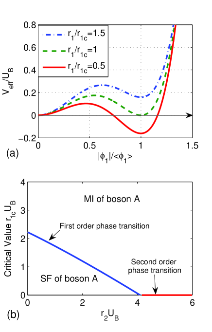
Figure 4: (Color online) (a) The effective potential along the $\phi^{\ast}_{2}\phi_{2}=0$ direction with different values of $r_{1}$, where $r_{2}U_{B}=3$, $g_{2}U_{B}^{3}=101.9$, $g_{3}U_{B}^{3}=26.5$ and $r_{1c}U_{B}\simeq 0.64$. (b) The critical value $r_{1c}$ of the first-order phase transition of type A bosons as a function of coefficient $r_{2}$.

As $r_{1}$ approaches to the critical value $r_{1c}$ there is a first-order phase transition, where critical value of $r_{1}$ is

$$r_{1c}=\frac{1}{16\pi^{2}\langle\phi_{1}\rangle^{2}}r^{2}_{2}\ln r_{2}+\frac{g_{3}}{32\pi^{2}}(r_{2}+g_{3}\langle\phi_{1}\rangle^{2})$$ (40)

$$-\frac{r_{2}}{16\pi^{2}\langle\phi_{1}\rangle^{2}}(r_{2}+g_{3}\langle\phi_{1}\rangle^{2})\ln(r_{2}+g_{3}\langle\phi_{1}\rangle^{2}).$$ (41)

In graph (b) of Fig. 4 we show the dependance of $r_{1c}$ on the parameter $r_{2}$. As $r_{2}$ gets larger the critical value $r_{1c}$ becomes smaller and even goes to zero, where the second-order phase transition will take place. That is, if the field $\phi_{2}$ is deeply in the insulator phase the first-order phase transition of $\phi_{1}$ can not be induced. This quantum fluctuation driven first-order phase transition can only happen near the QCP with the appearance of competing orders.

At a first-order phase transition certain physical quantities, such as the order parameter and the energy density, have a discontinuous behavior and the correlation lengths remain generally finite. Hence, there is no true critical behavior. However, it turns out to be useful to develop a scaling approach for these transitions Nienhuis ; Fisher1 with scaling exponents such as $\beta=0$, $\alpha=\gamma=1$, $\nu=1/(d+z)$ and $\delta=\infty$. In our case the effective potential at the metastable minimum $\phi^{\ast}_{1}\phi_{1}=\langle\phi_{1}\rangle^{2}$ can be written as $V_{\rm eff}(\langle\phi_{1}\rangle)=1/2(r_{1}-r_{1c})\langle\phi_{1}\rangle^{2}$. Introducing a parameter $\delta=r_{1}-r_{1c}$ which measures the distance to the critical value $r_{1c}$, we have $V_{eff}\propto|\delta|^{2-\alpha}$. We can identify that $\alpha=1$, which reflects the nature of the phase transition is first order.

The finite temperature case can be studied through replacing the frequency integrations in the calculation of the effective potential by sums over the Matsubara frequencies. With high temperature approximation $T\gg r_{1c}$ the effective potential is written as $V_{\rm eff}=V_{\rm eff}(T=0)-\frac{2\pi^{2}}{45}T^{4}+(r_{1}+r_{2}+(2g_{1}+g_{3})\phi^{\ast}_{1}\phi_{1})\frac{T^{2}}{12},$ where $V_{\rm eff}(T=0)$ is the effective potential in Eq.(39) and we take $k_{B}=1$. The first-order phase transition at finite temperature occurs at $r_{1}+\frac{T^{2}}{12}(2g_{1}+g_{3})=r_{1c}$, where $r_{1c}$ is the critical value in Eq. (41). Then the critical temperature of the first-order phase transition is

$$T_{c}=\sqrt{\frac{12(r_{1c}-r_{1})}{2g_{1}+g_{3}}}.$$ (42)

Furthermore, at high temperature the effective potential at the metastable minimum can be cast in a scaling form

$$V_{\rm eff}=\frac{1}{2}|\delta|^{2-\alpha}\langle\phi_{1}\rangle^{2}(1-\frac{4\pi^{2}T^{4}}{45|\delta|\langle\phi_{1}\rangle^{2}})=|\delta|^{2-\alpha}F\big{[}\frac{T}{T_{X}}\big{]},$$ (43)

where the crossover line is $T_{X}=|\delta|^{z\nu}=|\delta|^{\frac{1}{4}}$. We can identify that $\nu=1/4$ with $z=1$ in our case. This satisfies the hyperscaling relation $2-\alpha=\nu(d+z)$ and the universality of first-order phase transition, where $\nu=\frac{1}{d+z}$ Fisher1 . Finite temperature phase diagram is shown in Fig. 5.

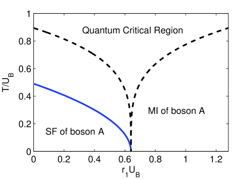
Figure 5: (Color online) The phase diagram of type A bosons at finite temperature. The parameters are set as $r_{2}U_{B}=3$, $g_{2}U_{B}^{3}=101.9$, and $g_{3}U_{B}^{3}=26.5$. $T_{c}$ is the critical line of the first-order phase transition of boson A. $T_{X}$ is the crossover line.

V Experimental proposals

The study of quantum criticality in cold-atom systems is based on in situ density measurements Zhou ; Hazzard ; Zhang ; Zhang1 . General arguments show that the observables obey universal scaling relations near the QCPs . The density can be cast as $n(\mu,T)-n_{r}(\mu,T)=T^{\frac{d}{z}+1-\frac{1}{z\nu}}G(\frac{\mu-\mu_{c}}{T^{1/z\nu}})$, where $\mu_{c}$ is the critical value of the chemical potential, $n_{r}$ is the regular part of the density and $G(x)$ is a universal function describing the singular part of the density. Following the scheme developed by Q. Zhou and T.-L. Ho Zhou we can plot the “scaled density” $A(\mu,T)\equiv T^{-\frac{d}{z}-1+\frac{1}{z\nu}}(n(\mu,T)-n_{r})$ versus $(\mu-\mu_{c})/T^{\frac{1}{\nu z}}$. The scaled density curves for all temperatures will collapse into a single curve. Here it’s important to notice that our calculation of $\nu=\frac{1}{4}$ is with respect to the argument $\delta=r_{1}-r_{1c}$. However, in the realistic cold-atom experiments we use $\mu_{1}-\mu_{1c}$ to measure the distance to the QCP. Hence, a critical exponent $\tilde{\nu}$ with respect to the argument $\mu_{1}-\mu_{1c}$ should be obtained. As we approach the tip of the insulator lob by varying the chemical potential we have Fisher $\delta=r_{1}-r_{1c}\sim(\mu_{1}-\mu_{1c})^{2}$ . A straightforward calculation yields $\tilde{\nu}=2\nu=\frac{1}{2}$. Then the scaled density will be in form of $A(\mu,T)=T^{-2}(n(\mu,T)-n_{r})$ near the first-order QCP, where we have $z=1$, $d=3$ and $\tilde{\nu}=\frac{1}{2}$. In order to distinguish this case from the second-order phase transition we also calculate the scaled density near the second-order QCP, which belongs to the three-dimensional XY universality class with critical exponents $z=1$ and $\tilde{\nu}=1$ Fisher . Then the scaled density is $A(\mu,T)=T^{-3}(n(\mu,T)-n_{r})$. By testing which form the measured scaled density obeys we can determine whether the phase transition is in first or second order.

VI Conclusions

In summary, we have investigated the quantum fluctuation effects in two-species bosons in a three-dimensional optical lattice. We find that nature of the superfluid-Mott insulator phase transition of one type of bosons can be changed from second-order to first-order by the quantum fluctuations of the other type of bosons. The scaling behavior of this first-order phase transition was studied and the critical exponents were calculated. Finally, we discussed the observation of this phenomenon in a realistic cold-atom experiment.

VII Acknowledgements

It’s a pleasure to thank Hui Zhai, Tin-Lun Ho, Xiao-Lu Yu and Zhenhua Yu for useful discussions. This work is supported by the NKBRSFC under grants Nos. 2012CB821400 and NSFC under grants Nos. 1190024.

References

- (1) Q. Zhou and T.-L. Ho, Phys. Rev. Lett. 105, 245702 (2010).
- (2) K. R. A. Hazzard and E. J. Mueller, Phys. Rev. A 84, 013604 (2011).
- (3) X. Zhang, C.-L. Hung, S.-K. Tung, N. Gemelke, and C. Chin, New J. Phys. 13, 045011 (2011).
- (4) T. Donner, S. Ritter, T. Bourdel, A. Öttl, M. Köhl, and T. Esslinger, Science 315, 1556 (2007).
- (5) X. Zhang, C.-L. Hung, S.-K. Tung, and C. Chin, Science 335, 1070 (2012).
- (6) S. Coleman and E. Weinberg, Phys. Rev. D 7, 1888 (1973).
- (7) B. I. Halperin, T. C. Lubensky, and S. -K. Ma, Phys. Rev. Lett. 32, 292 (1974).
- (8) D. J. Amit, Field theory, the renormalization group, and critical phenomena, Part II, chapter 4, 2ed, World Scientific, 1984.
- (9) C. Domb, and M. S. Green, Phase transition and critical phenomena, Vol. 6, chapter 6, Academic Press Inc. (London) LTD, 1976.
- (10) M. A. Continentino and A. S. Ferreira, Physica A 339, 461 (2004).
- (11) A. S. Ferreira, M. A. Continentino, and E. C. Marino, Phys. Rev. B 70, 174507 (2004).
- (12) K. Yang, Phys. Rev. B 77, 085115 (2008).
- (13) Y. Qi and C. Xu, Phys. Rev. B 80, 094402 (2009).
- (14) A. J. Millis, Phys. Rev. B 81, 035117 (2010).
- (15) Jian-Huang She, Jan Zaanen, Alan R. Bishop, and Alexander V. Balatsky, Phys. Rev. B 82, 165128 (2010).
- (16) S. Diehl, M. Baranov, A. J. Daley, and P. Zoller, Phys. Rev. Lett. 104, 165301 (2010).
- (17) Lars Bonnes and Stefan Wessel, Phys. Rev. Lett. 106, 185302 (2011).
- (18) J. Catani, L. DeSarlo, G. Barontini, F. Minardi, and M. Inguscio, Phys. Rev. A 77, 011603(R) (2008).
- (19) S. Trotzky et al., Science 319, 295 (2008).
- (20) G. Thalhammer, G. Barontini, L. De Sarlo, J. Catani, F. Minardi, and M. Inguscio, Phys. Rev. Lett. 100, 210402 (2008).
- (21) B. Gadway, D. Pertot, R. Reimann, and D. Schneble, Phys. Rev. Lett. 105, 045303 (2010).
- (22) J. R. Han, T. Zhang, Y. Z. Wang, and W.M. Liu, Phys. Lett. A 332, 131 (2004).
- (23) P. Buonsante, S. M. Giampaolo, F. Illuminati, V. Penna, and A. Vezzani, Phys. Rev. Lett. 100, 240402 (2008).
- (24) G. H. Chen and Y. S. Wu, Phys. Rev. A 67, 013606 (2003).
- (25) A. Isacsson, M. C. Cha, K. Sengupta, and S. M. Girvin, Phys. Rev. B 72, 184507 (2005).
- (26) Y. Li, M. R. Bakhtiari, L. He, and W. Hofstetter, Phys. Rev. A 85, 023624 (2012).
- (27) E. Altman, W. Hofstetter, E. Demler, and M. D. Lukin, N. J. Phys. 5, 113 (2003).
- (28) A. B. Kuklov and B. V. Svistunov, Phys. Rev. Lett. 90, 100401 (2003).
- (29) A. Kuklov, N. Prokof’ev, and B. Svistunov, Phys. Rev. Lett. 92, 050402 (2004).
- (30) M. Greiner, O. Mandel, T. Esslinger, T. W. Hänsch, and I. Bloch, Nature 415, 39 (2002).
- (31) T. Stöferle, H. Moritz, C. Schori, M. Köhl, and T. Esslinger, Phys. Rev. Lett. 92, 130403 (2004).
- (32) I. B. Spielman, W. D. Phillips, and J. V. Porto, Phys. Rev. Lett. 98, 080404 (2007).
- (33) M. P. A. Fisher, P. B. Weichman, G. Grinstein, and D. S. Fisher, Phys. Rev. B 40, 546 (1989).
- (34) D. Jaksch, C. Bruder, J.I. Cirac, C. W. Gardiner, and P. Zoller, Phys. Rev. Lett. 81, 3108 (1998).
- (35) S. Sachdev, Quantum Phase Transition, Cambridge University Press, 2011.
- (36) B. Nienhuis and N. Nauenberg, Phys. Rev. Lett. 35, 477 (1975).
- (37) M. E. Fisher and A. N. Berker, Phys. Rev. B 26, 2507 (1982).