Reversal mechanism of an individual Ni nanotube simultaneously studied by torque and SQUID magnetometry

Abstract

Using an optimally coupled nanometer-scale SQUID, we measure the magnetic flux originating from an individual ferromagnetic Ni nanotube attached to a Si cantilever. At the same time, we detect the nanotube’s volume magnetization using torque magnetometry. We observe both the predicted reversible and irreversible reversal processes. A detailed comparison with micromagnetic simulations suggests that vortex-like states are formed in different segments of the individual nanotube. Such stray-field free states are interesting for memory applications and non-invasive sensing.

Recent experimental and theoretical work has demonstrated that nanometer-scale magnets, as a result of their low-dimensionality, display magnetic configurations not present in their macroscopic counterparts Wang:2002 ; Streubel:2012 ; StreubelAPL:2012 . Such work is driven by both fundamental questions about nanometer-scale magnetism and the potential for applying nanomagnets as elements in high-density memories Parkin:2008 , in high-resolution imaging Khizroev:2002 ; Poggio:2010 ; Campanella:2011 , or as magnetic sensors Maqableh:2012 . Compared to nanowires, ferromagnetic nanotubes are particularly interesting for magnetization reversal as they avoid the Bloch point structure Hertel:2004 . Different reversal processes via curling, vortex wall formation, and propagation have been predicted LanderosAPL:2007 ; Escrig:2008 ; Landeros:2009 ; Landeros:2010 . Due to their inherently small magnetic moment, experimental investigations have often been conducted on large ensembles. The results, however, are difficult to interpret due to stray-field interactions and the distribution in size and orientation of the individual nanotubes BachmannJACS:2007 ; DaubJAP:2007 ; EscrigAPL:2008 ; Escrig:2008 ; BachmannJAP:2009 ; Albrecht:2011 . In a pioneering work, Wernsdorfer et al. Wernsdorfer:1996 investigated the magnetic reversal of an individual Ni nanowire at 4 K using a miniaturized SQUID. Detecting the stray magnetic flux $\Phi$ from one end of the nanowire as a function of magnetic field $\mathbf{H}$, $\Phi$ was assumed to be approximately proportional to the projection of the total magnetization $\mathbf{M}$ along the nanowire axis. At the time, $M(H)$ of the individual nanowire was not accessible and micromagnetic simulations were conducted only a decade later Hertel:2004 . Here we present a technique to simultaneously measure $\Phi(H)$ and $M(H)$ of a single low-dimensional magnet. Using a scanning nanoSQUID and a cantilever-based torque magnetometer (Fig. 1) Nagel:2013 , we investigate a Ni nanotube producing $\Phi(H)$ with a nearly square hysteresis, similar to the Ni nanowire of Ref. Wernsdorfer:1996 . $M(H)$, however, displays a more complex behavior composed of reversible and irreversible contributions, which we interpret in detail with micromagnetic simulations. In contrast to theoretical predictions, the experiment suggests that magnetization reversal is not initiated from both ends. If nanomagnets are to be optimized for storage or sensing applications, such detailed investigations of nanoscale properties are essential.

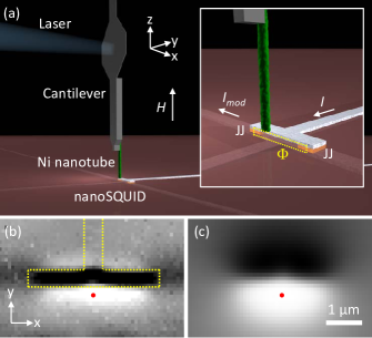
Figure 1: (Color) (a) Sketch of the apparatus (inset: zoomed-in view; dashed line indicates SQUID loop). Gray-scale maps of (b) $\Delta f(x,y)$ and (c) $\Phi(x,y)$ taken simultaneously at a distance $z=280$ nm with $H=0$. $\Delta f$ ($\Phi$) ranges from -$170$ to $430$ Hz ($-0.08\leavevmode\nobreak\ \Phi_{0}$ to $0.08\leavevmode\nobreak\ \Phi_{0}$). Dashed lines indicate the T-shaped SQUID arm and dots the operating position.

We use a direct current nanoSQUID formed by a loop containing two superconductor-normal-superconductor Josephson junctions (JJs) NagelAPL:2011 ; Wolbing:2013 ; SupMat (Fig. 1 (a)). Two T-shaped superconducting Nb arms are sputtered on top of each other separated by an insulating layer of SiO₂. The Nb arms are connected via two planar 225-nm-thick Nb/HfTi/Nb JJs each with an area of $200\times 200$ nm². These JJs and the $1.8$-$\mu$m-long Nb leads form a SQUID loop in the $xz$-plane (shown in yellow in Fig. 1 (a)), through which we measure $\Phi$. Atomic layer deposition of Ni is used to prepare the nanotube around a GaAs nanowire template grown by molecular beam epitaxy (MBE) Ruffer:2012 ; Weber:2012 . The GaAs core supports the structure, making it mechanically robust. The polycrystalline nanotube, which does not exhibit magneto-crystalline anisotropy, has a $140\pm 20$-nm outer diameter, a $70\pm 10$-nm inner diameter, and a $6.0\pm 0.5$-$\mu$m length. The error in the diameters results from the roughness of the Ni film SupMat . The Ni nanotube is affixed to the end of an ultrasoft Si cantilever Weber:2012 , such that it protrudes from the tip by $4\,\mathrm{\mu m}$. The cantilever is 120-$\mu$m-long, 4-$\mu$m-wide and 0.1-$\mu$m-thick. It hangs above the nanoSQUID in the pendulum geometry, inside a vacuum chamber (pressure $<10^{-6}$ mbar) at the bottom of a cryostat. A 3D piezo-electric positioning stage moves the nanoSQUID relative to the Ni nanotube and an optical fiber interferometer is used to detect deflections of the cantilever along $\hat{y}$ Rugar:1989 . Fast and accurate measurement of the cantilever’s fundamental resonance frequency $f_{c}$ is realized by self-oscillation at a fixed amplitude. An external field $\mu_{0}\mathbf{H}$ of up to $2.8$ T can be applied along the cantilever axis $\hat{z}$ using a superconducting magnet. At $4.3\,\mathrm{K}$ and $\mu_{0}H=0$, the cantilever, loaded with the Ni nanotube and far from any surfaces, has an intrinsic resonance frequency $f_{c}=f_{0}=3413\,\mathrm{Hz}$, a quality factor $Q=Q_{0}=3.4\times 10^{4}$, and spring constant of $k_{0}=90\pm 10\,\mathrm{\mu N/m}$. The magnetic flux due the Ni nanotube $\Phi_{\text{NN}}(H)$ is evaluated from $\Phi_{\text{NN}}(H)=\Phi(H)-\Phi_{\text{ref}}(H)$, where the flux $\Phi(H)$ is measured with the nanotube close to the nanoSQUID, while $\Phi_{\text{ref}}(H)$ is measured with the nanotube several $\mu$m away such that the stray flux is negligible. Therefore $\Phi_{\text{ref}}(H)\propto H$, due to the small fraction of $\mathbf{H}$ that couples through the nanoSQUID given its imperfect alignment with $\hat{z}$. Once calibrated, we also use $\Phi_{\text{ref}}(H)$ to measure the $\mu_{0}H$ axis of our plots, removing effects due to hysteresis in the superconducting magnet. Such a field calibration was not possible for the integrated SQUID of Ref. Wernsdorfer:1996 . We also perform dynamic-mode cantilever magnetometry Stipe:2001.2 , which is sensitive to the dynamic component of the magnetic torque acting between $\mathbf{H}$ and the magnetization $\mathbf{M}$ of the Ni nanotube. In order to extract $M(H)$, we measure the field-dependent frequency shift $\Delta f(H)=f_{c}(H)-f_{0}$. Micromagnetic simulations are performed with NMAG NMAG which provides finite-element modeling by adapting a mesh to the curved inner and outer surfaces of the nanotube. We simulate 30-nm thick nanotubes of different lengths $l$ and the same 70-nm inner diameter. We assume magnetically isotropic Ni consistent with earlier studies Ruffer:2012 , a saturation magnetization $M_{\text{S}}=406$ kA/m Kittel:2005 , and exchange coupling constant of $7\times 10^{12}$ J/m Knittel:2011 .

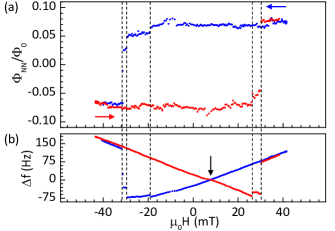
Figure 2: (Color) Simultaneously measured hysteresis loops of (a) $\Phi_{\text{NN}}(H)$ and (b) $\Delta f(H)$ at $z=450$ nm. Red (blue) points represent data taken while sweeping $H$ in the positive (negative) direction. Dashed lines indicate discontinuities (magnetic switching fields $H_{\rm sw,e}$) appearing in both $\Phi_{\text{NN}}(H)$ and $\Delta f(H)$.

We first scan the nanoSQUID under the cantilever with attached Ni nanotube, to map the coupling between them. To ensure that the scan is done with the nanotube in a well-defined magnetic state, we first saturate it along its easy axis ($\hat{z}$). Scans are then made at $H=0$ in the $xy$-plane at a fixed height $z$, i.e. for a fixed distance between the top of the SQUID device and the bottom end of the Ni nanotube. $\Delta f(x,y)=f_{c}(x,y)-f_{0}$ and $\Phi(x,y)$ are measured simultaneously, as shown in Fig. 1 (b) and (c) respectively. $\Delta f(x,y)$ is proportional to the force gradient $\partial F_{y}/\partial y$ acting on the cantilever and is sensitive to both the topography of the sample and to the magnetic field profile in its vicinity. Raised features such as the T-shaped top-electrode of the nanoSQUID are visible. $\Phi(x,y)$ shows a bipolar flux response. The change in sign of $\Phi(x,y)$ occurs as the Ni nanotube crosses the $xz$-plane (defined by the SQUID loop) above the nanoSQUID, matching the expected response. Such images allow us to identify the nanoSQUID and to position the Ni nanotube at a maximum of $|\Phi(x,y)|$. Given a constant $z$, the nanotube stray flux optimally couples through the nanoSQUID loop at such positions, resulting in the maximum signal-to-noise ratio for flux measurements.

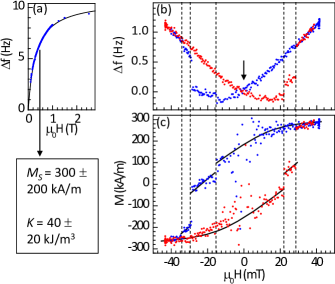
Figure 3: (Color) (a) Cantilever magnetometry (points) and fit (solid line) in large magnetic fields. (b) Cantilever magnetometry at small fields. (c) Volume magnetization $M$ extracted from (b) according to (1). Solid lines guide the eye. Red (blue) points represent data taken while sweeping $H$ in the positive (negative) direction. Dashed lines highlight switching fields $H_{\rm sw,e}$. The error in $M$ scales with $1/|H|$, explaining the scatter near $H=0$.

At one such position, indicated by the dot in Fig. 1, we record $\Phi(H)$ by sweeping $\mu_{0}H$ from 41 mT to -41 mT and vice versa. A representative hysteresis curve $\Phi_{\text{NN}}(H)=\Phi(H)-\Phi_{\text{ref}}(H)$ is shown in Fig. 2 (a) where $\Phi(H)$ is measured at $z=450\leavevmode\nobreak\$nm. $\mu_{0}|H|$ is incremented in steps of $0.2\,\mathrm{mT}$ with a wait time of $1\,\mathrm{s}$ before each acquisition. The hysteresis has an almost square shape with a maximum flux $\Phi_{\text{NN}}=75\,\mathrm{m\Phi_{0}}$ coupled into the nanoSQUID. The loop appears similar to stray-field hysteresis loops obtained from a bistable Ni nanomagnet Meier:2000 and the Ni nanowire of Ref. Wernsdorfer:1996 , where $H$ was collinear with the long axis. Such a shape may suggest that at $H=0$ the remanent magnetization $M_{\text{R}}\approx M_{\text{S}}$. Increasing $H$ from zero (see red branch in Fig. 2 (a)), we first observe a nearly constant flux, then a variation by about 30 % along with tiny jumps in a small field regime, and finally a large jump occurring near 30 mT. Similar to Ref. Wernsdorfer:1996 , our SQUID data suggest that almost all magnetic moments are reversed at once near 30 mT via a large irreversible jump, i.e. via domain nucleation and propagation.

We now turn to cantilever magnetometry, which is sensitive to $M(H)$. $\Delta f$ is first measured simultaneously with $\Phi(H)$ at $z=450$ nm, as shown in Fig. 2 (b). The torque measured via $\Delta f$ is found to exhibit tiny jumps and large abrupt changes at exactly the same switching fields $H_{\rm sw,e}$ as $\Phi_{\text{NN}}(H)$. We note that switching fields vary from sweep to sweep SupMat as was observed in the Ni nanowire of Ref. Wernsdorfer:1996 ; such behavior is expected if nucleation is involved, given its stochastic nature. Importantly, there is always a one-to-one correspondence between switching fields observed in $\Delta f$ and flux $\Phi_{\text{NN}}$ as highlighted by the dashed lines in Fig. 2. This correlation confirms that the changes in $\Delta f$ and $\Phi_{\text{NN}}$ have a single origin: the reversal of magnetic moments within the Ni nanotube.

In order to analyze $\Delta f(H)$ in terms of $M(H)$ it is important to retract the Ni nanotube from the nanoSQUID by several $\mu$m. We therefore avoid magnetic interactions with both the diamagnetic superconducting leads and the modulation current of the nanoSQUID. These interactions lead to an enhanced $\Delta f$ and a branch crossing (indicated by an arrow in Fig. 2 (b)) occurring at finite $H$ rather than at $H=0$ as was reported in Ref. Ruffer:2012 . After retracting the nanotube from the nanoSQUID, we measure $\Delta f(H)=f_{c}(H)-f_{0}$ as shown in Fig. 3. We start the acquisition at a large positive field ($\mu_{0}H=2.8\leavevmode\nobreak\ {\rm T}$), where the nanotube is magnetized to saturation and then reduce $H$ to zero as shown in Fig. 3 (a). In large fields, the nanotube behaves as a single-domain magnetic particle, i.e. it is magnetized uniformly and $M$ rotates in unison as the cantilever oscillates in the magnetic field. Based on this assumption, we fit the results with an analytical model for $\Delta f(H)$ Weber:2012 . The volume of the Ni nanotube $V_{\text{Ni}}$, $\omega_{0}$, and $k_{0}$ are set to their measured values, while the saturation magnetization $M_{\text{S}}=300\pm 200$ kA/m and the anisotropy parameter $K=40\pm 20$ kJ/m³ are extracted as fit parameters. The error in these parameters is dominated by the error associated with the measurement of the nanotube’s exact geometry and therefore of $V_{\text{Ni}}$ SupMat . $M_{\text{S}}$ is consistent with the findings of Ref. Weber:2012 on similar nanotubes and with $406$ kA/m, known as the saturation magnetization for bulk crystalline Ni at low temperature Kittel:2005 .

Figure 3 (b) shows $\Delta f(H)$ taken in the low-field regime. In an opposing field, we observe discrete steps in $\Delta f(H)$ indicating abrupt changes in the volume magnetization $M$. As expected the branch crossing (arrow) occurs at $H=0$ and the overall behavior is consistent with measurements of similar nanotubes Weber:2012 . To analyze the low field data, we adapt the analytical model to extract the dependence of the volume magnetization $M$ on $H$, i.e. the field dependence of magnetization averaged over the entire volume of the nanotube. Solving the equations of Ref. Weber:2012 describing the frequency shift for $M$, we find:

$$M=\frac{2k_{0}l_{e}^{2}K\Delta f}{H\left(KV_{\text{Ni}}f_{0}-k_{0}l_{e}^{2}\Delta f\right)},$$ (1)

where $l_{e}=85$ $\mu$m is the effective cantilever length for the fundamental mode. $M(H)$ extracted from Fig. 3 (b) is plotted in Fig. 3 (c). In both field sweep directions, the magnetization is seen to first undergo a gradual decrease as $|H|$ decreases. Starting from $\sim 300$ kA/m at +40 mT, $M$ reduces to $\sim 200$ kA/m at 0 mT. We find $M_{\text{R}}\approx 0.65\leavevmode\nobreak\ M_{\text{S}}$, in contrast with the SQUID data suggesting $M_{\text{R}}\approx M_{\text{S}}$. However, this gradual change of $M$ at small $|H|$ in the initial stage of the reversal is consistent with the gradually changing anisotropic magnetoresistance observed in a similar nanotube of larger diameter in nearly the same field regime Ruffer:2012 . At -15 mT, just before the first of three discontinuous jumps, $M$ is only $\sim 100\leavevmode\nobreak\$kA/m. Note that jumps are seen after the magnetization has decreased to a value of about $0.3\leavevmode\nobreak\ M_{\text{S}}$. Two further jumps occur at $\mu_{0}H_{\rm sw,e}=-28$ and -33 mT. For $\mu_{0}H<-40$ mT, the nanotube magnetization is completely reversed. We observe a somewhat asymmetric behavior at positive and negative fields. This asymmetry may be due to an anti-ferromagnetic NiO surface layer providing exchange interaction with the Ni nanotube Zhang:2000 ; Gierlings:2002 . Irreversible jumps in $M$ are observed for $15\leavevmode\nobreak\$mT $<\mu_{0}|H_{\rm sw,e}|<35\leavevmode\nobreak\$mT in Fig. 3, in perfect agreement with the range over which jumps occur in $\Phi_{\rm NN}$ with the nanotube close to the nanoSQUID in Fig. 2.

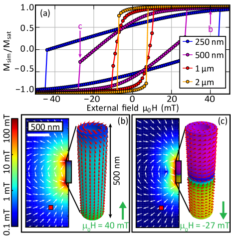
Figure 4: (Color) (a) Simulated hysteresis loops $M(H)$ for nanotubes of four different $l$. $H_{\rm sw}$ increases with decreasing $l$. Magnetic configurations (right) and stray-field distribution (left) for $l=500\leavevmode\nobreak\$nm at (b) $40\leavevmode\nobreak\$mT and (c) $-27\leavevmode\nobreak\$mT as indicated by the labels in (a). Cones (arrows) indicate the local direction of the magnetic moments (stray field). The stray fields $H_{\rm str}$ are color coded as depicted. The red squares indicate the position of the center of the nanoSQUID loop.

The observed magnetization steps suggest the presence of 2 to 4 intermediate magnetic states or 2 to 4 segments in the nanotube that switch at different $H$. Calculations for ideal nanotubes Landeros:2009 suggest that the intermediate states should be multi-domain, consisting of uniform axially saturated domains separated by azimuthal or vortex-like domain walls. The preferred sites for domain nucleation are expected to be the two ends of the nanotube Hertel:2004 ; Landeros:2009 . As the field is reduced after saturation, magnetic moments should gradually curl or tilt away from the field direction. The torque magnetometry measurements, which show both gradual and abrupt changes in $M(H)$, are consistent with such gradual tilting; the SQUID data, showing only abrupt changes in $\Phi_{\text{NN}}(H)$, are not. In the following we present micromagnetic simulations performed on Ni nanotubes of different lengths $l$ to further analyze our data.

In Fig. 4 (a) we show simulated hysteresis loops $M(H)$ with $\mathbf{H}$ applied along the long axis of nanotubes with $l$ between 250 nm and 2 $\mu$m. For $l=2\leavevmode\nobreak\ \mu$m the $M(H)$ loop is almost square, but the switching field is $\sim 8$ mT. This value is much smaller than the regime of $H_{\rm sw,e}$ observed experimentally. Nanotubes with 250 nm$\leavevmode\nobreak\ <l<1\leavevmode\nobreak\ \mu$m are consistent with $15\leavevmode\nobreak\ {\rm mT}<\mu_{0}|H_{\rm sw,e}|<35\leavevmode\nobreak\$mT . For $l=500\leavevmode\nobreak\$nm the simulation provides a switching field $\mu_{0}H_{\rm sw}=28\leavevmode\nobreak\$mT. At the same time, $M$ is almost zero for $|H|$ just below $|H_{\rm sw}|$. Such behavior is consistent with the overall shape of the measured $M(H)$ loop in Fig. 3 (c), where the largest jumps in $M$ take place at about $\pm 30\leavevmode\nobreak\$mT. Comparing Fig. 4 (a) and Fig. 3 (c), we conclude that the superposition of a few segments with $250\leavevmode\nobreak\ {\rm nm}<l<1\leavevmode\nobreak\ \mu$m could account for the measured $M(H)$. For such segments, Fig. 4 (b) and (c) (right panels) show characteristic spin configurations (cones) well above and near $H_{\rm sw}$, respectively. We observe the gradual tilting of spins at both ends in (b) and two tubular-like vortex domains with opposite circulation direction in (c) Chen:2011 . Between the domains a Néel-type wall exists. For each $l$ and $M(H)$, we simulate the relevant stray field at the position of the nanoSQUID (red squares in the left panels of Fig. 4 (b) and (c)) providing the predicted $\Phi_{\rm NN}(H)$ SupMat . The shapes of the simulated $\Phi_{\rm NN}(H)$ are nearly proportional to and thus closely follow the shape of $M(H)$ shown in Fig. 4 (a). Thus the simulations allow us to explain the measured torque magnetometry data, although they are inconsistent with the nanoSQUID data.

The contrast between hysteresis traces obtained by the nanoSQUID and torque magnetometry shows that $\Phi(H)$ is not the projection of $\mathbf{M}$ along the nanotube axis. This finding contradicts the assumption of Ref. Wernsdorfer:1996 ; we attribute this discrepancy to the fact that while cantilever magnetometry measures the entire volume magnetization, the nanoSQUID is most sensitive to the magnetization at the bottom end of the nanotube, as shown in calculations of the coupling factor $\phi_{\mu}=\Phi/\mu$ (flux $\Phi$ coupled to nanoSQUID by a point-like particle with magnetic moment $\mu$) Nagel:2013 . Still, we find a one-to-one correspondence between switching fields $H_{\rm sw,e}$ detected by either the nanoSQUID or cantilever magnetometry. This experimentally verified consistency substantiates the reversal field analysis performed in Ref. Wernsdorfer:1996 . In Fig. 2 (a), we find no clear evidence for curling or gradual tilting at small $H$. The reversal process thus does not seem to start from the end closest to the nanoSQUID, but rather from a remote segment. This is an important difference compared to the ideal nanotubes considered thus far in the literature, in which both ends share the same fate in initiating magnetization reversal. The unintentional roughness of real nanotubes might be relevant here. In an experiment performed on a large ensemble of nanotubes, one would have not been able to judge whether a gradual decrease in $M(H)$ Albrecht:2011 originated from a very broad switching field distribution or from the gradual tilting of magnetic moments in the individual nanotubes. Our combination of nano-magnetometry techniques thus represents a powerful method for unraveling hidden aspects of nanoscale reversal processes. In order to optimize nanotubes for sensing and memory applications, such understanding is critical.

In summary, we have presented a technique for measuring magnetic hysteresis curves of nanometer-scale structures using a piezo-electrically positioned nanoSQUID and a cantilever operated as a torque magnetometer. This dual functionality provides two independent and complementary measurements: one of local stray magnetic flux and the other of volume magnetization. Using this method we gain microscopic insight into the reversal mechanism of an individual Ni nanotube, suggesting the formation of vortex-like tubular domains with Néel type walls.

A. Buchter, J. Nagel, and D. Rüffer contributed equally to this work which was funded by the Canton Aargau, the SNI, the SNF under Grant No. 200020-140478, the NCCR QSIT, the DFG via the SFB/TRR 21, and the ERC via the advanced grant SOCATHES. Research leading to these results was funded by the European Community’s Seventh Framework Programme (FP7/2007-2013) under Grant Agreement No. 228673 MAGNONICS. J. Nagel acknowledges support from the Carl-Zeiss-Stiftung.

References

- (1) Z. K. Wang, M. H. Kuok, S. C. Ng, D. J. Lockwood, M. G. Cottam, K. Nielsch, R. B. Wehrspohn, and U. Gösele, Phys. Rev. Lett. 89, 027201 (2002).
- (2) R. Streubel, J. Thurmer, D. Makarov, F. Kronast, T. Kosub, V. Kravchuk, D. D. Sheka, Y. Gaididei, R. Schäfer, and O. G. Schmidt, Nano Lett. 12, 3961 (2012).
- (3) R. Streubel, V. P. Kravchuk, D. D. Sheka, D. Makarov, F. Kronast, O. G. Schmidt, and Y. Gaididei, Appl. Phys. Lett. 101, 132419 (2012).
- (4) S. S. P. Parkin, M. Hayashi, and L. Thomas, Science 320, 190 (2008).
- (5) S. Khizroev, M. H. Kryder, and D. Litvinov, Appl. Phys. Lett. 81, 2256 (2002).
- (6) M. Poggio and C. L. Degen, Nanotechnology 21, 342001 (2010).
- (7) H. Campanella, M Jaafar, J. Llobet, J. Esteve, M. Vázquez, A. Asenjo, R. P. del Real, and J. A. Plaza, Nanotechnology 22, 505301 (2011).
- (8) M. M. Maqableh, X. Huang, S.-Y. Sung, K. S. M. Reddy, G. Norby, R. H. Victora, and B. J. H. Stadler Nano Lett., 12, 4102 (2012).
- (9) R. Hertel and J. Kirschner, J. Magn. Magn. Mater. 278, L291 (2004).
- (10) P. Landeros, O. J. Suarez, A. Cuchillo, and P. Vargas, Phys. Rev. B 79, 024404 (2009).
- (11) P. Landeros and Á. S. Núñez, J. Appl. Phys. 108, 033917 (2010).
- (12) J. Escrig, J. Bachmann, J. Jing, M. Daub, D. Altbir, and K. Nielsch, Phys. Rev. B 77, 214421 (2008).
- (13) P. Landeros, S. Allende, J. Escrig, E. Salcedo, D. Altbir, and E. E. Vogel, Appl. Phys. Lett. 90, 102501 (2007).
- (14) J. Bachmann, J. Jing, M. Knez, S. Barth, H. Shen, S. Mathur, U. Gösele, and K. Nielsch, J. Am. Chem. Soc. 129, 9554 (2007).
- (15) M. Daub, M. Knez, U. Goesele, and K. Nielsch, J. Appl. Phys. 101, 09J111 (2007).
- (16) J. Bachmann, J. Escrig, K. Pitzschel, J. M. Montero Moreno, J. Jing, D. Görlitz, D. Altbir, and K. Nielsch, J. Appl. Phys. 105, 07B521 (2009).
- (17) O. Albrecht, R. Zierold, S. Allende, J. Escrig, C. Patzig, B. Rauschenbach, K. Nielsch, and D. Görlitz, J. Appl. Phys. 109, 093910 (2011).
- (18) J. Escrig, S. Allende, D. Altbir, and M. Bahiana, Appl. Phys. Lett. 93, 023101 (2008).
- (19) W. Wernsdorfer, B. Doudin, D. Mailly, K. Hasselbach, A. Benoit, J. Meier, J.-Ph. Ansermet, and B. Barbara, Phys. Rev. Lett. 77, 1873 (1996).
- (20) J. Nagel, A. Buchter, Fei Xue, O. F. Kieler, T. Weimann, J. Kohlmann, A. B. Zorin, D. Rüffer, E. Russo-Averchi, R. Huber, P. Berberich, A. Fontcuberta i Morral, D. Grundler, R. Kleiner, D. Koelle, M. Poggio, and M. Kemmler, arXiv:1305.1195 (2013).
- (21) J. Nagel, O. F. Kieler, T. Weimann, R. Wölbing, J. Kohlmann, A. B. Zorin, R. Kleiner, D. Koelle and M. Kemmler, Appl. Phys. Lett. 99, 032506 (2011).
- (22) R. Wölbing, J. Nagel, T. Schwarz, O. Kieler, T. Weimann, J. Kohlmann, A. Zorin, M. Kemmler, R. Kleiner, and D. Koelle, Appl. Phys. Lett., in press; arXiv:1304.7584 (2013).
- (23) See supplementary material.
- (24) D. Rüffer, R. Huber, P. Berberich, E. Russo-Averchi, M. Heiss, J. Arbiol, A. Fontcuberta i Morral, and D. Grundler, Nanoscale 4, 4989 (2012).
- (25) D. P. Weber, D. Rüffer, A Buchter, F. Xue, E. Russo Averchi, R. Huber, P. Berberich, J. Arbiol, A. Fontcuberta i Morral, D. Grundler, and M. Poggio, Nano Lett., 12, 6139 (2012).
- (26) D. Rugar, H. J. Mamin, and P. Guethner, Appl. Phys. Lett. 55, 2588 (1989).
- (27) B. C. Stipe, H. J. Mamin, T. D. Stowe, T. W. Kenny, and D. Rugar, Phys. Rev. Lett. 86, 2874 (2001).
- (28) T. Fischbacher, M. Franchin, G. Bordignon, H. Fangohr, IEEE Trans. Magn. 43, 2896 (2007); http://nmag.soton.ac.uk/nmag/.
- (29) C. Kittel, Introduction to Solid-State Physics, 8th ed. (Wiley, 2005).
- (30) A. Knittel, Micromagnetic simulations of three dimensional core-shell nanostructures, Ph.D. dissertation, University of Southampton (2011).
- (31) G. Meier, D. Grundler, K.-B. Broocks, Ch. Heyn, and D. Heitmann, J. Magn. Magn. Mater. 210, 138 (2000).
- (32) P. Zhang, F. Zuo, F. K. Urban III, A Khabari, P. Griffiths, and A. Hosseini-Tehrani, J. Magn. Magn. Mater. 225, 337 (2000).
- (33) M. Gierlings, M. J. Prandolini, H. Fritzsche, M. Gruyters, and D. Riegel, Phys. Rev. B 65, 092407 (2002).
- (34) A.-P. Chen, J. M. Gonzalez, and K. Y. Guslienko, J. Appl. Phys. 109, 073923 (2011).