The quest for companions to post-common envelope binaries

We present 69 new mid-eclipse times of the young post-common envelope binary (PCEB) NN Ser, which was previously suggested to possess two circumbinary planets. We have interpreted the observed eclipse-time variations in terms of the light-travel time effect caused by two planets, exhaustively covering the multi-dimensional parameter space by fits in the two binary and ten orbital parameters. We supplemented the fits by stability calculations for all models with an acceptable $\,\chi^{2}$. An island of secularly stable 2 : 1 resonant solutions exists, which coincides with the global $\,\chi^{2}$ minimum. Our best-fit stable solution yields current orbital periods $P_{\mathrm{o}}\!=\!15.47$ yr and $P_{\mathrm{i}}\!=\!\,7.65$ yr and eccentricities $e_{\mathrm{o}}\!=\!0.14$ and $e_{\mathrm{i}}\!=\!0.22$ for the outer and inner planets, respectively. The companions qualify as giant planets, with masses of 7.0 $M_{\mathrm{Jup}}$ and 1.7 $M_{\mathrm{Jup}}$ for the case of orbits coplanar with that of the binary. The two-planet model that starts from the present system parameters has a lifetime greater than $10^{8}$ yr, which significantly exceeds the age of NN Ser of $10^{6}$ yr as a PCEB. The resonance is characterized by libration of the resonant variable $\Theta_{1}$ and circulation of $\omega_{\mathrm{i}}\!-\!\omega_{\mathrm{o}}$, the difference between the arguments of periapse of the two planets. No stable nonresonant solutions were found, and the possibility of a 5 : 2 resonance suggested previously by us is now excluded at the 99.3% confidence level.

1 Introduction

Planets orbiting post-common envelope binaries (PCEB) are a recent discovery, and only a few PCEB are known or suspected to harbor planetary systems. These planets are detected by the light-travel time (LTT) effect, which measures the variations in the observed mid-eclipse times caused by the motion of the binary about the common center of mass. The derived orbital periods significantly exceed those of planets orbiting single stars, because the LTT method preferably selects long orbital periods and the radial-velocity and transit methods short ones. Since eclipse-time variations can also be brought about by other mechanisms, it is necessary to prove the strict periodicity of the LTT signal to confirm its planetary origin. The orbital periods on the order of a decade represent a substantial challenge, however. For a system of circumbinary planets, one additionally has to demonstrate the secular stability of a particular solution.

The discovery of two planets orbiting the dG/dM binary Kepler 47 with semi-major axes less than 1 AU (Orosz et al., 2012) has convincingly demonstrated that close binaries can possess planetary systems, but also raised questions about their orbital co-evolution. The evolutionary history of planets orbiting PCEB may be complex: they either formed before the common-envelope (CE) event and had to survive the loss of a substantial amount of matter from the evolving binary and the passage through the ejected shell, or they were assembled later from CE-material. Even if the planets existed before the CE, their masses may have increased in the CE by accretion, making a distinction between first and second-generation origins difficult. In both cases the CE may have significantly affected the planetary orbits, and we expect that the dynamical age of the system equals the age of the PCEB, which is the cooling age of the white dwarf. The hot white dwarf in NN Ser has an age of only $10^{6}$ yr (Parsons et al., 2010a), so the planets in NN Ser are dynamically young. Migration of planets is expected to occur in the CE, but our poor knowledge of the CE structure complicates predictions about the dynamical state of PCEB planetary systems.

Only a handful of PCEB have been suggested to contain more than one circumbinary companion. Of these, NN Ser (Beuermann et al., 2010; Horner et al., 2012) and HW Vir (Beuermann et al., 2012) have passed the test of secular stability. A final conclusion on HU Aqr (Goździewski et al., 2012; Hinse et al., 2012) is pending, and the eclipse-time variations in QS Vir are presently not understood (Parsons et al., 2010b). For a few other contenders, the data are still insufficient for theoretical modeling. In the case of NN Ser, a period ratio of the two proposed planets near either 2 : 1 or 5 : 2 was found (Beuermann et al. 2010, henceforth Paper I), with both models being stable for more than $10^{6}$ yr. Horner et al. (2012) confirm the dynamical stability of the proposed orbits, but suggest that further observations are vital in order to better constrain the system’s true architecture. In this paper, we report further eclipse-time observations of NN Ser and present the results of extensive stability calculations, which show that a two-planet system that starts from our best fit will be secularly stable and stay tightly locked in the 2 : 1 mean-motion resonance for more than $10^{8}$ yr.

2 Observations

Table 1: Mid-eclipse times of NN Ser measured with MONET/N.

Cycle	JD	Error	BJD(TDB)	$O\!-\!C_{\mathrm{ell}}$
	2450000+	(days)	2450000+	(s)
(a) January /February 2010 (Paper I).
60489	5212.9431997	0.0000069	5212.9418190	0.20
60505	5215.0243170	0.0000067	5215.0230965	$-$0.17
60528	5218.0159241	0.0000044	5218.0149383	$-$0.23
60735	5244.9402624	0.0000029	5244.9415257	0.09
60743	5245.9808144	0.0000032	5245.9821657	0.02
60751	5247.0213676	0.0000034	5247.0228067	0.02
60774	5250.0129571	0.0000034	5250.0146473	$-$0.16
(b) September 2010 to February 2013 (this work).
62316	5450.5995341	0.0000052	5450.5981913	$-$0.35
62339	5453.5916006	0.0000067	5453.5900372	$-$0.10
62347	5454.6323120	0.0000067	5454.6306732	$-$0.53
62462	5469.5925302	0.0000049	5469.5899042	0.87
62531	5478.5685430	0.0000051	5478.5654275	0.39
63403	5591.9955682	0.0000030	5591.9953015	0.20
63449	5597.9787495	0.0000031	5597.9789848	$-$0.06
63457	5599.0193095	0.0000027	5599.0196329	0.55
63472	5600.9703359	0.0000067	5600.9708248	$-$0.33
63671	5626.8541370	0.0000041	5626.8567788	0.21
63672	5626.9842067	0.0000037	5626.9868588	0.20
63679	5627.8946901	0.0000041	5627.8974134	$-$0.35
63740	5635.8289827	0.0000044	5635.8323043	$-$0.15
63741	5635.9590539	0.0000049	5635.9623850	$-$0.10
63756	5637.9101120	0.0000042	5637.9135830	$-$0.45
63833	5647.9256179	0.0000033	5647.9297557	$-$0.30
63864	5651.9578679	0.0000046	5651.9622470	0.30
63879	5653.9089538	0.0000031	5653.9134435	$-$0.19
63886	5654.8194618	0.0000037	5654.8240016	$-$0.44
63925	5659.8923285	0.0000038	5659.8971306	$-$0.14
63933	5660.9329164	0.0000053	5660.9377686	$-$0.42
64079	5679.9239504	0.0000038	5679.9294753	0.08
64086	5680.8344900	0.0000039	5680.8400351	$-$0.02
64116	5684.7368230	0.0000052	5684.7424416	0.17
64132	5686.8180703	0.0000035	5686.8237195	$-$0.22
64784	5771.6337400	0.0000040	5771.6359752	$-$0.30
64869	5782.6914476	0.0000067	5782.6927870	$-$0.40
64938	5791.6677191	0.0000043	5791.6683161	$-$0.52
64961	5794.6598199	0.0000041	5794.6601694	0.33
64976	5796.6111770	0.0000036	5796.6113657	$-$0.19

Table 1 continued

Cycle	JD	Error	BJD(TDB)	$O\!-\!C_{\mathrm{ell}}$
	2450000+	(days)	2450000+	(s)
64992	5798.6926278	0.0000045	5798.6926456	$-$0.42
65053	5806.6281610	0.0000047	5806.6275377	$-$0.18
65081	5810.2706975	0.0000040	5810.2697878	0.32
65084	5810.6609723	0.0000097	5810.6600323	0.67
65099	5812.6123145	0.0000027	5812.6112242	$-$0.23
65099	5812.6123171	0.0000048	5812.6112268	$-$0.01
65360	5846.5653892	0.0000036	5846.5621492	0.13
65460	5859.5738976	0.0000089	5859.5701607	$-$0.24
65963	5925.0031268	0.0000080	5925.0004922	0.66
65994	5929.0353491	0.0000050	5929.0329653	$-$0.38
66209	5957.0004918	0.0000035	5957.0002090	0.32
66324	5971.9584470	0.0000038	5971.9594273	0.25
66332	5972.9990053	0.0000056	5973.0000740	0.71
66362	5976.9010792	0.0000080	5976.9024783	0.65
66370	5977.9416245	0.0000044	5977.9431113	$-$0.07
66409	5983.0143233	0.0000047	5983.0162339	$-$0.42
66416	5983.9248143	0.0000036	5983.9268000	0.01
66615	6009.8088279	0.0000045	6009.8127551	0.12
66631	6011.8899714	0.0000029	6011.8940322	$-$0.36
66669	6016.8327239	0.0000032	6016.8370844	0.14
66670	6016.9627977	0.0000028	6016.9671658	0.24
66677	6017.8733096	0.0000033	6017.8777301	0.50
66685	6018.9138903	0.0000027	6018.9183694	0.33
66815	6035.8235355	0.0000061	6035.8287909	0.25
66893	6045.9694909	0.0000055	6045.9750363	$-$0.44
66900	6046.8800348	0.0000041	6046.8855994	$-$0.28
66908	6047.9206573	0.0000031	6047.9262424	$-$0.14
67284	6096.8315332	0.0000034	6096.8363914	0.13
67330	6102.8155143	0.0000035	6102.8200727	$-$0.46
67337	6103.7261262	0.0000028	6103.7306356	$-$0.32
67352	6105.6774387	0.0000036	6105.6818401	$-$0.16
67675	6147.6963688	0.0000058	6147.6977420	0.19
67698	6150.6884525	0.0000041	6150.6895788	$-$0.45
67775	6160.7054661	0.0000046	6160.7057628	0.42
67928	6180.6093127	0.0000034	6180.6080271	0.11
67936	6181.6500361	0.0000036	6181.6486726	0.46
68028	6193.6182396	0.0000047	6193.6160366	$-$0.65
69168	6341.9060724	0.0000028	6341.9074599	0.06
69575	6394.8450806	0.0000020	6394.8500987	0.04

We obtained 69 additional mid-eclipse times of the 16.8 mag binary with the MONET/North telescope at the University of Texas’ McDonald Observatory via the MONET browser-based remote-observing interface. The photometric data were taken with an Apogee ALTA E47+ 1k$\times$1k CCD camera mostly in white light with 10 s exposures separated by 3 s readout. In most cases photometry was performed relative to a comparison star 2.0 arcmin SSW of NN Ser, but in some nights absolute photometry yielded lower uncertainties. The eclipse light curves were analyzed with the white dwarf represented by a uniform disk occulted by the secondary star (see Backhaus et al., 2012). A seven-parameter fit was made to each individual eclipse profile of the relative or absolute source flux. The free parameters of the fit were the mid-eclipse time $T_{\mathrm{c}}$, the fluxes outside and inside eclipse, the FWHM of the profile, the ingress/egress time, and the two parameters $a_{1}$ and $a_{2}$ of a multiplicative function $f\!=\!1+a_{1}(t-T_{\mathrm{c}})+a_{2}(t-T_{\mathrm{c}})^{2}$, which allowed us to model photometric variations outside of the eclipse. Such variations can be caused by effects intrinsic to the source, as the illumination of the secondary star, or by observational effects, as color-dependent atmospheric extinction. The formal 1-$\sigma$ error of $T_{\mathrm{c}}$ was calculated from the measurement errors of the fluxes in the individual CCD images, employing standard error propagation. The distribution of the measured FWHM of all eclipses is Gaussian with a mean of 569.20 s and a standard deviation of 0.79 s. In columns 1–3 of Table 1 we list the cycle numbers, the observed mid-eclipse times $T_{\mathrm{c}}$ in UTC, and the 1-$\sigma$ errors of the 69 new eclipses. Re-analysis of earlier MONET/N data led to small corrections, and we also include the seven mid-eclipse times published already in Paper I. The errors of $T_{\mathrm{c}}$ vary between 0.17 and 0.83 s, depending on the quality of the individual light curves. The mean timing error is 0.38 s. All mid-eclipse times were converted from Julian days (UTC) to barycentric dynamical time (TDB) and corrected for the light travel time to the solar system barycenter, using the tool provided by Eastman et al. (2010). These corrected times are given as barycentric Julian days in TDB in column 4 of Table 1. Together with the errors in column 3, they represent the new data subjected to the LTT fit in the Section 4.1.

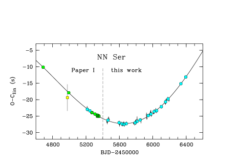
Figure 1: Residuals of the mid-eclipse times of NN Ser since 2007 relative to the linear ephemeris of Eq. 1, with the best-fitting model of Fig. 5 and Table 4 shown as solid curve. See text for further explanation.

Figure 1 shows the $O\!-\!C_{\mathrm{lin}}$ residuals relative to the linear ephemeris of the binary quoted in Eq. 1 and derived in Sect. 4.1 below. The data points to the left of the dashed line are from Paper I and those to the right from this work. The residuals of the individual MONET eclipse times are displayed as crosses with error bars. Overplotted are the weighted mean $O\!-\!C$ values for 19 groups of timings typically collected in the dark periods of individual months (cyan-blue filled circles). Plotting these mean values avoids cluttering up the graphs on the expanded ordinate scales in Figs. 5 and 6. All fits presented in this paper were made to the total set of 121 individual mid-eclipse times, 52 from Paper I and 69 from this work. The solid curve in Fig. 1 represents the best-fit two-planet LTT model derived in Sect. 4.1. The residuals $O\!-\!C_{\mathrm{ell}}$ of the individual timings relative to this fit are included in column 5 of Table 1. The new feature that allows us to derive a significantly improved orbital solution within the framework of the two-planet LTT model is the detection of the upturn in $O\!-\!C_{\mathrm{lin}}$ that commences near JD 2455650.

3 General approach

In this paper, we adopt a purely planetary explanation of the eclipse-time variations in NN Ser and represent the set of mid-eclipse times by the sum of the linear ephemeris of the binary and the LTT effect of two planets. A model that only involves a single planet was already excluded in Paper I and is not discussed again, given the very poor fit with a reduced $\,\chi^{2}_{\nu}\!=\!40.3$. Specifically, we describe the motion of the center of mass of the binary in barycentric coordinates by the superposition of two Kepler ellipses, which reflect the motion of the planets (Irwin, 1952, Eq. 1; Kopal, 1959, Eq. 8-94, Beuermann et al., 2012, Eq. 2; Paper I, Eq. 1). We justify the Keplerian model at the end of this section.

The central binary was treated as a single object with the combined mass of the binary components $M_{\mathrm{bin}}\!=\!0.646$ $M_{\odot}$, (Parsons et al., 2010a). This approach is justified, because the gravitational force exerted by the central binary on either of the planets varies only by a fraction of $10^{-7}$ or less over the binary period. Hence, the NN Ser system was treated as a triple consisting of the central object and two planets. We assumed coplanar planetary orbits viewed edge-on, which coincide practically with the orbital plane of the binary with an inclination $i_{\mathrm{bin}}\!=\!89.6^{\circ}\pm 0.2^{\circ}$ (Parsons et al., 2010a). In spite of the high inclination, transit events, which would present proof of the planetary hypothesis, are unfortunately extremely improbable. Accurate eclipse-time measurements over a sufficiently large number of orbits could, in principle, provide information on the inclinations of the gravitationally interacting orbits, but this is presently not feasible given the long periods of the planets in NN Ser. The measured orbital periods and amplitudes of the LTT effect yield minimum masses, with the true masses scaling as 1/sin $i_{\mathrm{k}}$, where $i_{\mathrm{k}}$ is the unknown inclination of planet $k$. The semi-major axes depend on the total system mass, implying a minor dependence on $i_{\mathrm{k}}$.

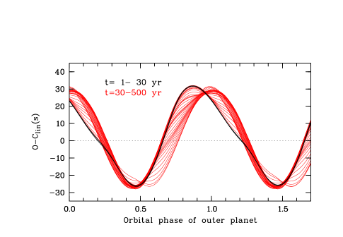
Figure 2: Temporal variation of the mid-eclipse times of NN Ser as predicted by our best-fitting dynamical two-planet model of Table 4 relative to the underlying linear ephemeris of the binary and folded over the orbital period of the outer planet. The first two orbits, covering a time interval of 30 yr (black curves), and the next 29 orbits (30–500 yr, red curves) are displayed.

Even with the new data, the least-squares fits of the LTT model permit a wide range of model parameters. As in Paper I, we required, therefore, that an acceptable model provides a good fit to the data and fulfills the side condition of secular stability. Formally, a minimum lifetime of only $10^{6}$ yr is required, the cooling age of the white dwarf and the age of NN Ser as a PCEB, but most models in the vicinity of the best fit reached more than $10^{8}$ yr, suggesting that a truly secularly stable solution exists.

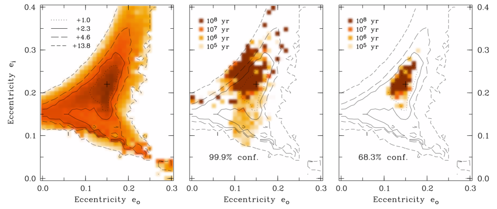
Figure 3: Results of fitting the Keplerian two-planet model to the eclipse-time data of NN Ser. Left:  $\chi^{2}$ distribution in the $e_{\mathrm{o}}$,$e_{\mathrm{i}}$ plane. The + sign indicates the minimum  $\chi^{2}$ and the contour lines refer to the increments $\Delta\,\chi^{2}$ indicated in the legend. Center: Maximum lifetime $\tau$ of models with $\chi^{2}$ at the 99.9% confidence level ($\Delta\,\chi^{2}\!=\!+13.8$ for two degrees of freedom). For ease of comparison, the  $\chi^{2}$ contours of the left panel are included. Right: Same for models with $\chi^{2}$ at the 68.3% confidence level ($\Delta\,\chi^{2}\!=\!+2.3$).

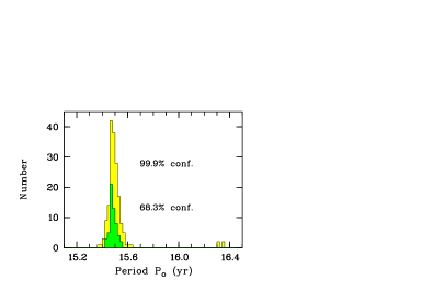
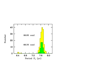
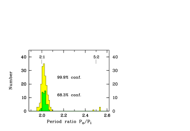
Figure 4: Histograms of the orbital periods $P_{\mathrm{o}}$ and $P_{\mathrm{i}}$ of the outer and inner planets of NN Ser and the period ratio $P_{\mathrm{o}}/P_{\mathrm{i}}$for solutions with a lifetime exceeding $10^{6}$ yr and a $\,\chi^{2}$ corresponding to the 99.9% confidence level (yellow) or the 68.3% confidence level (green) for two degrees of freedom.

We performed a large number of least-squares fits in search of the global $\,\chi^{2}$ minimum, using the Levenberg-Marquardt minimization algorithm implemented in mpfit of IDL (Marquardt, 1963; Markwardt, 2009). The time evolution of all models that achieved a $\,\chi^{2}$ below a preset limit (Sect. 4.1) was followed numerically until they became either unstable or reached a lifetime of $10^{8}$ yr. Most models that fit the data developed an instability within a few hundred years or less and fewer than 200 survived for $10^{8}$ yr, allowing us to calculate the evolution of all models with an acceptable overall CPU-time requirement. We used the hybrid symplectic integrator in the mercury6 package (Chambers, 1999), which allows one to evolve planetary systems very efficiently with high precision over long times. The model treats the central object and the planets as point masses and angular momentum and energy are conserved to a high degree of accuracy. Time steps of 0.1 yr were used, which is not adequate for the treatment of close encounters, but such incidents do not occur in the successful models (see Beuermann et al. 2012 for more details).

These dynamical model calculations provide us with information on the complex time variations of the orbital parameters, but also allow us to test the validity of the Keplerian assumption in fitting the data. Figure 2 shows the calculated variation of the mid-eclipse times for the first 500 yr of our best-fit longlived model, starting from the Keplerian fit. The LTT effect is displayed folded over the 15.47-yr orbital period of the outer planet, which contributes 87% of the signal. The first two orbits (30 yr) agree closely and are indistinguishable from the Keplerian fit, but in the long run the signal changes due to the dynamical evolution. The orbital phase interval covered in Fig. 2 is the same as in Fig 5 (top panel), where the data and the Keplerian fit are displayed. We conclude that in this special case fitting the data by a Keplerian model is justified. Data trains that extend over more orbits or involve more massive companions will require a dynamical model.

4 Results

Our least-squares fit to the 121 mid-eclipse times involves twelve free parameters, two for the linear ephemeris of the binary, the epoch $T_{\mathrm{bin}}$ and period $P_{\mathrm{bin}}$, and five orbital elements for each planet. With all parameters free, the number of degrees of freedom of the fit is therefore 109. The five parameters for planet $k$ are the orbital period $P_{\mathrm{k}}$, the eccentricity $e_{\mathrm{k}}$, the argument of periapse $\omega_{\mathrm{bin,k}}$ measured from the ascending node in the plane of the sky, the time $T_{\mathrm{k}}$ of periapse passage, and the amplitude of the eclipse time variation, $K_{\mathrm{bin,k}}=a_{\mathrm{bin,k}}$ sin $i_{\mathrm{k}}$/c, with $a_{\mathrm{bin,k}}$ the semi-major axis of the orbit of the center of mass of the binary about the common center of mass of the system, $i_{\mathrm{k}}$ the inclination of the planet’s orbit against the plane of the sky, and c the speed of light. The arguments of periapse of the center of mass of the binary (with the index ‘bin’) and that of the planet differ by $\pi$. For clarity, we use the indices k=i or k=o for the inner and outer planets, respectively .

We fitted a total of 101,618 models to the data, adopting three lines of approach. Run 1 with 81,552 models is a grid search in the $e_{\mathrm{o}}$,$e_{\mathrm{i}}$ plane. In Run 2 with 10,598 models, we started again from the $e_{\mathrm{o}}$,$e_{\mathrm{i}}$ grid values, but subsequently optimized the eccentricities along with the other parameters. Run 3 with 9,468 models was performed to study the properties of selected solutions, in particular, models in the vicinity of the best fit. It also includes models with a circular outer orbit, as advocated in Paper I, but dismissed now and not discussed further in this paper.

4.1 Grid search in the $e_{\mathrm{o}},e_{\mathrm{i}}-$plane

The grid search in the $e_{\mathrm{o}}$,$e_{\mathrm{i}}$ plane covers eccentricities from zero to 0.40 in steps of 0.01, with an extension to $e_{\mathrm{o}}\!=\!0.70$ in steps of 0.05. The ten other parameters were optimized, starting from values chosen randomly within conservative limits. Figure 3 (left panel) shows the resulting $\,\chi^{2}$ distribution for $e_{\mathrm{o}}\!<\!0.3$. For each grid point, the figure displays the best $\,\chi^{2}$ value of typically 50 model fits. The minimum is attained at $e_{\mathrm{o}},e_{\mathrm{i}}\!=\!0.15,0.22$ with $\chi^{2}_{\mathrm{min}}\!=\!95.4$. In the extension of the grid to $e_{\mathrm{o}}\!=\!0.70$, no model fit with $\chi^{2}\!<\!150$ was found. The contour lines refer to increments $\Delta\chi^{2}$ of +1.0, +2.3, +4.6, and +13.8, corresponding to confidence levels of 40%, 68.3%, 90.0%, and 99.9% for two degrees of freedom. Color coding displays the lowest $\,\chi^{2}$ as dark red, fading into white at the 99.9% level. The 68.3% contour encloses a substantial fraction of the $e_{\mathrm{o}}$,$e_{\mathrm{i}}$ plane, indicating that the data permit fits with a wide range of eccentricities and appropriate adjustment of the remaining parameters. Notably, those describing the inner planet are not well defined by the data alone, and the independent stability information is required for further selection.

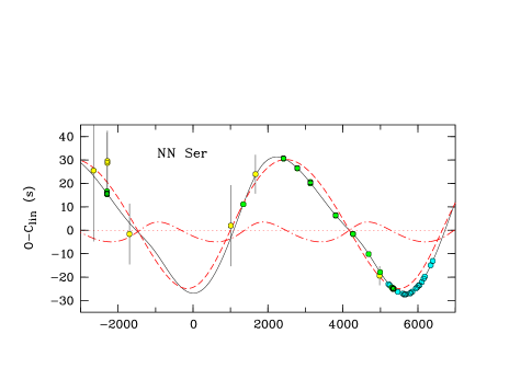
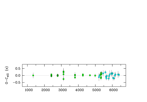
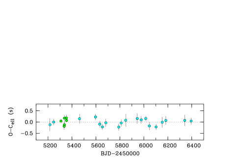
Figure 5: Best fit of the Keplerian two-planet model to the eclipse-time variations of NN Ser. The lower panels display the residuals from the fit for two different time intervals. Data points with errors larger than 1 s are omitted.

We calculated the temporal evolution of all models with $\,\chi^{2}\!<\!110$ (99.93% confidence level), starting from the fit parameters and requiring that the lifetime $\tau$ exceeds the age of NN Ser of $10^{6}$ yr. We found that an island of secularly stable models is located close to the minimum $\,\chi^{2}$, establishing an internal consistency between the fits to the data and the results of the stability calculations. The requirement of $\tau\!>\!10^{6}$ yr imposes severe constraints on the orbital parameters of the successful models and, not surprisingly, the minimum $\,\chi^{2}$ of the stable models is slightly inferior to that of the unconstrained fits. The best stable model has $\chi^{2}_{\mathrm{min}}\!=\!95.6$, eccentricities $e_{\mathrm{o}},e_{\mathrm{i}}\!=\!0.14,0.21$, and a lifetime $\tau\!=\!5\times 10^{6}$ yr. The center panel of Fig. 3 shows the lifetime distribution in the $e_{\mathrm{o}}$,$e_{\mathrm{i}}$-plane, with the peak lifetime in each bin displayed. The detailed structure of the lifetime distribution is complex. In particular, the appearance of secularly stable solutions outside the main island of stability is reminiscent of a skerry landscape. These solutions fit the data less well and disappear if the $\,\chi^{2}$ limit is reduced or, to stay in the picture, the sea level is raised. This is shown in the righthand panel of Fig. 3, where only solutions with $\tau\!>\!10^{6}$ yr and $\,\chi^{2}\!<\!97.9$ are retained (68.3% confidence). The efficiency of the lifetime selection is demonstrated by the reduced size of the island of stability, which covers only a fraction of the $\,\chi^{2}$-space delineated by the 1-$\sigma$ contour level in the lefthand panel (solid curve). Its size decreases a bit further if the eccentricities are also optimized as done in Run 2.

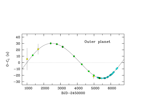
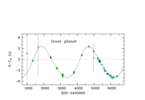
Figure 6: Residuals for the outer planet after subtracting the contribution of the inner planet (top) and vice versa (bottom). The abscissa divisions are the same for the two panels. The residuals from the fit are identical to those of Fig. 5.

We combined the results of Runs 1 and 2 to investigate the spread of the fit parameters for the solutions that pass the lifetime criterion, irrespective of their position in the $e_{\mathrm{o}}$.$e_{\mathrm{i}}$ plane. Figure 4 shows the distributions of the orbital periods $P_{\mathrm{o}}$ and $P_{\mathrm{i}}$ and the period ratio $P_{\mathrm{o}}/P_{\mathrm{i}}$ for model fits with $\,\chi^{2}\!<\!109.4$ and $\,\chi^{2}\!<\!97.9$, corresponding to the selections in the center and righthand panels of Fig. 3, respectively. For the more lenient $\,\chi^{2}$ limit, 169 of 173 solutions yield nearly identical periods and a period ratio of 2.022 with a standard deviation $\sigma\!=\!0.025$. The remaining four solutions interestingly have a period ratio of 2.512 with $\sigma\!=\!0.026$. The requirement of long-term stability implies that resonant solutions are selected, preferably the 2 : 1 case, but also 5 : 2 for a few fits. Other period ratios do not occur and no nonresonant secularly stable model was found in the entire parameter space. The stability island, together with all long-lived outliers (dark red) in the center panel of Fig. 3, represents the 2 : 1 case, while the four 5 : 2 solutions lie in the light red region around $e_{\mathrm{o}},e_{\mathrm{o}}\!=\!0.12,0.14$ on a $\,\chi^{2}$ ridge. The most longlived of the four has $\tau\!=\!6.7\times 10^{6}$ yr with $\,\chi^{2}\!=\!106.0$ and the best-fitting $\tau\!=\!1.1\times 10^{6}$ yr with $\chi^{2}\!=\!105.6$, clearly inferior to the island solutions. We exclude the 5 : 2 resonant solution at the 99.3% confidence level. Truly long-term stable solutions that provide good fits to the data exist only in the 2 : 1 mean-motion resonance explored in more detail in the next section.

Table 2: Observed and derived parameters of the Keplerian two-planet LTT model for NN Ser.

Parameter	Island solutions	Best fit
(a) Observed parameters:
Period $P_{\mathrm{o}}$  (yr)	$15.482\pm 0.027$	15.473
Period $P_{\mathrm{i}}$  (yr)	$7.647\pm 0.058$	7.653
Period ratio	$2.025\pm 0.018$	2.022
Eccentricity $e_{\mathrm{o}}$	$0.142\pm 0.011$	0.144
Eccentricity $e_{\mathrm{i}}$	$0.223\pm 0.019$	0.222
LTT amplitude $K_{\mathrm{bin,o}}$ (s)	$27.65\pm 0.12$	27.68
LTT amplitude $K_{\mathrm{bin,i}}$  (s)	$4.32\pm 0.22$	4.28
Argument of periapse $\omega_{\mathrm{bin,o}}$  (∘)	$317.0\pm\,6.4$	318.4
Argument of periapse $\omega_{\mathrm{bin,i}}$  (∘)	$48.0\pm\,2.6$	47.5
$\chi^{2}$ for 109 degrees of freedom	$<\!97.9$	95.56
Periapse passage $T_{\mathrm{o}}$  (BJD)	$2\,456\,145\pm 80$
Periapse passage $T_{\mathrm{i}}$  (BJD)	$2\,454\,406\pm 20$
(b) Derived parameters:
Outer planet, semi-major axis $a_{\mathrm{o}}$ (AU)	$5.389\pm 0.045$	5.387
Inner planet, semi-major axis $a_{\mathrm{i}}$ (AU)	$3.358\pm 0.033$	3.360
Outer planet, mass $M_{\mathrm{o}}$ sin $i_{\mathrm{o}}$  ($M_{\mathrm{Jup}}$)	$6.96\pm 0.12$	6.97
Inner planet, mass $M_{\mathrm{i}}$ sin $i_{\mathrm{i}}$  ($M_{\mathrm{Jup}}$)	$1.74\pm 0.09$	1.73

Reducing the $\,\chi^{2}$ limit to the 1-$\sigma$ level of 97.9 leaves us with 56 solutions with $\tau\!>\!10^{6}$ yr, 44 from Run-1 and 12 from Run-2 (Fig. 3, righthand panel, and Fig. 4, green histograms). In the multi-dimensional parameter space, these solutions lie close together and all parameters have narrow quasi-Gaussian distributions with well-defined mean values, as shown for the periods and the period ratio in Fig. 4. Some of the parameters are strongly correlated. We quote in Table 4 the mean values and the standard deviations of the respective parameters with all other parameters free. We searched for the best fit within the island of stability in Run 3, a subset of which contains 82 models with $\tau\!>\!10^{8}$ yr and $\chi^{2}$ between 95.56 and 95.60 for 109 degrees of freedom. The parameters of the best-fitting model are listed separately in Table 4. In the bottom part of the table, we list the astrocentric semi-major axes and planetary masses derived from the observed periods and LTT-amplitudes, assuming coplanar edge-on orbits. With masses sin $i_{\mathrm{o}}\,M_{\mathrm{o}}\!=\!7.0$ $M_{\mathrm{Jup}}$ and sin $i_{\mathrm{i}}\,M_{\mathrm{i}}\!=\!1.7$ $M_{\mathrm{Jup}}$, the two companions to NN Ser qualify as giant planets for a wide range of inclinations.

Figures 5 and 6 show the data along with the best-fit model of Table 4. The ordinate $O\!-\!C_{\mathrm{lin}}$ in the top panel of Fig. 5 is the deviation of the observed mid-eclipse times from the underlying linear ephemeris of the binary

$$T_{\mathrm{ecl}}\!=\!\mathrm{BJD(TDB)}\,2447344.524368(7)+0.13008014203(3)\,E,\leavevmode\nobreak\ \leavevmode\nobreak\ \leavevmode\nobreak\$$ (1)

which combines the fit parameters $T_{\mathrm{bin}}$ and $P_{\mathrm{bin}}$. The 1-$\sigma$ errors quoted in parentheses reflect the width of the stability island. The residuals $O\!-\!C_{\mathrm{ell}}$ of the 76 individual MONET mid-eclipse times from the fit with two elliptical orbits are listed in the last column of Table 1. They have an rms value of 0.34 s. For clarity in the presentation, we show the MONET data in Figs. 5 and 6 only in the form of the weighted mean values for the 19 groups of mid-eclipse times introduced in Section 2 (cyan-blue filled circles). Their rms value is 0.14 s. If a third periodicity hides in the residuals, its amplitude does not exceed 0.25 s. Figure 6 shows the contributions $O\!-\!C_{\mathrm{i}}$ of the outer and $O\!-\!C_{\mathrm{o}}$ of the inner planet to the LTT signal. The data points in these graphs are obtained by subtracting the LTT contribution of the mutually other planet in addition to the linear term from the observed mid-eclipse times. It is remarkable how well the two-planet model fits the data, since the observations now cover nearly a complete orbit of the outer planet and two orbits of the inner one.

4.2 Temporal evolution of the planetary system of NN Ser

In this section, we explore the temporal evolution of the secularly stable two-planet models that start with orbital elements defined by the Keplerian fits to the data. We find that all long-lived models of Fig. 3 (central and righthand panels) adhere to the 2 : 1 mean-motion resonance. This holds for the models in the stability island, but also for the solutions that correspond to the skerries surrounding it. Their isolated character probably results from the increasing difficulty of finding a set of parameters that secures resonance, as the start parameters deviate from their optimal values. In all these solutions, the mean-motion resonant variable $\Theta_{1}\!=\!\lambda_{\mathrm{i}}-2\,\lambda_{\mathrm{o}}+\omega_{\mathrm{i}}$, a function of the planet longitudes $\lambda_{\mathrm{i}}$ and $\lambda_{\mathrm{o}}$, librates about zero and the secular variable $\Delta\omega\!=\!\omega_{\mathrm{i}}-\omega_{\mathrm{o}}$ circulates. This agrees with the expected behavior of a two-planet system with a mass ratio $M_{\mathrm{o}}/M_{\mathrm{i}}\!>\!1$ (Michtchenko et al., 2008).

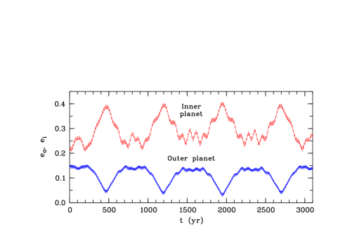
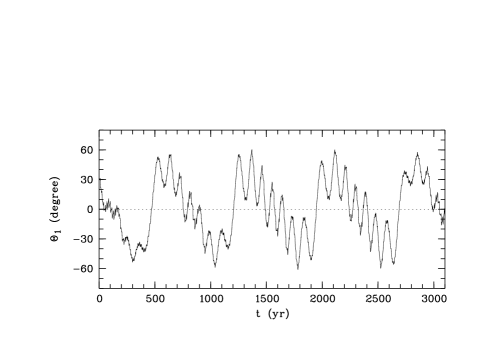
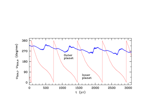
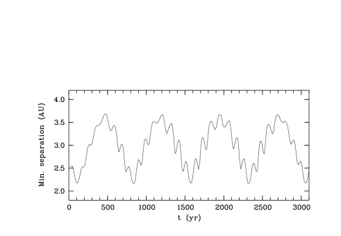
Figure 7: Temporal evolution of selected osculating orbital elements of a model, starting from the best-fit Keplerian parameters of Table 4. The first 3050 yr of the greater than $10^{8}$ yr lifetime are displayed. The left-hand panels show the eccentricities and arguments of periapse for the motion of the center of mass of the binary, the top righthand panel shows the resonant angle $\Theta_{1}$, and the bottom righthand panel the minimum separation between the two planets for successive orbits of the inner planet.

Figure 7 shows the evolution of selected parameters for the best-fitting model of Table 4 over the first 3050 yr of the lifetime, which exceeds $10^{8}$ yr. The two principal periods of the system (Rein & Papaloizou, 2009) are 105 yr and 736 yr. Both are prominent in the librations of $\Theta_{1}$. In the shorter period, low-amplitude anti-phased oscillations of the semi-major axes occur (not shown). In the longer period, $\Delta\omega$ circulates, anti-phased oscillations of the eccentricities take place, and the minimum separation between the two planets reoccurs. The protection mechanism due to the 2 : 1 resonance always keeps the separation above 2.15 AU, effectively limiting the mutual gravitational interaction (bottom right panel). As an illustration, we show the orbits at the time of peak eccentricity $e_{\mathrm{i}}$ in Fig. 8. The system is locked deep in the 2 : 1 mean-motion resonance, as demonstrated by the near-zero mean values of $\Theta_{1}$, averaged over successive 736-yr intervals. For the first 20,000 yr of the evolution, the 26 values of $\langle\Theta_{1}\rangle$ can be represented by an underlying linear and a superposed sinusoidal variation with a period of 3450 yr and an amplitude of $0.86^{\circ}$. The linear component has a fitted slope of $\langle\dot{\Theta}_{1}\rangle\!=\!(-0.2\pm 1.7)\times 10^{-6}$ deg yr^-1, entirely consistent with zero. All long-lived solutions that start from fits in the stability island behave similarly to the best-fit model, in the sense that all of them have $\Theta_{1}$ librating and $\Delta\omega$ circulating. This also holds for the longlived outliers in the central panel of Fig. 3 that have $\tau\!>\!10^{8}$ yr. They differ in the secular period, which ranges from 330 to 1700 yr.

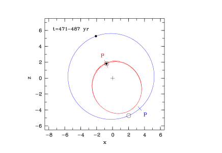
Figure 8: Astrocentric orbits for $t\!=\!471-487$ yr after the begin of the calculation. The locations of the periapses are marked ‘P’, the solid dots indicate conjugation, and the open circles opposition. Orbital motion is counter-clockwise.

All models considered thus far involved prograde coplanar edge-on orbits. We calculated a few models with different inclinations $i_{\mathrm{i}}$ and $i_{\mathrm{o}}$ of the inner and outer planet as a first step toward a more comprehensive study of NN Ser’s planetary system. A common tilt in the planetary orbits, which enhances the planetary masses is limited to $25^{\circ}$, beyond which instability increases rapidly. Similarly, the calculations limited the mutual tilt of the two orbits with respect to each other to $5^{\circ}$.

5 Summary and discussion

We have presented 69 new mid-eclipse times of NN Ser, which cover the minimum and subsequent recovery of the $O\!-\!C_{\mathrm{lin}}$ residuals expected from our previous model in Paper I. The data allowed us to derive a significantly improved two-planet model for NN Ser based on the interpretation of the observed eclipse-time variations in terms of the LTT effect. Combined with extensive stability calculations, we find that the only model that simultaneously fits the data and is secularly stable involves two planets locked in the 2 : 1 mean-motion resonance. We did not find any good fits that are nonresonant and stable. Apart from differences in the periods and mass ratio, the NN Ser system bears resemblance to the HD 128311 planetary system (Sándor & Kley, 2006; Rein & Papaloizou, 2009). The best fit implies eccentricities $e_{\mathrm{o}}\!=\!0.14$ and $e_{\mathrm{i}}\!=\!0.22$ for the outer and inner planets, respectively, and a mass ratio $M_{\mathrm{o}}/M_{\mathrm{i}}\,=\,4$ for coplanar orbits. As expected theoretically for a system with a more massive outer planet (Michtchenko et al., 2008), the temporal evolution of the model that starts from our best fit involves a libration of the resonant variable $\Theta_{1}$ and a circulation of $\Delta\omega$. Preliminary stability calculations for tilted orbits suggest that deviations from coplanarity with the binary orbit cannot be large.

Eclipse-time variations in PCEB seem to be ubiquitous (e.g. Beuermann et al., 2012; Parsons et al., 2010b; Qian et al., 2012, and references therein) and the plausibility of explaining them by the LTT effect has increased by the definitive discovery of planets orbiting non-evolved close binaries with KEPLER (e.g. Doyle et al., 2011; Orosz et al., 2012; Welsh et al., 2012). That the orbital periods in the two types of systems differ by one to two orders of magnitude is a selection effect, because the LTT effect increases with the orbital period, while the radial velocities and transit probabilities decrease. Contrary to radial velocities measured by line shifts, however, the interpretation of the eclipse-time variations in terms of a displacement of the binary along the line of sight is not unique, since eclipse-time variations can also be produced by mechanisms internal to the binary (e.g. Applegate, 1992). Most authors, however, consider this action as inadequate for explaining the magnitude of the observed variations (e.g. Brinkworth et al., 2006; Chen, 2009; Watson & Marsh, 2010). Doubts about the LTT interpretation nevertheless remain, raised by such problematic cases as HU Aqr (Goździewski et al., 2012; Horner et al., 2011; Hinse et al., 2012) and QS Vir (Parsons et al., 2010b). Resolving these cases remains an important task. Presently, NN Ser represents the best documented case in favor of the LTT hypothesis with an agreement between data and model at the 100 ms level, and it is also the prime contender for an observational proof of the required strict periodicity of the signal, given enough time.

The evolutionary history of planetary systems orbiting PCEB may be complex. Planets either existed before the CE and had to pass through the envelope or they were formed in it. In the former case, the orbit of any pre-existing planet is severely affected by the loss of typically more than one half of the mass of the central object. In the latter case, formation depends critically on the conditions in the expanding envelope. In both scenarios, migration may drive a planet pair into resonance, but predicting the properties of the emerging post-CE system is a difficult task. Establishing the structure of systems like NN Ser may provide the observational basis for such a program.