DR 21(OH): a highly fragmented, magnetized, turbulent dense core

Abstract

We present high angular resolution observations of the massive star forming core DR21(OH) at 880 $\mu$m using the Submillimeter Array (SMA). The dense core exhibits an overall velocity gradient in a Keplerian-like pattern, which breaks at the center of the core where SMA 6 and SMA 7 are located. The dust polarization shows a complex magnetic field, compatible with a toroidal configuration. This is in contrast with the large, parsec–scale filament that surrounds the core, where there is a smooth magnetic field. The total magnetic field strengths in the filament and in the core are 0.9 and 2.1 mG, respectively. We found evidence of magnetic field diffusion at the core scales, far beyond the expected value for ambipolar diffusion. It is possible that the diffusion arises from fast magnetic reconnection in the presence of turbulence. The dynamics of the DR 21(OH) core appear to be controlled energetically in equal parts by the magnetic field, magneto–hydrodynamic (MHD) turbulence and the angular momentum. The effect of the angular momentum (this is a fast rotating core) is probably causing the observed toroidal field configuration. Yet, gravitation overwhelms all the forces, making this a clear supercritical core with a mass–to–flux ratio of $\simeq 6$ times the critical value. However, simulations show that this is not enough for the high level of fragmentation observed at 1000 AU scales. Thus, rotation and outflow feedback is probably the main cause of the observed fragmentation.

1. Introduction

DR 21(OH), also known as W75, is a well-studied high-mass star forming region, located inside the Cygnus X molecular cloud complex (Downes & Rinehart, 1966; Motte et al., 2007; Reipurth & Schneider, 2008). It is located in a dense, 4 pc long, DR 21 filamentary ridge, active in star formation, with global infall motions (Harvey et al., 1986; Vallée & Fiege, 2006; Csengeri et al., 2011; Schneider et al., 2010; Hennemann et al., 2012). The distance to the DR21 region has been recently re-estimated through trigonometric parallaxes of masers, $1.50\pm 0.08$ kpc (Rygl et al., 2012), a factor two lower than the previous estimations. We have re-estimated some physical parameters given in previous works taking into account the new distance.

High angular resolution continuum observations show that the DR 21(OH) core is formed by two bright sources, MM 1 and MM 2 (Woody et al., 1989; Lai et al., 2003). But recent subarcsecond angular resolution observations show that these two sources split into a cluster of dusty sources at scales of 1000 AU (Zapata et al., 2012). Chemical analysis of the two main clumps show that MM 1 is more evolved than MM 2 (Mookerjea et al., 2012), which is in agreement with the mid-IR images that show bright emission from MM 1 but no emission toward MM 2 (e.g., Araya et al., 2009). The total bolometric luminosity of DR 21(OH) is $1.6\times 10^{4}$  $L_{\sun}$ (Jakob et al., 2007). DR 21(OH) shows very active and powerful dense outflows, traced not only by CO but also by SiO, CH₃OH, H₂CO and H₂CS (Lai et al., 2003; Minh et al., 2011; Zapata et al., 2012). It also shows a rich variety of masers from molecules such as OH, CH₃OH (class I and II), water and HCO⁺ (e.g., Matthews et al., 1986; Batrla & Menten, 1988; Plambeck & Menten, 1990; Harvey-Smith et al., 2008; Araya et al., 2009; Fish et al., 2011; Hakobian & Crutcher, 2012).

Magnetic fields at large parsec scales have been mapped through single-dish polarimetric observations (Minchin & Murray, 1994; Glenn et al., 1999; Vallée & Fiege, 2006; Kirby, 2009) revealing a relatively uniform magnetic field orientation. Higher angular resolution interferometric observations at millimeter wavelengths (Lai et al., 2003) resolve the magnetic field in the core. Zeeman observations of the CN line reveals a magnetic field strength in the line–of–sight of $B_{\rm los}\simeq 0.4$–0.7 mG (Crutcher et al., 1999).

Polarization observations with the Submillimeter Array (SMA) have been successfully carried out since 2006. In the earlier evolutionary stage of molecular clouds (e.g. collapsing phase), hourglass–like magnetic field lines have been detected in both low–mass star–forming regions (NGC 1333 IRAS 4A, IRAS16293$-$2422: Girart et al., 2006; Rao et al., 2009), and high-mass star-forming regions (G31.41+0.31, W51 e2 and W51 North: Girart et al., 2009; Tang et al., 2009b, 2013), suggesting magnetic–field–regulated gravitational collapses. In contrast, the influences of stellar feedbacks on the magnetic field are seen in more evolved ultra compact HII regions (G5.89$-$0.39, NGC 7538 IRS1: Tang et al., 2009a; Frau et al., 2013) and in the Orion BN/KL region (Tang et al., 2010). Very recently, CARMA has also started to carry out polarimetric observations of dust emission (Hull et al., 2013).

In this paper we present SMA spectro-polarimetric observations carried out at 345 GHz toward DR 21(OH). Here, we focus on the dust polarization observations. Additional data of selected molecular lines are included to better understand the overall properties of this region. Section 2 briefly describes the observations and Section 3 presents the results of the observations. A statistical analysis of the dust polarization is presented in Section 4. Section 5 contains the discussion. Finally, in Section 6 we draw the main conclusions.

2. Observations

The observations were taken with the SMA (Ho et al., 2004) between 2011 June and October in different array configurations. Table 1 lists the observation dates, and for each date the configuration used, the number of antennas, the total amount of time on-source and the polarization calibrators. For all observations but the one from June 30, a single receiver was used around 345 GHz, with a total bandwidth of 4 GHz per sideband. The receiver was tuned to cover the 332.1–336.0 and 344.1–348.0 GHz frequencies in the lower (LSB) and upper sideband (USB), respectively. For the observation on June 30 (in subcompact configuration), the dual–receiver mode was used, tuning the 345 and 400 GHz receivers to the same frequency, which covered the 334.0–335.9 and 344.0–345.9 GHz frequencies in the LSB and USB, respectively. The phase center was $\alpha$(J2000.0)$=20^{\rm h}39^{\rm m}01\fs 20$ and $\delta$(J2000.0)$=$42$\arcdeg 22\arcmin 48\farcs 50$. The correlator provided a spectral resolution of about 0.8 MHz (i.e., 0.7 km s^-1 at 345 GHz) for the single-receiver mode. The gain calibrator was MWC349A. The bandpass calibrator was the same as the polarization calibrator (see Table 1). The absolute flux scale was determined from observations of Ceres and Callisto. The flux uncertainty was estimated to be $\sim 20$%. The data were reduced using the IDL MIR and MIRIAD software packages.

Table 1Observational Parameters

		Number	On-source
Date of		of	Observing	Polariz.
Observations	Configuration	Antennas	Time	Calibrator
2011 Jun 30	Subcompact	7	0.90 hr	3C454.3
2011 Jun 21	Compact	8	0.21 hr	3C279
2011 Jul 13	Compact	7	0.41 hr	3C279
2011 Oct 17	Compact	7	0.78 hr	3C84
2011 Jul 18	Extended	8	0.35 hr	3C454.3
2011 Jul 20	Extended	8	0.35 hr	3C279
2011 Jul 21	Extended	8	0.97 hr	3C279
2011 Jul 23	Extended	8	0.76 hr	3C279
2011 Sep 03	Very extended	8	0.26 hr	3C84

The SMA conducts polarimetric observations by cross-correlating circular polarizations (CP). The CP is produced by inserting quarter wave plates in front of the receivers which are inherently linearly polarized. A detailed description of the instrumentation techniques as well as calibration issues is discussed in Marrone & Rao (2008) and Marrone et al. (2006). We found polarization leakages between 1% and 2% for the USB, while the LSB leakages were between 2% and 4%. These leakages were measured to an accuracy of 0.1% (Marrone & Rao, 2008).

Figure 1.— Visibility coverage of the SMA observations, which includes all the configurations (subcompact, compact, extended and very extended).

Table 2Mapping Parameters

	$u,v$		Synthesized	rms Noise
Configu-	Range	Taper	Beam	Stokes $I$	Pol
ration	k$\lambda$	′′	FWHM, PA	mJy beam-1
SCE	0,90	3.0	$3\farcs 86$$\times$$3\farcs 42$, $56\arcdeg$	20	3.1
SCEV	0,450	0.4	$1\farcs 51$$\times$$1\farcs 21$, $82\arcdeg$	9	1.2
CEV	30,450	0.0	$0\farcs 87$$\times$$0\farcs 65$, $89\arcdeg$	3	1.2

Self-calibration was performed using the Stokes $I$ continuum data for each antenna configuration independently. The derived gain solutions were applied to the molecular line data. The whole data set includes all the different SMA configurations, covering a wide range of visibilities (from 6 up to 450 k$\lambda$). Each configuration is designed to have a relatively uniform density of visibilities. This implies that the combination of several configurations results in a coverage of visibilities with a heterogeneous density (see Figure 1). Therefore, to take advantage of all the information that the whole data contain, maps with different visibility weightings and $u,v$ coverages were used. Table 2 lists the basic parameters of the resulting different maps presented in this paper: $u,v$ coverage, weighting, configuration, synthesized beam, spectral resolution and resulting $rms$ noise. The map at $3^{\prime\prime}$ angular resolution (SCE as defined in Table 2) was made to compare our results with the previous BIMA polarimetric maps (Lai et al., 2003). The map at $1^{\prime\prime}$ angular resolution (Table 2: SCEV) takes advantage of the full visibility coverage at the highest angular resolution and the best sensitivity for the polarization. The subarcsecond map (Table 2: CEV) avoids the larger scale dust emission to trace the magnetic field at scales of few thousands AU. This is done by excluding the shortest baselines. The significantly higher $rms$ noise of the SCEV and CEV Stokes $I$ maps is due to the limited dynamic range of the SMA (the shortest visibilities have strong Stokes $I$ amplitudes). Table 3 gives the transitions, frequency, lower energy level of the molecular lines presented in this paper, as well as the $rms$ noise for channel maps with a velocity width of 1.5  km s^-1. The figures were created using the GREG package (from the GILDAS software).

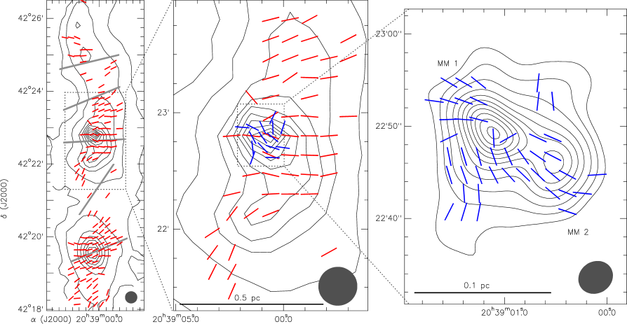
Figure 2.— Left panel: contour map of the dust emission at 850 $\mu$m towards the DR21 region, overlapped with the $B$ segments (red bars) obtained with the JCMT SCUBA polarimeter, SCUPOL (Vallée & Fiege, 2006; Matthews et al., 2009). DR 21(OH) is the brightest core located at the center of the panel. The angular resolution of the map is $20^{\prime\prime}$. Contours are 4%, 8%, 18%,  $\cdots$ , 98% of the peak. Middle panel: zoom-in of the previous panel toward DR 21(OH). The blue bars show the SMA B segments obtained at an angular resolution of $10^{\prime\prime}$. Right panel: contour map of the dust emission at 880 $\mu$m obtained with the SMA (SCE map as defined in Table 2). This panel shows the same map as Fig. 5. Blue bars depict the B segments.

3. Results

In this section we describe the results obtained with the SMA. For the total and polarized dust emission, we also present the single–dish James Clerk Maxwell telescope (JCMT) data obtained with SCUPOL. This allows us to study the magnetic fields from parsec to few thousandths of a parsec scale. Hereafter we define three different physical structures observed at different scales: The DR 21 filament, which is the parsec-long structure where DR 21(OH) is embedded (Vallée & Fiege, 2006); The DR 21(OH) core, a 0.1 pc structure that is resolved into two continuum peaks, MM 1 and MM 2 (Lai et al., 2003) when observed at an arcsecond angular resolution; The substructures detected in the millimeter/submillimeter dust continuum emission maps at scales of 1000 AU (sources SMA 1–9 by Zapata et al., 2012) will be referred as condensations.

3.1. Dust Emission and Magnetic Fields: from Parsec to Sub-parsec Scales

Previous observations have shown that DR 21(OH) is embedded in a 4 pc long dense and massive ($1.5\times 10^{4}$  $M_{\sun}$) filament extending in the north-south direction (Vallée & Fiege, 2006; Hennemann et al., 2012). The filament harbors other star forming cores, such as the well known H II region DR 21 main (Vallée & Fiege, 2006; Hennemann et al., 2012). Figure 2 shows the submillimeter dust emission arising from the filament and the magnetic field that threads the filament. DR 21 main and DR 21(OH) are the bright cores located at the south and at the center of the filament, respectively. The gray long bars shown in this figure represent the average direction of the magnetic field in different sections of the filament. Interestingly, the magnetic field direction in the plane of the sky is close to the East–West direction, and thus almost perpendicular to the filament. The exception is a small region with weak polarization between DR 21(OH) and DR21 main, where the direction flips to a position angle of $\simeq$146°. The variation of the direction along the filament occurs smoothly. Around DR 21 main the magnetic field configuration is compatible with the hourglass morphology (Kirby, 2009). There are other reports of massive filaments with magnetic fields perpendicular to the filament (e.g., G14.225, Busquet et al., 2013).

The zoom–in of the single–dish polarization map toward the filament around DR 21(OH)  (the middle panel of Figure 2, red bars) shows that the magnetic field is relatively uniform and mostly in the east-west direction. This pattern of the magnetic field is in agreement with CO J=2-1 and 1-0 polarimetric data derived with BIMA (Lai et al., 2003; Cortes et al., 2005), which trace the low density molecular gas, $n({\rm H}_{2})\simeq 10^{2}$  cm^-2. In contrast, the SMA polarization map at an angular resolution of $3^{\prime\prime}$ reveals field orientations much less uniform (see the right panel of Figure 2). To properly compare the SMA and SCUBA polarization maps, we convolved the $3^{\prime\prime}$ SMA map with a Gaussian to degrade the angular resolution up to $10^{\prime\prime}$. The resulting map, shown in the central panel of Figure 2, reveals that the magnetic field derived from the SMA at this angular resolution (blue segments in this figure) is still less uniform, even though some of the magnetic field segments are roughly aligned in the E-W direction, the direction of the filament component. It is important to remark that the SMA filters out the large-scale component from the dust total and polarized intensity. Therefore, the SMA is more sensitive to the small-scale magnetic field within the core, whereas the single-dish map is more sensitive to the total column density of dense molecular gas, thereby to the large-scale component. We, thus, do not necessarily expect to recover the SCUBA field morphology after convolving the SMA data.

3.2. Dust Emission and Magnetic Fields: from 20,000 to 1000 AU Scales

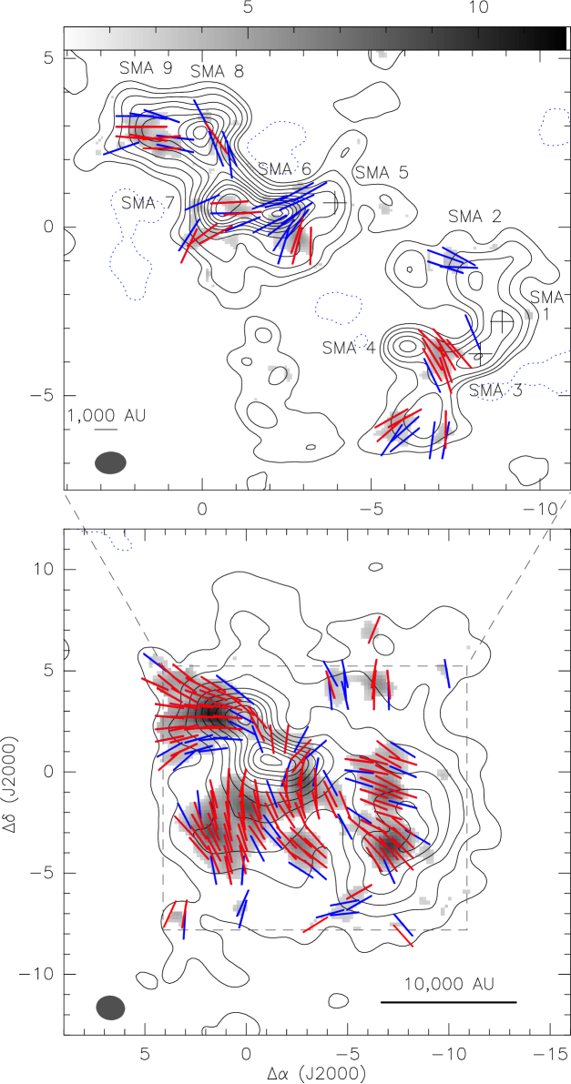
Figure 3.— Contour map of the dust emission at 880 $\mu$m, overlapped with the gray scale intensity of the dust linear polarized emission and the B segments. Bottom panel: Images with an angular resolution of $\simeq 1\farcs 3$ obtained using all the configurations (SCEV map as defined in Table 2). Top panel: Images with an angular resolution of $\simeq 0\farcs 75$ obtained using all the configurations but the subcompact one (CEV map as defined in Table 2). The red and blue segments show the magnetic field segments with a significance level of $\gtrsim 3$–$\sigma$ and between 2.5 and 3 $\sigma$, respectively. The synthesized beam is shown in the bottom left corner of each panel. Contours in the two panels are 5%, 10%, 17%, 27%,  $\cdots$ , 97% of the peak, 0.85 and 0.29 Jy beam^-1 for the $1\farcs 3$ and $0\farcs 75$ angular resolution maps, respectively.

Observations at an angular resolution of $3\farcs 6$ ($\simeq 5500$ AU, see Figure 5) show that the millimeter continuum emission is dominated by the dust emission and arises from two main components, MM 1 and MM 2 (Woody et al., 1989; Lai et al., 2003). However, the higher angular resolution map reveals clearly how this region fragments in a significant way. First, the map obtained using all the visibilities and with an angular resolution of $\simeq 1\farcs 3$ (configuration SCEV from Table 2; see also the bottom panel of Figure 3) shows that MM 1 has split into two bright components, whereas MM 2 appears elongated with an arc-like morphology. The fragmentation is more evident at sub–arcsecond scales ($\simeq 1000$ AU, as shown in the top panel of Figure 3) for a map obtained excluding the shortest baselines ($r_{\rm u,v}<30$ k$\lambda$), and thereby filtering some of the extended component that appears in the $\simeq 1\farcs 3$ map. At this angular resolution, the 880  $\mu$m map is in agreement with the 1.4 mm map obtained by Zapata et al. (2012), although the better sensitivity allows us to detect more emission. MM 1 splits into four bright sources (from west to east, SMA 6, SMA 7, SMA 8 and SMA 9, according to Zapata et al. 2012 nomenclature). SMA 5 is not well resolved at this angular resolution. SMA 6 and SMA 7 are the sources located closer to the center of the whole dense molecular core. MM 2 splits in several components: a compact source SMA 4, an elongated structure that contains SMA 1, SMA 2 and SMA 3, and possibly two additional components not previously reported: one $2^{\prime\prime}$ south of SMA 4 and the other $2^{\prime\prime}$ east of SMA 2. In brief, DR 21(OH) splits probably in more than 10 sources and this constitutes an extreme case of a highly fragmented dense molecular core, according to a recent study carried out at similar spatial scales over a sample of 18 intermediate and massive dense cores (Palau et al., 2013).

The total flux measured at 880 $\mu$m is $18.8\pm 0.1$ Jy. To estimate the mass we adopt a gas-to-dust ratio of 100 and a dust opacity of 1.5 cm² g^-1, which is approximately the expected value for dust grains with thin dust mantles at densities of $\sim 10^{6}$   cm^-3 (Ossenkopf & Henning, 1994). Assuming a temperature of 30 K (Mayer et al., 1973; Vallée & Fiege, 2006), we then estimate the total mass traced by the dust to be 150  $M_{\sun}$. This value is a factor of 2 lower than the mass derived from single–dish measurements of the dust emission (350  $M_{\sun}$: Motte et al., 2007), which is likely due to the filtering effect of the SMA. To derive the averaged volume and column densities in the whole DR 21(OH) core, we use the full width at half maximum (FWHM) of the dust emission at an angular resolution of $3^{\prime\prime}$, FWHM$\simeq 10\farcs 4$. This value yields an average column and volume density of $1.6\times 10^{24}$  cm^-2 and $1.0\times 10^{7}$  cm^-3, respectively.

Figure 4 shows the distribution of the angles of the magnetic field segments measured in the $1\farcs 3$ angular resolution map with a Nyquist sampling and with a cutoff in the polarized emission of 3–$\sigma$. The distribution shows a broad dispersion in the 0 to 80° range without a clear main direction. However, a visual inspection of the resulting magnetic field (see bottom panel of Figure 3) seems to show that there are two main directions of the magnetic field: (1) NE–SW around MM 2 and east of MM 1 and (2) N–S in the northern part of the dense core and South of MM 1. It is interesting to note that most of the intensity peaks, with the exception of SMA 7 and SMA 9, devoid the polarized intensity.

Figure 4.— Distribution of position angles of the magnetic field segments shown in the $1\farcs 32$ angular-resolution map for a polarized emission cutoff of 3.0–$\sigma$.

The subarcsecond angular resolution map shows that most of the dust polarized emission is resolved out, specially the N–S component. This suggests that this component arises from the resolved–out core that surrounds the compact condensations. The polarized emission that traces the NE–SW magnetic field component is partially detected towards MM 2 and MM 1-SMA 9. Surprisingly, the higher angular resolution map shows polarized emission around SMA 7, which was undetected in the lower angular resolution maps. This is probably due to the beam smearing: with a larger beam, SMA 7 will have contributions of different field directions, which cancel out in the Stokes $Q$ and $U$ maps, because they would have different signs. The magnetic field directions in the SMA 6–7 cores appear to be oriented in the E-W direction, with the field bending to a north–south direction South of these cores. Most of MM 2 appears unpolarized at the present sensitivity.

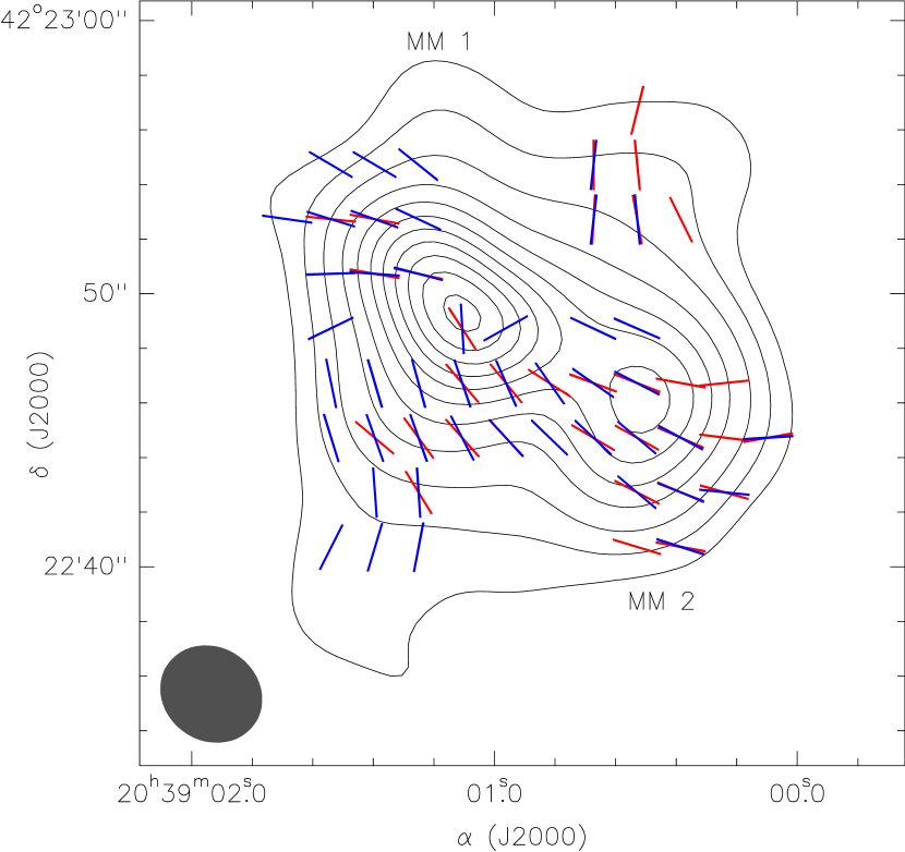
Figure 5.— Contour map of the SMA dust emission at 880 $\mu$m. The map was obtained from the combined data of the subcompact, compact and extended configurations with a Gaussian taper to match the BIMA polarization maps by Lai et al. (2003). The synthesized beam is shown in the bottom left corner of the panel. Overlapped with the contour maps are the B segments derived at a similar angular resolution by BIMA (red segments; from Lai et al. 2003) and the SMA (blue segments).

3.2.1 Comparison with Previous BIMA Observations

Figure 5 shows the 880 $\mu$m continuum emission of the total intensity (Stokes $I$) and the magnetic fields (B) segments from the SMA combined data as well as from BIMA obtained at 1.3 mm by Lai et al. (2003). At these two wavelengths the continuum emission is dominated by the dust emission (Lai et al., 2003). The SMA dust continuum map shows a remarkably similar morphology to the 1.3 mm BIMA map (see Figure 7 from Lai et al. 2003), resolving clearly MM 1 and MM 2. The SMA detects slightly more linearly polarized dust emission than BIMA. This is because the dust emission at 880 $\mu$m is significantly brighter than at 1.3 mm, whereas the sensitivity and the polarization fraction are similar at both wavelengths. Yet, the overall pattern is also quite similar. The largest differences appear South of MM 1, where the B segments in the BIMA data are oriented in the SE–NW direction, whereas the SMA data are oriented more toward the E-W direction (see Figure 1 from Lai et al. 2003 and Figure 5 from this paper). Indeed, the average difference between the polarization angles of the two arrays in the SE–NW region is $\Delta PA$=$20$°$\pm 12$°, whereas in the rest of the region the difference is only $7$°$\pm 5$°.

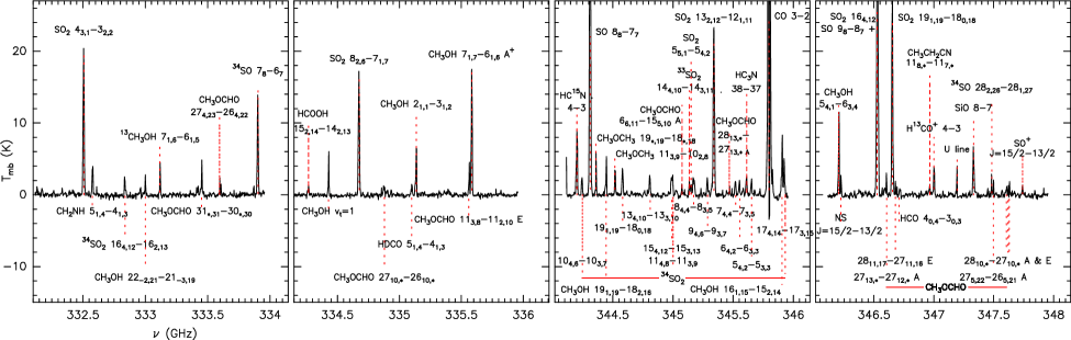
Figure 6.— Averaged spectra over an area of $\simeq 4$ arcsec² around SMA 6 and SMA 7. The spectra were derived using the compact, extended and very extended configurations with a natural weighting which yields a synthesized beam of $1\farcs 4\times 1\farcs 1$ and PA=83°.

3.3. Molecular Lines: Dense Core Chemical Content

Table 3Molecular line parameters

			rms	Synthesized
Molecular	$\nu$	$E_{\rm L}$	(Jy/	beam
Transition	(GHz)	(K)	Beam)	FWHM (′′), PA
CO 3–2	345.796	17	0.10	0.91$\times$0.66, 89°
HC15N 4–3	344.200	25	0.09	1.79$\times$1.64, 62°
H13CO+ 4–3	346.998	25	0.12	1.80$\times$1.63, 61°
CH3OCH3 113,9–102,8	344.358	56	0.09	0.90$\times$0.67, $-88$°
CH3CH2CN 258,17–257,18	333.120	194	0.08	0.89$\times$0.67, 89°
CH3OH 182,16–173,14	344.109	403	0.09	0.90$\times$0.67, $-88$°

The SMA observations sample a total of 7.8 GHz bandwidth at a spectral resolution of 0.6 km s^-1. They, therefore, capture many lines in the 880 $\mu$m band. The emission of most of these lines appears to be compact and mostly associated with SMA 6, SMA 7 and to a smaller extent with SMA 4. The spectra toward SMA 6 and SMA 7 (see Figure 6) clearly show that they are dominated by hot–core line tracers such as methanol (CH₃OH), sulfur monoxide and dioxide (SO and SO₂) and methyl formate (CH₃OCHO). There are also other hot-core tracers: oxygen–bearing species, such as dimethyl ether (CH₃OCH₃) and formic acid (HCOOH); nitrogen-bearing species, such as cyanoacetylene (HC₃N), nitrogen monosulfide (NS), methanimine (CH₂NH) and ethyl cyanide (CH₃CH₂CN) . The “exotic” sulfur monoxide ion (SO⁺) is also detected, which is a diagnostic of dissociative shock chemistry (Turner, 1992). There is an unidentified line at 347.191 GHz, which has been previously reported toward Orion KL/IRc2 (Jewell et al., 1989). There are other molecular species that exhibit more extended emission, tracing either the whole DR 21(OH) dense core (HC¹⁵N, H¹³CO⁺) or the powerful outflow (CO, SiO). A more detailed study of the complete molecular content detected with this set of observations will be reported in a forthcoming paper. In this paper, we focus on a selected set of lines in order to better understand the kinematic characteristics of the core, the SMA 6 and SMA 7 condensations and of the outflows, which in addition are useful to better understand the complex magnetic field configurations. Table 3 shows the list of molecules used in this paper, with the selected transition, rest frequency, lower energy level, $rms$ noise level and the angular resolution.

3.4. Molecular Lines: Tracing the Gas Kinematics

Figure 7 shows the integrated emission of the H¹³CO⁺ 4–3 line, as well as its first order moment (the velocity field) overlapped with the dust emission at a similar angular resolution. H¹³CO⁺ is about $\sim 90$ times less abundant than H¹²CO⁺, and it is optically thin (Hezareh et al., 2010). The 4–3 line has a critical density of $\sim 10^{7}$  cm^-3, which is similar to the averaged density found from the dust continuum observations (see Section 3.2). All these characteristics indicate that this molecular transition is, thus, a good tracer of the very dense, warm core. Indeed, the integrated emission appears to trace remarkably well the dust emission. The main difference between the dust and H¹³CO⁺ emission is toward the condensations SMA 6 and SMA 7, where the H¹³CO⁺ emission does not show a peak as the dust emission. This suggests that this line does not trace the hot core–like condensations.

Figure 7.— Top panel: gray scale image of the H¹³CO⁺ 4–3 integrated emission overlapped with the contour map of the dust emission at an angular resolution of $1\farcs 3$. Bottom panel: color image of the H¹³CO⁺ 4–3 first–order moment (intensity weighted mean  $v_{\rm LSR}$) overlapped with the contour map of the dust emission. The wedge units are in  km s^-1.

The flux-weighted velocity map of the H¹³CO⁺ 4–3 line shows a clear velocity gradient along the NE–SW direction, which roughly coincides with the major axis of the dense envelope and one of the magnetic field dominant directions. This velocity pattern agrees with the velocity pattern in the filament around the core, as traced by the lower density lines H¹³CO⁺ 1–0 and N₂H⁺ 1–0 (Schneider et al., 2010). A cut along the major axis of the DR 21(OH) dense envelope (PA=$63$°; see the top panel of Figure 8) shows clearly this velocity gradient. The eastern side of the envelope is blue-shifted with respect to the western side, with systemic velocities of  $v_{\rm LSR}$ $\simeq-4.7$  km s^-1 and  $v_{\rm LSR}$ $\simeq-2.3$  km s^-1, respectively. Using as a reference the distance between the eastern and western edges of the envelope along the major axis (i. e., along the NE–SW direction), $\simeq 20^{\prime\prime}$, and the observed velocity difference between these two edges, $\simeq 2.4$  km s^-1, we estimate a velocity gradient over the whole core of $\simeq 18$  km s^-1 pc^-1. At about $4^{\prime\prime}$ (5600 AU in projection) from SMA 6 the gas velocity starts to increase in a Keplerian–like motion (i. e., the blueshifted/redshifted gas becomes bluer/redder toward the center). However, the lack of H¹³CO⁺ 4–3 emission associated with the SMA 6–7 condensations does not allow us to inspect the kinematics at the very center.

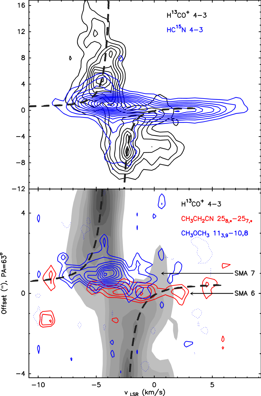
Figure 8.— Plot of the velocity vs. position map for a position angle of $PA=63\arcdeg$ along the major axis of the DR 21(OH) dense core. The 0^′′ position is at the location of the SMA 6 hot core (RA$=20^{\rm h}39^{\rm m}1\fs 00$ of and DEC$=42\arcdeg 22^{\prime}48\farcs 93$). Top panel: H¹³CO⁺ (black solid lines) and HC¹⁵N (blue solid lies) lines. Bottom panel: H¹³CO⁺(gray scale), dimethyl ether (blue contours) and ethyl cyanide (red contours). The specific transitions are shown in the top right corner of each panel. The dashed thick line shows the expected Keplerian rotation.

In order to check the kinematics at the center of the core, we have made maps of four different molecular lines (see Table 3). The HC¹⁵N 4–3 emission is similar to H¹³CO⁺ 4–3 but slightly more compact and brighter toward SMA 6–7. The position-velocity cut of the HC¹⁵N line along the major axis is similar to the H¹³CO⁺ line at scales of few arcseconds. However, there are significant differences between these two tracers at distances less than $\lesssim 1\farcs 5$ ($\lesssim 2000$ AU) from the center. The HC¹⁵N line is much brighter and its emission arises from two components that are not traced by the H¹³CO⁺line: one at $-4$  km s^-1, associated with SMA 7, and another one at 2  km s^-1 arising from SMA 6. These two components appear to break the Keplerian–like kinematic behavior observed in the H¹³CO⁺ line. To further investigate the kinematics around the densest part of the DR 21(OH) center, SMA 6 and SMA 7, Figure 9 shows the first-order moment maps of three hot-core molecular transitions, overlapped with the dust continuum maps. All of them are obtained at a sub-arcsecond angular resolution. The CH₃OH line – which has a high excitation energy level – traces very well the two hot cores SMA 6 and SMA 7. The velocity behavior resembles well the one from the HC¹⁵N line, particularly the red-shifted component at 2  km s^-1 associated with SMA 6. The dimethyl ether line emission traces only SMA 7, which is observed in both CH₃OH and HC¹⁵N  lines with a systemic velocity of $-4$  km s^-1. This line shows a velocity gradient of $\simeq 1$  km s^-1 roughly along the SMA 7 major axis, i. e., along the NW-SE direction. On the other hand, the ethyl cyanide line traces only the dense gas associated with SMA 6. It also shows a small velocity gradient of 1  km s^-1 but along the E-W direction. Interestingly, the line peaks at a  $v_{\rm LSR}$ velocity of $\simeq-2$  km s^-1. This is quite different from the CH₃OH  and the HC¹⁵N line emission around SMA 6 (see the top panel of Figure 8). The bottom panel of Figure 8 shows the position-velocity cuts for the dimethyl ether and ethyl cyanide overlapped with the H¹³CO⁺. As already shown by HC¹⁵N, the gas traced by these two hot-core lines apparently does not follow the Keplerian–like behavior of the H¹³CO⁺ emission. In Section 5 we discuss the interpretation of these differences.

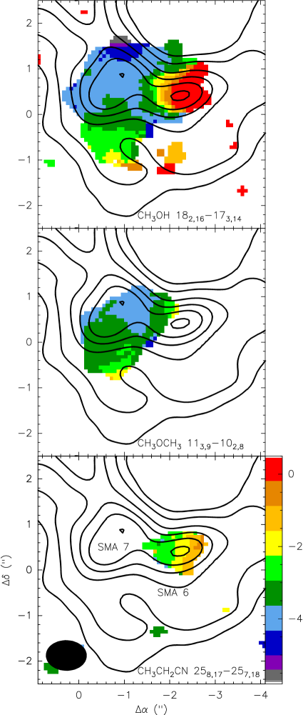
Figure 9.— Contour maps of the sub-arcsecond angular resolution dust emission overlapped with the color images of the first-order moment maps of three selected molecular transitions. The wedge units are in  km s^-1. Top panel: CH₃OH 18_2,16–17_3,14; Middle panel: CH₃OCH₃ 11_3,9-10_2,8; Bottom panel: CH₃CH₂CN 25_8,17–25_7,18.

3.5. CO 3–2: A Molecular Outflow Tracer

Figure 10 shows the high-velocity (HV) emission of the CO 3–2 line at an angular resolution of $\simeq 1^{\prime\prime}$ for two different velocity ranges in the blue and red lobes. The overall pattern agrees with the previous lower angular resolution BIMA interferometric maps ($\simeq 5^{\prime\prime}$) of the CO 2–1 line by Lai et al. (2003). The CO 2–1 maps showed two bipolar outflows oriented roughly in the E–W direction with the red-shifted lobes in the eastern part. The SMA CO 3–2 maps show that most of the emission is distributed similarly to the CO 2-1 emission, but the higher angular resolution reveals a more complicated morphology. The extremely high–velocity (EHV) CO emission (velocities from 40 to 90  km s^-1  with respect to the cloud velocity) appears to arise from a bipolar structure with a position angle in the direction of the red-shifted lobe of about 110°. The origin of the outflow appears to be in MM 2, possibly from SMA 3 or SMA 4. At HVs (velocities from 20 to 40  km s^-1 with respect to the cloud velocity) there are two highly collimated bipolar outflows with position angles of 95°and 65°. The first one appears to also arise from MM 2, possibly SMA 4, although we cannot discard source SMA 3. It is possible that this HV emission is part of the same outflow as the EHV bipolar component, as suggested from methanol and formaldehyde observations (Zapata et al., 2012). The second outflow arises from MM 1, possibly from SMA 6 or SMA 7. There is an isolated redshifted clump only $2^{\prime\prime}$ away of SMA 6 and 7, without a blue-shifted counterpart in the same velocity range. It is very close to a compact, low velocity outflow detected in H₂CS (Minh et al., 2011).

Interestingly, the interferometric maps of the CO 3–2 outflows are strikingly different from the single-dish maps of the same transition (Vallée & Fiege, 2006). These lower angular-resolution ($\sim 14^{\prime\prime}$) maps show a low-velocity outflow with a position angle of roughly 130°, with the blue and red lobes located NW and SW, respectively, of the DR 21(OH) center. This low-velocity outflow is not seen in the SMA maps because it is probably too extended, and therefore most of the emission is filtered out.

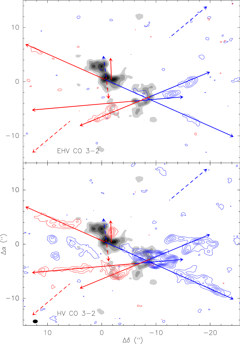
Figure 10.— Maps of the red-shifted (red contours) and blue-shifted (blue contours) emission of the CO 3–2 line. Top panel: EHV component obtained by averaging the emission over 50  km s^-1 centered at a velocity $\pm 65$  km s^-1 with respect to the system velocity of the DR 21(OH) core,  $v_{\rm LSR}$ $\simeq-3$  km s^-1. Bottom panel: HV component obtained by averaging the emission over 20  km s^-1 centered at a velocity $\pm 30$  km s^-1 with respect to the system velocity. The gray-scale map shows the dust continuum image of the high-angular resolution. The synthesized beam of the CO maps is shown in the bottom left corner of the bottom panel. Solid arrows show the observed outflows in the CO 3–2 maps. Dashed arrows show the bipolar outflows detected previously by Minh et al. (2011) from the SMA H₂CS observations (compact N–S arrows centered around SMA 6–7) and Vallée & Fiege (2006) from single-dish observations of CO 3–2 (SE–NW arrows).

4. Analysis: Statistical derivation of the magnetic field strength

Figure 3 shows clearly that at the scales traced by the SMA, the magnetic field segments in the DR 21(OH) region do not follow a defined homogeneous pattern as, e.g., the hourglass shape reported in some low- and high-mass star-forming cores (Girart et al., 2006, 2009). However, if we take into account the large-scale polarization maps, the magnetic field segments show significant coherence in all the maps except the one tracing the densest regions. No simple analytical models are available to be compared with this complex magnetic field and mass distribution (see, e.g., Frau et al., 2011). Therefore, in order to extract physical information, a statistical approach seems to be the best available option.

To statistically analyze the data we have estimated the angular dispersion function, 1–$<$cos$[\Delta\Phi(l)]$$>$, where $\Delta\Phi(l)$ is the difference between the polarization angles measured for all pairs of points separated by a distance $l$. Note that for small values of $\Delta\Phi(l)$, 1–$<$cos$[\Delta\Phi(l)]$$>\simeq 1/2$$<$$\Delta\Phi^{2}(l)$$>$, which is the second–order structure function of the polarization angles. This function gives information on the behavior of the dispersion of the polarization angles as a function of the length scale in the dense molecular gas (Hildebrand et al., 2009; Houde et al., 2009, 2011; Franco et al., 2010; Koch et al., 2010). Figure 11 shows this function applied to the SMA and SCUPOL polarimetric data (the top and bottom panels, respectively). For the two telescopes, due to the effect of the limited angular resolution, the angular dispersion function is zero at $l=0$ and then smoothly increases with the length scale. However, the overall behavior is quite different between the two telescopes. On one hand, in the SMA polarization data the second order dispersion function increases with angular separation $l$, reaching values compatible with a random magnetic field ($\simeq$52°: Poidevin et al., 2010) at scales of $4^{\prime\prime}$ (5600 AU). This behavior is similar to the one found in NGC 7538 IRS 1 (Frau et al., 2013). Interestingly at scales larger than $8^{\prime\prime}$ ($10^{4}$ AU), the angular dispersion starts to decrease to values of $\simeq 0.2$ (this is equivalent to an angular dispersion of $\sim 35$°). On the other hand, the SCUPOL data, which traces much larger scales than the SMA ($\gtrsim 20^{\prime\prime}$), shows that the dispersion never reaches the value expected for a random field. Indeed, the maximum angular dispersion at $l=100^{\prime\prime}$ ($10^{5}$ AU) is roughly 0.2.

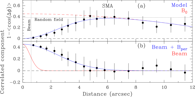
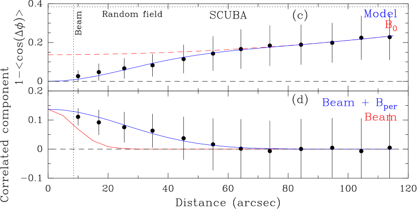
Figure 11.— Panels (a) and (c): angular dispersion function using the magnetic field segments detected towards DR 21(OH), obtained using a Nyquist sampling. The data points (shown as dots) and the error bars are the mean and standard deviation of all the pairs contained in each bin. The red dashed line shows the fitted $f_{{\rm NC}}(0)\,+a^{\prime}_{2}\,l^{2}$. The dotted vertical line gives the FWHM of the synthesized beam. The dotted horizontal line shows the expected value for a random magnetic field. The blue line shows the best fit to the data (Equation (1)). Panels (b) and (d): the dots represent the correlated component of the best fit to the data. The dashed line marks the zero value. The solid red line shows the correlation due to the beam, and the blue line shows the correlation due to the beam and the turbulent component of the magnetic field. Panels (a) and (b) show the data from SMA. Panels (c) and (d) show the data from SCUBA.

Table 4Angular Dispersion Function Fit Parameters

Parameter	SMA	SCUPOL
$\delta$ (mpc)	$16.9\pm 1.6$	$151\pm 21$
$f_{{\rm NC}}(0)$	$0.45\pm 0.04$	$0.137\pm 0.015$
$\Delta^{\prime}$ (pc)	$\simeq 0.08$	$0.34$
$n({\rm H_{2}})$ (cm-3)	$1.0\times 10^{7}$	$2.0\times 10^{5}$
$\delta V$ (km s-1)	1.0	0.8
$\langle B^{2}_{\rm t}\rangle/\langle B^{2}_{0}\rangle$	$\simeq 0.92$	$\simeq 0.16$
$\langle B\rangle_{pos}$ (mG)	$\simeq 2.1$	$\simeq 0.62$
$\langle B\rangle$ (mG)	$\simeq 2.1$	$\simeq 0.9$4

Assuming a stationary, homogeneous, and isotropic magnetic field strength and a magnetic field turbulent correlation length, $\delta$, smaller than the thickness of the cloud $\Delta^{\prime}$, Houde et al. (2009) have shown that the angular dispersion function can be used to estimate the importance of the magnetic field. We have used Equation (42) from Houde et al. (2009), which takes into account the smearing effect of the beam and the line-of-sight integration, to estimate the importance of the field. Under these assumptions, the dispersion function can be rewritten as

$$1-\langle\cos\left[\Delta\Phi\left(\,l\,\right)\right]\rangle\simeq f_{{\rm NC}}(0)\,\left[1-e^{-l^{2}/2(\delta^{2}+2W^{2})}\right]\\ +\sum^{\infty}_{j=1}a^{\prime}_{2j}\,l^{2j},$$ (1)

where $l$ is the length scale and $W$ is the beam “radius”. The summation on the right hand side of the equation is the contribution from the ordered component of the magnetic field, and $f_{{\rm NC}}(0)$ is the value of the correlated component at the origin (shown in the bottom panel of Figure 11). This value depends on the energy ratio between the turbulent or perturbed magnetic field and the ordered large-scale magnetic field, $\langle B^{2}_{\rm t}\rangle/\langle B^{2}_{0}\rangle$, and the number of independent turbulent cells contained in the column of dust probed observationally, $N$: $f_{{\rm NC}}(0)=(\langle B^{2}_{\rm t}\rangle/\langle B^{2}_{0}\rangle)\,(1/N)$. According to Houde et al. (2009),

$$N=\Delta^{\prime}\,(\delta^{2}+2W^{2})/(\sqrt{2\pi}\delta^{3})$$ (2)

where $\Delta^{\prime}$ is in the effective thickness of the molecular cloud, which is expected to be somewhat smaller than the cloud thickness.

4.1. SMA Polarization Data

In the case of the SMA polarization data, Figure 11 shows that at scales larger than $l\sim 4^{\prime\prime}$, the magnetic field has statistically values similar to what is expected for a random field (though for $l\gtrsim 8^{\prime\prime}$ the dispersion function decreases below the random field value). However, this does not imply that the magnetic field is random (see Section 5 for a discussion on this issue). The best fits to the SMA DR 21(OH)  polarimetric data (see Table 4 and the top two panels of Figure 11) lead to a turbulent magnetic field correlation length of $\delta=2\farcs 33\pm 0\farcs 22$ ($16.9\pm 1.6$ mpc at 1.5 kpc). The derived value of the correlated component at the origin is $f_{{\rm NC}}(0)$ $\simeq 0.45$. A reasonable approximation is to assume that the core’s effective thickness, $\Delta^{\prime}$ is similar to the average diameter of the dense core measured in the plane of the sky with the SMA (Koch et al., 2010), which in our case is $\simeq 10\farcs 4$ ($\sim 1.6\times 10^{4}$ AU, see Figure 3). Following Equation (2), this yields to $N\simeq 2$ turbulent cells along the line-of-sight. This implies that $\langle B^{2}_{\rm t}\rangle/\langle B^{2}_{0}\rangle\simeq 1$, i. e., there is equipartition between the perturbed and ordered magnetic field energies.

The Chandrasekhar–Fermi (CF) equation can be used to derive the magnetic field strength in the plane of the sky, $\langle B^{2}_{0}\rangle^{1/2}\propto\delta V\,n({\rm H_{2}})^{1/2}\left[\langle B^{2}_{\rm t}\rangle/\langle B^{2}_{0}\rangle\right]^{-1/2}$ (e.g., see Equation (57) by Houde et al., 2009). Table 4 shows the values used for the velocity dispersion, $\delta V$, and for the volume density, $n({\rm H_{2}})$. We estimated the velocity dispersion from the H¹³CO⁺ 4–3 data, since, as shown in section 3.3, its emission is well correlated with the 880 $\mu$m dust emission. For the volume density, we used the value derived in Section 3.2. From the combination of both results, the ordered large-scale magnetic field strength component in the plane-of-sky, $\langle B^{2}_{0}\rangle^{1/2}$, $\simeq 2.1$ mG.

4.2. JCMT-SCUPOL Polarization Data

For the SCUPOL, we follow the same steps of the previous subsection. However, we only compute the statistics for length scales less than $2\farcm 0$, since we want to fit the scales in Figure 11 where the ordered, large-scale component is approximately linear. The physical parameters derived from the analysis are shown in the right column of Table 4. The turbulent correlation length is about 0.15 pc which is significantly larger than for the SMA. The derived value of $f_{{\rm NC}}(0)$ is $\simeq 0.14$. For the effective thickness we adopt the value of the filament width obtained from Herschel observations, 0.34 pc (Hennemann et al., 2012). Using the velocity dispersion and the volume density values reported in the literature for the filament, we derive a perturbed-to-ordered magnetic energy ratio significantly lower than the value for the DR 21(OH) core, $\simeq 0.2$. The plane-of-the-sky magnetic field strength is 0.62 mG, similar to the value derived previously (Vallée & Fiege, 2006).

5. Discussion: The relevance of the magnetic fields

5.1. Comments on Individual Sources

It is noteworthy that most of the dust peaks of the different condensations (Figure 3) are devoid of polarized emission. This can be due to beam cancellation at the center of the different condensations, where gravity pulls the field lines to the center (Frau et al., 2011). Of the different submillimeter condensations, only three, namely SMA 4, SMA 6 and SMA 7 show clear signs of on–going star formation.

SMA 4 has a very compact dust distribution, and it has associated emission from shock-excited dense tracers. In addition, it appears to be the powering source of the east-west highly collimated CO outflow. The strong methanol and formaldehyde emission associated with this outflow (Zapata et al., 2012) suggests that this outflow is strongly interacting with the dense gas.

With a mass of $\simeq 23$  $M_{\sun}$ (Zapata et al., 2012), SMA 6 is one of the most massive condensations embedded in the DR 21(OH) core near the geometrical center of the core. A very compact and dense molecular outflow has been detected in the N–S direction that appears to be centered on this source (Minh et al., 2011). The SMA observations show that it has a hot–core like chemistry. The ethyl cyanide, a hot-core tracer, is present only in this source (the bottom panel of Figure 9). This tracer shows a clear velocity gradient along the east–west direction, i. e., perpendicular to the associated compact outflow. Thus, this velocity gradient probably indicates rotation. The red–shifted component seen in methanol and HC¹⁵N (Figures 8 and 9) is likely tracing shock–excited emission from the compact outflow.

SMA 7 is the other massive condensation with a mass similar to SMA 6. It also has a hot–core chemistry, although it is different with respect to SMA 6 (J. M. Girart, private communication). For example, dimethyl ether is only detected in this source (see the middle panel of Figure 9). Its emission appears to be extended in the NW–SE direction, with a velocity gradient along the same direction. This velocity gradient is roughly perpendicular to the highly collimated CO outflow with PA=65°. This suggests that SMA 7 is the powering source of this outflow. Both SMA 6 and SMA 7 have velocity gradients that does not match the large scale velocity gradient seen in the core through the H¹³CO⁺ 4–3 emission. Recent simulations of non-idealized magnetized massive cores show that turbulence can generate the observed misalignment (Seifried et al., 2012).

5.2. Interpretation of the Statistical Analysis

The polarization angle dispersion shows relatively high values for the SMA observations, as high as those expected for a random field. However, this does not imply that there is a lack of an ordered field. As an example, the classical ordered hourglass magnetic field expected in a magnetized core with little turbulence and rotation – which has been observed in some protostars (Girart et al., 1999, 2006; Lai et al., 2002; Alves et al., 2011) – will have a radial pattern in the plane of the sky in the case of a face–on configuration (Frau et al., 2011; Padovani et al., 2012; Kataoka et al., 2012). A similar case would be a toroidal field (due to rotation) also face–on. Both patterns would also appear in the structure function with values close to the ones expected for a random field. For a qualitative assessment, we have computed the second-order structure function on the simulations shown in the two bottom panels of Figure 8 by Padovani et al. (2012). These two panels show the B segments of a toroidal magnetic configuration seen face–on at two different times of the collapse of a magnetized core using the RAMSES code (Fromang et al., 2006; Hennebelle & Fromang, 2008; Hennebelle & Ciardi, 2009). Despite that the conditions are different (the simulations used are for a low mass star forming core), we found that the overall statistical trend of the toroidal field simulations confirm that the second-order structure function behavior observed in the SMA data can be explained simply by a toroidal field (see Section 5.6) rather than a very turbulent medium.

The statistical analysis carried out with the SMA polarimetric data toward DR 21(OH) yields values of the turbulent length scale, $\simeq 17$ mpc, and of the magnetic field strength component in the plane of the sky, $\simeq 2.1$ mG, that is in very good agreement with the values derived from a completely independent method by Hezareh et al. (2010) who found 9 mpc and 1.7 mG. They computed these values from the correlation of the velocity dispersion of the coexisting neutral and ionized species H¹³CN and H¹³CO⁺, using their rotational 4–3 line. Note that as stated previously, our SMA data show that the H¹³CO⁺ 4–3 correlates well with the 880 $\mu$m dust emission, i. e., they trace the same gas. This good agreement gives confidence in the values derived despite the uncertainties of the analysis method. Furthermore, the value of the correlation length derived with the SMA is also within a factor of two of the values reported in the literature for interferometric observations of three other massive star forming regions, W51, Orion KL/Irc2 and NGC 7538 IRS1 (Koch et al., 2010; Houde et al., 2011; Frau et al., 2013).

The analysis done with SCUPOL gives a correlation length scale significantly larger than the value found with the SMA. However, the field strength (in the plane of the sky) is similar to the value derived by Vallée & Fiege (2006) who were using directly the C-F method.

5.3. Turbulence versus Magnetic Fields

The line width in the DR 21(OH) core is larger than in the filament (Table 4). This is apparently in contradiction with the Larson’s law (Larson, 1981). However, in the context of very active massive star and cluster formation the dynamical process in dense cores, e.g., infall, rotation and outflows can yield a line width in the high density gas larger than the line width in the envelopes (e.g., Zhang et al., 2002; Galván-Madrid et al., 2010; Keto & Zhang, 2010). This is the case for DR21(OH), as shown by the observed signatures of the very active star formation activity: the richness of masers where some of them are clearly associated with outflow activities (e.g., Kurtz et al., 2004; Hakobian & Crutcher, 2012); and the molecular dense tracers showing strong emission associated with the outflow being powered by protostars within the core (Lai et al., 2003; Zapata et al., 2012).

Figure 11 shows that the angular dispersion function has a clearly disturbed behavior only at core scales. Nevertheless, the strongly perturbed, apparently random, field appears to happen only in a small range of scales: 6,000–12,000 AU ($\simeq 4^{\prime\prime}$–$8^{\prime\prime}$). At larger and smaller scales the angular dispersion decreases below the random field value. Indeed, the magnetic field threading the parsec–scale filament appears more ordered. Thus as in the case of the line width, the increase of the turbulent or disordered field in the DR 21(OH) core can be a consequence of the active star formation activity. In any case, in spite of this large dispersion in the core, the ordered magnetic fields are roughly in energy equipartition with turbulent or perturbed components of the field. In the filament, the ordered field dominates, energetically, over the turbulent/disordered component.

5.4. Gravitational Force versus Magnetic Fields

A key parameter to estimate the relevance of the magnetic field with respect to the gravitational force is the mass–to–magnetic flux ratio. This ratio in terms of the critical value is $7.6\times 10^{-21}[N({\rm H_{2}})/{\rm cm^{-2}}][B/{\rm\mu G}]^{-1}$ (Crutcher, 2004). In order to properly use this equation, we first should estimate the total magnetic field strength. Fortunately, there are Zeeman measurements of the line–of–sight component of the field: Crutcher et al. (1999) carried out spectro-polarimetric observations of the CN 1–0 line around the DR 21(OH) core. The Zeeman splitting was detected in two different velocity components, $v_{\rm LSR}=-4.7$ and $-0.9$  km s^-1, yielding magnetic field strengths of $B_{\rm los}=-0.36\pm 0.10$ and $-0.71\pm 0.12$ mG, respectively. The CN observations cover a significant part of MM 2 and trace gas at densities of $\sim 10^{6}$  cm^-3. Recent interferometric observations of the CN 1–0 line show that the $-4.7$  km s^-1 component is associated with the core, whereas the $-0.9$  km s^-1 component arises from widely distributed CN emission (Crutcher, 2012). Thus, it is reasonable to assume $B_{\rm los}\simeq 0.36$ mG for the whole dense core, MM 1 and MM 2, detected with the SMA. Therefore, the total magnetic field strength of DR 21(OH) is $\simeq 2.1$ mG. For the column density, the SMA observations yield a value of $N({\rm H_{2}})\simeq 1.6\times 10^{24}$  cm^-2 (see Section 3.1). This implies a mass–to–magnetic flux ratio of about 5.9 times the critical value. Since there is significant star formation activity, it is expected that there is already a significant mass accreted onto the protostars embedded in DR 21(OH). This suggests that this ratio is somewhat larger. In any case, this result implies that the magnetic field energy is not enough to provide support against gravity. Consequently, a global gravitational collapse is expected in the core.

Similarly, we can estimate the mass–to–magnetic flux ratio for the large-scale dense filament traced by the single-dish SCUPOL data. We assume that the line–of–sight field strength of the filament is 0.71 mG. This is the value found by Crutcher et al. (1999) for the CN velocity component at $v_{\rm LSR}=-0.9$ km s^-1, which is the typical systemic velocity for the whole filament as traced by the dense molecular tracers (Schneider et al., 2010). With this $B_{\rm los}$ value, the total magnetic field strength for the filament is $\simeq 0.94$ mG. Since the average column density of the filament is $4.2\times 10^{23}$  cm^-2 (Hennemann et al., 2012), the mass–to–magnetic flux ratio is 3.4. This is lower than toward the DR 21(OH) core, but it is still supercritical. Therefore, it is expected that the star formation process has already started along the filament. And indeed, molecular line observations reveal infall motions as well as the presence of some molecular outflows along the filament (Schneider et al., 2010).

An independent and complementary analysis of the role of the magnetic field is provided by the polarization – intensity gradient method (Koch et al., 2012a). In this technique, dust emission and magnetic field morphologies are interpreted as the overall result of gravity, pressure and field forces. Magnetic field orientations and dust emission gradient orientations reveal a correlation where the difference $\delta$ in their orientations can be linked to the magnetic field strength (Figure 3 in Koch et al., 2012a). As a result, a local magnetic field strength can be calculated at all positions where polarized emission is detected. Additionally, the method leads to an estimate of the local magnetic field significance relative to gravity, $\Sigma_{B}$, based on measurable angles only.

We have applied this technique to the SMA maps shown in the bottom panel in Figure 3. The force-ratio map, $\Sigma_{B}=F_{B}/F_{G}$ where $F_{B}$ is the magnetic field tension force and $F_{G}$ is the gravitational pull, is shown in Figure 12. The derivation of $\Sigma_{B}=\sin\psi/\sin\alpha$ makes use of $\delta=\pi/2-\alpha$ in combination with an additional angle $\psi$ between the dust emission gradient and the local gravity direction. The map-averaged deviation is $\langle|\delta|\rangle\approx 40^{\circ}$ with a standard deviation of $26^{\circ}$, and a correlation coefficient $\mathcal{C}=0.74$ for the intensity gradient – field alignment. These values are similar to the ones found for other cores, as e.g. in Tang et al. (2013). The average force ratio after removing some outliers is $\langle\Sigma_{B}\rangle\approx 0.8$. This indicates that on average the magnetic field is overwhelmed by gravity, and thus, a gravitational collapse is enabled ($\Sigma_{B}<1$). The local force ratio can furthermore be transformed into a local mass-to-flux ratio (Koch et al., 2012b), $M/\Phi\propto(\sin\psi/\sin\alpha)^{-1/2}$. For the blue-colored patches in Figure 12, this leads typically to mass-to-flux ratios of about 2 to 3 times the critical value. This supports the above finding of a globally supercritical core based on measured values for $N({\rm H_{2}})$ and $B$. We, nevertheless, also acknowledge that some isolated patches (in red in Figure 12) point to a locally dominating role of the field where the magnetic field tension still outweighs gravity.

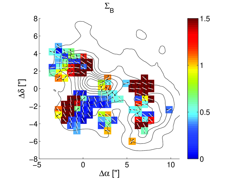
Figure 12.— Map of the local field significance. The dust continuum emission is shown in black contours. The color wedge indicates the force ratio, $\Sigma_{B}$, field tension force over gravitational pull. Values with $\Sigma_{B}<1$ indicate local gravitational collapse. White segements display the magnetic field orientations similar to the bottom panel in Figure 3. The dust emission gradient orientations are shown with black segments at the positions of polarized emission. The deviation between the two orientations is the angle $|\delta|\leq 90^{\circ}$, with a map-averaged $\langle|\delta|\rangle\approx 40^{\circ}$. A clear correlation in the two orientations is apparent with $\mathcal{C}=0.74$. Areas in blue translate into a mass-to-flux ratio of about 2-3 times the critical value.

5.5. Magnetic Field Flux Diffusion at Core Scales

The magnetic field strength in the DR 21(OH) core is only a factor two higher than the averaged value in the parsec scale filament, whereas the volume density is more than one order of magnitude higher. This suggests magnetic flux diffusion or dissipation. Assuming that the magnetic field strength has a power–law increase, i. e., $B\propto n({\rm H_{2}})^{\kappa}$, then we can use the densities and field strengths derived in the filament and in the core to derive the power–law index. From the values given in Table 4, $\kappa\ \simeq 0.2$. This is significantly lower than the value expected for a weak magnetic field with magnetic flux conservation, $\kappa=2/3$, (Crutcher et al., 1999). But it is also lower than the value predicted for the standard ambipolar diffusion models, $\kappa\simeq 0.44$–0.5, (Fiedler & Mouschovias, 1993). Ambipolar diffusion appears to be efficient only when densities reach values of $\gtrsim 10^{8}$  cm^-3 (Tassis & Mouschovias, 2007).

One possibility is that the diffusion arises from fast magnetic reconnection in the presence of turbulence (Lazarian & Vishniac, 1999; Santos-Lima et al., 2010). Recently, Leão et al. (2012) have carried out simulation to test this scenario in the case of gravitationally collapsing dense cores with initial turbulent to magnetic field energy ratios of 1.6–3. These values are clearly larger than the value found in the parsec scale filament, but are only slightly higher than the value found in the DR 21(OH) core. Leão et al. (2012) compute the temporal evolution of the average magnetic field–to–density ratio at the radius 0.3 pc in the core ($B_{0.3}/\rho_{0.3}$) normalized by the average value over the entire cloud, $(B/\rho$), which is 3.2 pc in their computation. We compute this value for the DR 21(OH) core, normalized by the average value in the filament. From Table 4, we obtain $(B_{\rm core}/\rho_{\rm core})/(B_{\rm filament}/\rho_{\rm filament})\simeq 0.042$. Note that the scales used here are different with respect to the ones used by Leão et al. (2012). The DR 21(OH) core has a radius of 0.04 pc, whereas the filament has an average radius of $\sqrt{4\times 0.34}=1.2$ pc (0.34 and 4 pc are roughly the length and thickness of the filament). Thus the scales and the scale ratio used in the DR 21(OH) region are different from the values used in the simulations. Nevertheless, the derived value can be used as a qualitative comparison between the simulations and our observations. Leão et al. (2012) find that in most cases, the aforementioned parameter is in the 0.1–0.3 range. Lower values are obtained only when Ohmic dissipation is included. Therefore, it is a feasible mechanism in the core.

5.6. Angular Momentum versus Magnetic Fields

The emission of the H¹³CO⁺ 4–3 line associated with the DR 21(OH) dense core shows a clear velocity pattern along the NE–SW direction (see Figures 7 and 8). This velocity gradient agrees with the one observed in the H¹³CO⁺ 1–0 and N₂H⁺ 1–0 line emission around the core (Schneider et al., 2010). These two lines trace well the large scale filament kinematics. These lines show an interesting E–W gradient with direction reversals along the filament. Schneider et al. (2010) interpret the velocity pattern in the filament as evidence of converging flows, which would have formed the filament. However, as already introduced in Section 3.4, the global kinematics in the core can be explained as Keplerian–like rotation. We speculate that the observed rotation has been induced by the large scale motions. The Keplerian–like rotation breaks in the inner region of the core, where the hottest and most massive condensations, SMA 6 and SMA 7, are located. Figure 8 shows that the Keplerian velocity distribution in the position–velocity cut along the major axis for a dynamical mass of $10\,{\rm M_{\odot}}/\cos(i)$ ($i$ is the inclination angle of the rotation axis in the plane of the sky) matches well the velocity pattern of the H¹³CO⁺ 4–3 emission. This mass is a lower limit, and, indeed, we can estimate how much mass is embedded in the inner part of DR 21(OH) assuming that the center of the core is dominated by SMA 6 and SMA 7. Zapata et al. (2012) estimates that the mass of these two hot cores is $\simeq 47$  $M_{\sun}$. If we consider the total luminosity of $\simeq 1\times 10^{4}$  $L_{\sun}$ in MM 1 to originate mainly from the two hot cores, then it is reasonable to assume that these two sources harbor protostars with a mass of at least $\simeq 13$  $M_{\sun}$. This yields a total mass of $\gtrsim 60$  $M_{\sun}$. This suggests a rotation axis of the core that is almost along the line-of-sight with $i\gtrsim 80\arcdeg$. Since a rotating envelope is expected to be somewhat flattened in the plane perpendicular to the rotation’s axis, this result suggests that DR 21(OH) is nearly face-on. This could explain the lack of flatness observed in the emission of both the dust continuum and of the H¹³CO⁺ 4–3 emission.

Machida et al. (2005) show that the importance of the angular momentum with respect to the magnetic fields can be measured from the ratio between the angular velocity and the magnetic field strength, $\omega/B$, with a critical value given by $(\omega/B)_{\rm crit}=3.19\times 10^{-8}\,c_{\rm s}^{-1}$ yr^-1 $\mu$G^-1, where $c_{\rm s}$ is the sound speed in  km s^-1. The sound speed for the temperature in the core, 30 K, is $c_{\rm s}=0.33$  km s^-1, so the critical value is $9.8\times 10^{-8}$ yr^-1 $\mu$G^-1. We can derive the angular velocity from Figure 8, adopting the core’s radius, $5\farcs 2$ (7800 AU). At this radius, the rotation velocity component along the line of sight is 1.1  km s^-1. Taking into account that the rotation axis has an inclination of $80\arcdeg$, the rotation velocity is $\simeq 6.3$  km s^-1. For the adopted radius, this yields an angular velocity of $\simeq 2\times 10^{-4}$ yr^-1 and an angular velocity-to-magnetic strength ratio of $\omega/B\simeq 8.4\times 10^{-8}$, which is similar to the critical value. This suggests that in DR 21(OH) the centrifugal energy is dynamically as important as the magnetic energy.

Going back to the magnetic field, to better understand its morphology, we have to take into account that we are looking at DR 21(OH) in a face-on projection. Theoretical models of rotating and magnetized envelopes show that, in a face-on configuration a spiral magnetic field pattern is expected if initially the rotation and magnetic field axes are aligned (e.g., Machida et al., 2005; Padovani et al., 2012; Kataoka et al., 2012). However, if this is not the case, a more complex morphology would be expected (Machida et al., 2005; Hennebelle & Ciardi, 2009). Therefore, the complex polarization pattern observed with the SMA in DR 21(OH) is probably due to the face-on orientation of magnetic field lines that are being wrapped and twisted by the core’s rotation. Indeed, we can estimate the angle of the average field with respect to the plane of the sky, $\alpha=\arctan(B_{\rm los}/B_{\rm pos})$. Using the values obtained from the CN Zeeman observations (Crutcher et al., 1999) and from the SMA dust polarization (see Section 4), the mean magnetic field has an inclination of only $\simeq 10\arcdeg$ with respect to the plane of the sky. This suggest that it has a toroidal configuration, which supports the evidence that the field lines are being dragged by the rotation. Simulations show that under these circumstances, the magnetic field tension would create a large-scale tower low-velocity outflow perpendicular to the flattened structure (Tomisaka, 1998; Peters et al., 2011). It is possible that the large-scale NW–SE, low-velocity CO outflow detected with the JCMT (Vallée & Fiege, 2006) is tracing this predicted tower flow. Note that this outflow is not detected with the SMA, suggesting that it has a wide origin.

A final issue about the angular momentum is that SMA 6 and SMA 7 appear to clearly depart from the Keplerian rotation, because from the hot-core lines the mean velocity is about 2 km s^-1 lower than the value expected for Keplerian rotation velocities (see the bottom panel of Figure 8). One possible explanation for this apparent lack of angular momentum conservation would be magnetic braking, which have already been observed in another massive dense core (Girart et al., 2009). However, an alternative possibility is that the angular momentum have been transferred into the formation of the two sub cores, SMA 6 and SMA 7.

5.7. The High Level of Fragmentation in DR 21(OH)

Recent simulations of massive dense molecular star-forming cores show that magnetic fields and radiative feedback can effectively suppress fragmentation (Tilley & Pudritz, 2007; Peters et al., 2011; Hennebelle et al., 2011; Myers et al., 2013), but that outflow feedback may promote fragmentation (Wang et al., 2010). Observationally, Palau et al. (2013) recently compiled a list of star forming regions that are in a very early phase, having luminosities between few hundreds and $\sim 10^{5}$  $L_{\sun}$, and having millimeter aperture synthesis observations with angular resolutions of $\lesssim 1000$ AU. They found a broad range of fragmentation, but with 30% showing no fragmentation in millimeter wavelengths. A comparison with simulations of turbulent and magnetized cores (Commerçon et al., 2011), suggests that the level of fragmentation can be related to the level of magnetization. Our SMA observation of DR 21(OH)  can be included in this list. By doing this, this source appears to be in the extreme case of fragmentation, with more than 10 millimeter sources detected. This is a case similar to OMC-1S-136 (Palau et al., 2013). The cases of high fragmentation can be explained if the cloud is only very weakly magnetized, with mass–to–flux ratios of $\sim 100$ (Commerçon et al., 2011; Myers et al., 2013). However, the dust continuum observations show that the mass–to–flux ratio is $\sim 6$. Even accounting for the mass already accreted onto the protostars in the DR 21(OH) core (possibly a factor less than two), the value is still much lower.

A high angular momentum of the core and the outflow feedback seem to be a plausible explanation for the DR 21(OH) fragmentation. First, following the Chen et al. (2012) recipe, we estimate the rotational energy-to-gravitational potential energy ratio for DR 21(OH) to be $\sim 0.5$ for the corrected projection of the rotation velocity. This value is an order of magnitude higher than the values reported in the Palau et al. (2013) survey, although the values derived in this survey were uncorrected for projection. However, since it is expected that this sample has a random distribution of source orientations, we can consider that DR 21(OH) is a core with a significantly higher value of angular momentum than the average core. Second, this source shows a very active outflow activity (see Section 3.5), with emission from high density tracers (Zapata et al., 2012) in the outflows and the presence of a rich variety of masers (see Section 1 for references).

6. Conclusions

We have carried out an extensive molecular, dust and polarimetric study of the massive DR 21(OH) star forming core from SMA high-angular-resolution observations at 880 $\mu$m. We have obtained observations from all the available SMA configurations (subcompact, compact, extended and very extended). We have also included complementary archival polarimetric observations from SCUPOL of the JCMT telescope (Matthews et al., 2009). All these data allow us to study and characterize the magnetic field properties from parsec scales down to 1000 AU toward a core that appears to be highly fragmented at smaller scales. The molecular line emission of selected transition detected with the SMA allows us to study the kinematic properties of the core and to put them into a context together with the magnetic field properties. Here, we summarize the main results:

1. The SMA maps at different angular resolutions ($3\farcs 6$-$0\farcs 75$) reveal a complex magnetic field morphology in the DR 21(OH) core. This is in contrast to the relatively smooth large-scale magnetic field threading the filamentary dense ridge where DR 21(OH) is embedded.

2. The $\sim 7.8$ GHz bandwidth reveals a rich molecular line spectra in the DR 21(OH) core. In particular, SMA 6 and SMA 7 have spectral features consistent with being hot molecular cores. The H¹³CO⁺ 4–3 emission correlates well with the dust emission at scales of 0.01–0.1 pc except toward the SMA 6 and SMA 7 hot cores. Therefore, this line is a good tracer of the overall DR 21(OH) core’s kinematics.

3. Combining the kinematic information from selected molecular tracers (H¹³CO⁺ 4–3 that traces the DR 21(OH) core except SMA 6 and SMA 7, ethyl cyanide tracing SMA 6, dimethyl ether tracing SMA 7), we find that the DR 21(OH) kinematics are compatible with Keplerian motions, except in the center of the core around SMA 6 and SMA 7. From the mass enclosed in SMA 6 and SMA 7, we estimate that the rotation axis is close to the line-of-sight. The DR 21(OH) core is, thus, probably observed face-on.

4. The HV CO 3–2 emission shows two collimated bipolar outflows approximately in the east-west direction, $PA\simeq 65\arcdeg$ and $110\arcdeg$. They are probably powered by SMA 7 and SMA 4, respectively. SMA 6 also powers a compact outflow in the N–S direction (Minh et al., 2011).

5. The statistical analysis reveals that the magnetic field is approximately in equipartition with the turbulent energy in the DR 21(OH) core, whereas in the filament the magnetic field energy dominates over turbulence. This possibly suggests that the star formation activity (for example through the powerful outflows) is injecting turbulence in the DR 21(OH) core. This analysis in DR 21(OH) yields a turbulent length scale, 16 mpc, and a magnetic field component in the plane of the sky, 2.1 mG. These values are in good agreement with the values derived from a completely independent method by Hezareh et al. (2010).

6. The total magnetic field strength derived, combining the dust measurements with previous Zeeman measurements (Crutcher, 2004), is 2.1 and 0.9 mG for the DR 21(OH) core and the parsec-scale filament, respectively. Both molecular structures are supercritical, in agreement with the observed large-scale infall motions (Schneider et al., 2010). The mass–to–flux ratios for the core and the ridge are 5.9 and 3.4 times the critical value, respectively. Thus, gravity has overcome the interstellar magnetohydrodynamic turbulence and the magnetic fields threading both the DR 21 filamentary ridge and especially the DR 21(OH) core. An independent analysis based on the polarization–intensity gradient method (Koch et al., 2012a) further confirms this finding with a map-averaged field-to-gravity force ratio of about 0.8, and some local areas where the field significance is reduced to $\sim$10% or less. The magnetic field direction has an inclination of only $\simeq 10\arcdeg$ with respect to the plane of the sky, suggesting a toroidal configuration.

7. In spite of being clearly supercritical, the high fragmentation observed in DR 21(OH) would require a much higher mass–to–flux ratio according to recent simulations of turbulent and magnetized clouds (Commerçon et al., 2011; Myers et al., 2013). It is possible that the high angular momentum measured is playing an important role in the fragmentation process of the DR 21(OH) core. First, the ratio between the angular velocity and the magnetic flux, $\omega/B$, is similar to the critical value, indicating that rotation is energetically as important as the magnetic fields in the dynamics of the core. This can explain the toroidal configuration of the magnetic field lines, as they are being wrapped by the rotation of the dense gas.

8. The wrapped and toroidal magnetic field configuration suggests that the previously reported large-scale low-velocity CO outflow (Vallée & Fiege, 2006), undetected with the SMA, is tracing the theoretically predicted large-scale tower flow (Peters et al., 2011).

References

- Alves et al. (2011) Alves, F. O., Girart, J. M., Lai, S.-P., Rao, R., & Zhang, Q. 2011, ApJ, 726, 63
- Araya et al. (2009) Araya, E. D., Kurtz, S., Hofner, P., & Linz, H. 2009, ApJ, 698, 1321
- Batrla & Menten (1988) Batrla, W., & Menten, K. M. 1988, ApJ, 329, L117
- Busquet et al. (2013) Busquet, G., Zhang, Q., Palau, A., et al. 2013, ApJ, 764, L26
- Chen et al. (2012) Chen, X., Arce, H. G., Dunham, M. M., & Zhang, Q. 2012, ApJ, 747, L43
- Commerçon et al. (2011) Commerçon, B., Hennebelle, P., & Henning, T. 2011, ApJ, 742, L9
- Cortes et al. (2005) Cortes, P. C., Crutcher, R. M., & Watson, W. D. 2005, ApJ, 628, 780
- Crutcher (2004) Crutcher, R. M. 2004, Ap&SS, 292, 225
- Crutcher (2012) Crutcher, R. M. 2012, ARA&A, 50, 29
- Crutcher et al. (1999) Crutcher, R. M., Troland, T. H., Lazareff, B., Paubert, G., & Kazès, I. 1999, ApJ, 514, L121
- Csengeri et al. (2011) Csengeri, T., Bontemps, S., Schneider, N., et al. 2011, ApJ, 740, L5
- Downes & Rinehart (1966) Downes, D., & Rinehart, R. 1966, ApJ, 144, 937
- Fiedler & Mouschovias (1993) Fiedler, R. A., & Mouschovias, T. C. 1993, ApJ, 415, 680
- Fish et al. (2011) Fish, V. L., Muehlbrad, T. C., Pratap, P., et al. 2011, ApJ, 729, 14
- Franco et al. (2010) Franco, G. A. P., Alves, F. O., & Girart, J. M. 2010, ApJ, 723, 146
- Frau et al. (2011) Frau, P., Galli, D., & Girart, J. M. 2011, A&A, 535, A44
- Frau et al. (2013) Frau, P., Girart, J. M., Zhang, Q., Rao, R., 2013, ApJ, in preparation
- Fromang et al. (2006) Fromang, S., Hennebelle, P., & Teyssier, R. 2006, A&A, 457, 371
- Galván-Madrid et al. (2010) Galván-Madrid, R., Zhang, Q., Keto, E., et al. 2010, ApJ, 725, 17
- Girart et al. (2009) Girart, J. M., Beltrán, M. T., Zhang, Q., Rao, R., & Estalella, R. 2009, Science, 324, 1408
- Girart et al. (1999) Girart, J. M., Crutcher, R. M., & Rao, R. 1999, ApJ, 525, L109
- Girart et al. (2006) Girart, J. M., Rao, R., & Marrone, D. P. 2006, Science, 313, 812
- Glenn et al. (1999) Glenn, J., Walker, C. K., & Young, E. T. 1999, ApJ, 511, 812
- Hakobian & Crutcher (2012) Hakobian, N. S., & Crutcher, R. M. 2012, ApJ, 758, L18
- Harvey et al. (1986) Harvey, P. M., Joy, M., Lester, D. F., & Wilking, B. A. 1986, ApJ, 300, 737
- Harvey-Smith et al. (2008) Harvey-Smith, L., Soria-Ruiz, R., Duarte-Cabral, A., & Cohen, R. J. 2008, MNRAS, 384, 719
- Hennebelle & Ciardi (2009) Hennebelle, P., & Ciardi, A. 2009, A&A, 506, L29
- Hennebelle et al. (2011) Hennebelle, P., Commerçon, B., Joos, M., et al. 2011, A&A, 528, A72
- Hennebelle & Fromang (2008) Hennebelle, P., & Fromang, S. 2008, A&A, 477, 9
- Hennemann et al. (2012) Hennemann, M., Motte, F., Schneider, N., et al. 2012, A&A, 543, L3
- Hezareh et al. (2010) Hezareh, T., Houde, M., McCoey, C., & Li, H.-b. 2010, ApJ, 720, 603
- Hildebrand et al. (2009) Hildebrand, R. H., Kirby, L., Dotson, J. L., Houde, M., & Vaillancourt, J. E. 2009, ApJ, 696, 567
- Ho et al. (2004) Ho, P. T. P., Moran, J. M., & Lo, K. Y. 2004, ApJ, 616, L1
- Houde et al. (2011) Houde, M., Rao, R., Vaillancourt, J. E., & Hildebrand, R. H. 2011, ApJ, 733, 109
- Houde et al. (2009) Houde, M., Vaillancourt, J. E., Hildebrand, R. H., Chitsazzadeh, S., & Kirby, L. 2009, ApJ, 706, 1504
- Hull et al. (2013) Hull, C. L. H., Plambeck, R. L., Bolatto, A. D., et al. 2013, ApJ, 768, 159
- Jakob et al. (2007) Jakob, H., Kramer, C., Simon, R., et al. 2007, A&A, 461, 999
- Jewell et al. (1989) Jewell, P. R., Hollis, J. M., Lovas, F. J., & Snyder, L. E. 1989, ApJS, 70, 833
- Kataoka et al. (2012) Kataoka, A., Machida, M. N., & Tomisaka, K. 2012, ApJ, 761, 40
- Keto & Zhang (2010) Keto, E., & Zhang, Q. 2010, MNRAS, 406, 102
- Kirby (2009) Kirby, L. 2009, ApJ, 694, 1056
- Koch et al. (2010) Koch, P. M., Tang, Y.-W., & Ho, P. T. P. 2010, ApJ, 721, 815
- Koch et al. (2012a) Koch, P.M., Tang, Y.-W., & Ho, P.T.P. 2012a, ApJ, 747, 79
- Koch et al. (2012b) Koch, P.M., Tang, Y.-W., & Ho, P.T.P. 2012b, ApJ, 747, 80
- Kurtz et al. (2004) Kurtz, S., Hofner, P., & Álvarez, C. V. 2004, ApJS, 155, 149
- Lai et al. (2002) Lai, S.-P., Crutcher, R. M., Girart, J. M., & Rao, R. 2002, ApJ, 566, 925
- Lai et al. (2003) Lai, S.-P., Girart, J. M., & Crutcher, R. M. 2003, ApJ, 598, 392
- Larson (1981) Larson, R. B. 1981, MNRAS, 194, 809
- Lazarian & Vishniac (1999) Lazarian, A., & Vishniac, E. T. 1999, ApJ, 517, 700
- Leão et al. (2012) Leão, M. R. M., de Gouveia Dal Pino, E. M., Santos-Lima, R., & Lazarian, A. 2012, arXiv:1209.1846
- Machida et al. (2005) Machida, M. N., Matsumoto, T., Tomisaka, K., & Hanawa, T. 2005, MNRAS, 362, 369
- Mayer et al. (1973) Mayer, C. H., Waak, J. A., Cheung, A. C., & Chui, M. F. 1973, ApJ, 182, L65
- Marrone et al. (2006) Marrone, D. P., Moran, J. M., Zhao, J.-H., & Rao, R. 2006, ApJ, 640, 308
- Marrone & Rao (2008) Marrone, D. P., & Rao, R. 2008, Proc. SPIE, 7020
- Matthews et al. (1986) Matthews, H. E., Baudry, A., Guilloteau, S., & Winnberg, A. 1986, A&A, 163, 177
- Matthews et al. (2009) Matthews, B.C., McPhee, C., Fissel, L., & Curran, R.L. 2009, ApJS, 182, 143
- Minchin & Murray (1994) Minchin, N. R., & Murray, A. G. 1994, A&A, 286, 579
- Minh et al. (2011) Minh, Y. C., Liu, S.-Y., Chen, H.-R., & Su, Y.-N. 2011, ApJ, 737, L25
- Mookerjea et al. (2012) Mookerjea, B., Hassel, G. E., Gerin, M., et al. 2012, A&A, 546, A75
- Motte et al. (2007) Motte, F., Bontemps, S., Schilke, P., et al. 2007, A&A, 476, 1243
- Myers et al. (2013) Myers, A. T., McKee, C. F., Cunningham, A. J., Klein, R. I., & Krumholz, M. R. 2013, ApJ, 766, 97
- Ossenkopf & Henning (1994) Ossenkopf, V., & Henning, T. 1994, A&A, 291, 943
- Padovani et al. (2012) Padovani, M., Brinch, C., Girart, J. M., et al. 2012, A&A, 543, A16
- Palau et al. (2013) Palau, A., Fuente, A., Girart, J. M., et al. 2013, ApJ, 762, 120
- Peters et al. (2011) Peters, T., Banerjee, R., Klessen, R. S., & Mac Low, M.-M. 2011, ApJ, 729, 72
- Plambeck & Menten (1990) Plambeck, R. L., & Menten, K. M. 1990, ApJ, 364, 555
- Poidevin et al. (2010) Poidevin, F., Bastien, P., & Matthews, B. C. 2010, ApJ, 716, 893
- Rao et al. (2009) Rao, R., Girart, J. M., Marrone, D. P., Lai, S.-P., & Schnee, S. 2009, ApJ, 707, 921
- Reipurth & Schneider (2008) Reipurth, B., & Schneider, N. 2008, Handbook of Star Forming Regions, Volume I, 36
- Rygl et al. (2012) Rygl, K. L. J., Brunthaler, A., Sanna, A., et al. 2012, A&A, 539, A79
- Santos-Lima et al. (2010) Santos-Lima, R., Lazarian, A., de Gouveia Dal Pino, E. M., & Cho, J. 2010, ApJ, 714, 442
- Schneider et al. (2010) Schneider, N., Csengeri, T., Bontemps, S., et al. 2010, A&A, 520, A49
- Seifried et al. (2012) Seifried, D., Banerjee, R., Pudritz, R. E., & Klessen, R. S. 2012, MNRAS, 423, L40
- Tang et al. (2009a) Tang, Y.-W., Ho, P. T. P., Girart, J. M., et al. 2009a, ApJ, 695, 1399
- Tang et al. (2009b) Tang, Y.-W., Ho, P. T. P., Koch, P. M., et al. 2009b, ApJ, 700, 251
- Tang et al. (2010) Tang, Y.-W., Ho, P. T. P., Koch, P. M., & Rao, R. 2010, ApJ, 717, 1262
- Tang et al. (2013) Tang, Y.-W., Ho, P. T. P., Koch, P. M., Guilloteau, S., & Dutrey, A. 2013, ApJ, 763, 135
- Tassis & Mouschovias (2007) Tassis, K., & Mouschovias, T. C. 2007, ApJ, 660, 388
- Tilley & Pudritz (2007) Tilley, D. A., & Pudritz, R. E. 2007, MNRAS, 382, 73
- Tomisaka (1998) Tomisaka, K. 1998, ApJ, 502, L163
- Turner (1992) Turner, B. E. 1992, ApJ, 396, L107
- Vallée & Fiege (2006) Vallée, J. P., & Fiege, J. D. 2006, ApJ, 636, 332
- Wang et al. (2010) Wang, P., Li, Z.-Y., Abel, T., & Nakamura, F. 2010, ApJ, 709, 27
- Woody et al. (1989) Woody, D. P., Scott, S. L., Scoville, N. Z., et al. 1989, ApJ, 337, L41
- Zapata et al. (2012) Zapata, L. A., Loinard, L., Su, Y.-N., et al. 2012, ApJ, 744, 86
- Zhang et al. (2002) Zhang, Q., Hunter, T. R., Sridharan, T. K., & Ho, P. T. P. 2002, ApJ, 566, 982