Hydrodynamic theory of coupled current and magnetization dynamics in spin-textured antiferromagnets

Abstract

Antiferromagnets with vanishingly small (or zero) magnetization are interesting candidates for spintronics applications. In the present paper we propose two models for description of the current-induced phenomena in antiferromagnetic textures. We show that the magnetization that originates from rotation or oscillations of antiferromagnetic vector can, via $sd$-exchange coupling, polarize the current and give rise to adiabatic and nonadiabatic spin torques. Due to the Lorentz-type dynamics of antiferromagnetic moments (unlike the Galilenian-like dynamics in ferromagnets), the adiabatic spin torque affects the characteristic lengthscale of the moving texture. Nonadiabatic spin torque contributes to the energy pumping and can induce the stable motion of antiferromagnetic texture, but, in contrast to ferromagnets, has pure dynamic origin. We also consider the current-induced phenomena in artificial antiferromagnets where the current maps the staggered magnetization of the structure. In this case the effect of nonadiabatic spin torque is similar to that in ferromagnetic constituents of the structure. In particular, the current can remove degeneracy of the translational antiferromagnetic domains indistinguishable in the external magnetic field and thus can set into motion the 180^∘ domain wall.

I Introduction

Spin-polarized current flowing through the magnetic layers gives rise to variety of different phenomena with interesting physics and wide range of applications. In particular, the current can transfer a torque and thus produce a spin-motive force for the system of localized magnetic moments. This effect is responsible for rotation of ferromagnetic magnetization in discrete systems or movement of domain wall in continuous textures.

Spin-torque phenomena, as predicted by Slonczewski Slonczewski:1996 and Berger Berger:1996 , originate from the spin-conserving exchange interactions between itinerant and localized electrons (so-called $sd$-exchange) and are usually modeled with the Heisenberg-type Hamiltonian

$$\hat{\mathcal{H}}_{\mathrm{sd}}=-\sum_{\mathbf{R}_{\mathbf{n}}}J_{\mathrm{sd}}(\mathbf{r}-\mathbf{R}_{\mathbf{n}})\hat{\mathbf{s}}(\mathbf{r})\hat{\mathbf{S}}(\mathbf{R}_{\mathbf{n}})$$ (1)

where $J_{\mathrm{sd}}$ is the exchange integral, $\hat{\mathbf{s}}(\mathbf{r})$ and $\hat{\mathbf{S}}(\mathbf{R}_{\mathbf{n}})$ are spin operators of free ($s$) and localized ($d$) at a site $\mathbf{R}_{\mathbf{n}}$ electrons, respectively.

In the semiclassical approach Zhang:PhysRevLett.93.127204 that assumes rather slow dynamics of localized spins compared to the itinerant ones, the system of localized magnetic moments is treated classically. Particularly, in ferromagnets (FMs) the spin operators $\hat{\mathbf{S}}(\mathbf{R}_{\mathbf{n}})$ are replaced with the magnetization vector $\mathbf{M}(\mathbf{r},t)$, and the averaged over all electronic states spin $\hat{\mathbf{s}}$ is replaced with the normalized electron magnetization density $\mathbf{m}$ ($|\mathbf{m}|=1$). Thus, the energy density of $sd$-exchange, derived from Hamiltonian (1), takes a form

$$\mathcal{H}_{\mathrm{sd}}(\mathbf{r})=-\frac{J_{\mathrm{sd}}}{M_{s}}\mathbf{m}\cdot\mathbf{M},$$ (2)

where $M_{s}$ is saturation magnetization.

Interactions described by Eqs. (1) and (2) determine the processes of current polarization and transfer of spin torque. In FMs with the pronounced value of equilibrium magnetization $\mathbf{M}$ the effects related with $sd$-interaction are quite strong.

However, application of the same ideas to other magnetic materials, – antiferromagnets (AFMs), with zero or vanishingly small equilibrium magnetization, – poses new challenges as compared to FMs. Macroscopic magnetization $\mathbf{M}_{\mathrm{AFM}}$ in AFMs has mainly dynamic origin. Its value is weakened (compared to FMs) by relatively small magnetic susceptibility. On the other hand, AFM ordering is characterized with macroscopic vector(s) $\mathbf{L}_{k}$ ($k=1,2\ldots N_{\mathrm{sub}}$, where $N_{\mathrm{sub}}$ depends upon the number of magnetic sublattices) which reproduce a space distribution of staggered magnetization and in most cases belong to another than $\mathbf{M}_{\mathrm{AFM}}$ irreducible representation of the space group (i.e., have different symmetry properties). In this case the semiclassical expression for the density of $sd$-exchange, as follows from general symmetry considerations, takes a form (cp. with (2)):

$$\mathcal{H}_{\mathrm{sd}}(\mathbf{r})=-\frac{1}{{M_{s}}}\left[J^{\mathrm{FM}}_{\mathrm{sd}}\mathbf{m}\cdot\mathbf{M}_{\mathrm{AFM}}+J^{\mathrm{AFM}}_{\mathrm{sd}}\sum_{k=1}^{N_{\mathrm{sub}}}\mathbf{l}_{k}\cdot\mathbf{L}_{k}\right],$$ (3)

where vectors $\mathbf{l}_{k}$, which characterize the itinerant electrons, should belong to the same irreducible representation as $\mathbf{L}_{k}$ and $J^{\mathrm{FM}}_{\mathrm{sd}}$, $J^{\mathrm{AFM}}_{\mathrm{sd}}$ are the corresponding exchange constants.

The first, “standard”, or FM-like, term in the Eq. (3) may induce rotation of AFM moments once the current is already polarized by the external FM layer Haney:2007(2) ; Tsoi:2007 ; gomo:2010 ; Gomonay:PhysRevB.85.134446 . The second, “specific”, or AFM-like term, if any, may induce a special – AFM – polarization of current and thus should be important in AFM textures (see, e.g., Ref. Nunez:2005 ). Whether both terms exist and how important they are significantly depends upon topology of the Fermi surface and density of states.

In the present paper we address two mutually related questions: i) what current-induced effects could be anticipated in AFM textures from the first ($J^{\mathrm{FM}}_{\mathrm{sd}}\neq 0,J^{\mathrm{AFM}}_{\mathrm{sd}}=0$) and the second ( $J^{\mathrm{AFM}}_{\mathrm{sd}}\neq 0$) constituents of $sd$-exchange; and ii) in what cases spin density of the itinerant (represented by AFM vectors $\mathbf{l}_{k}$) electrons may have space modulation that identically maps the space distribution of localized moments imposed by crystal lattice. Starting from hydrodynamic approach for microscopic dynamics of AFMs Andreev:1980 we derive the close set of equations for AFM vectors in the presence of current assuming the FM-like ($J^{\mathrm{AFM}}_{\mathrm{sd}}=0$) form of $sd$-exchange. We show existence of adiabatic and nonadiabatic spin torques (AST and NAST, respectively) and demonstrate their dynamic origin. NAST, though small compared with AST (and NAST in ferromagnetic textures) can compensate the internal losses in the moving domain walls.

To illustrate the role of the second, AFM-like contribution to $sd$-exchange, we consider the current-induced dynamics in artificial AFMs. AST and NAST in this case have the same values and reveal themselves in a similar way as in FMs. In particular, the current (in contrast to constant magnetic field ) can set into motion the 180^∘ AFM domain wall (DW) that separates translational domains.

II Effect of ferromagnetic-like $sd$-exchange: antiferromagnetic texture

Let us consider an AFM conductor with well separated systems of localized and free (conduction) electrons. Good example of such materials is given by AFM metals FeMn and IrMn, or by metallic antiperovskites Mn₃MN (where M=Ag, Ni). Following the phenomenological approaches deduced for FM textures (see, e.g. Refs. Zhang:PhysRevLett.93.127204 ; Sun:2011EPJB_79_449S ) we describe the average magnetization of free electrons with the field variable $\mathbf{m}(\mathbf{r},t)$ and assume $sd$-exchange interaction in a form (3) with $J^{\mathrm{AFM}}_{\mathrm{sd}}=0$.

Description of localized moments needs some special comments. In spite of diversity of possible magnetic structures, the low-frequency dynamics of AFMs can be expressed in terms of at most three independent variables that represent a so-called “solid-like” rotation of localized magnetic moments Andreev:1980 . In this section we consider the case of multisublattice AFM with isotropic magnetic susceptibility $\chi$ and parametrize spin rotations with the Gibbs’ vector $\boldsymbol{\varphi}=\varphi\mathbf{e}$, where the unit vector $\mathbf{e}$ defines an instantaneous rotation axis, $\varphi=\tan(\theta/2)$, and $\theta$ is the rotation angle (for the details see the papers Refs. Andreev:1980 ; Gomonay:PhysRevB.85.134446 ). While the components of Gibbs’ vector $\boldsymbol{\varphi}$ form a set of coordinates, the components of spin rotation frequency, expressed as follows:

$$\mathbf{\Omega}=2\frac{\dot{\boldsymbol{\varphi}}+\boldsymbol{\varphi}\times\dot{\boldsymbol{\varphi}}}{1+{\boldsymbol{\varphi}^{2}}},$$ (4)

are conjugated generalized velocities. Here the sign “$\times$” means cross-product.

Then, macroscopic magnetization of AFM is proportional to spin rotation frequency, $\mathbf{\Omega}$, and external magnetic field $\mathbf{H}$:

$$\mathbf{M}_{\mathrm{AFM}}=\frac{\chi}{\gamma}\left(\boldsymbol{\Omega}+\gamma\mathbf{H}\right),$$ (5)

where $\gamma$ is gyromagnetic ratio.

The dynamic equations for localized AFM moments are deduced from the spin conservation principle which takes a form of the balance equation:

$$\frac{d\mathbf{M}_{\mathrm{AFM}}}{dt}=\nabla\cdot\hat{\boldsymbol{\Pi}},\quad\textrm{or}\quad\frac{dM_{\mathrm{AFM}}^{(\alpha)}}{dt}=\frac{\partial\Pi_{\alpha\beta}}{\partial x_{\beta}},$$ (6)

where $\hat{\boldsymbol{\Pi}}$ is the 2-nd rank tensor of the magnetization flux density induced, in particular, by spin-polarized current. With account of the relation (5) the dynamic Eq. (6) for the localized AFM moments in the most general case can be written as follows:

$$\frac{2\chi}{\gamma^{2}}\lambda_{\beta\alpha}\frac{d}{dt}\left[\left(\Omega_{\beta}+\gamma H_{\beta}\right)\right]+\frac{2\chi}{\gamma}\lambda_{\beta\alpha}(\mathbf{H}\times\boldsymbol{\Omega})_{\beta}+\frac{\partial U_{\mathrm{AFM}}}{\partial\varphi_{\alpha}}=\frac{2}{\gamma}\lambda_{\beta\alpha}\nabla_{\delta}\Pi_{\beta\delta},$$ (7)

where the potential $U_{\mathrm{AFM}}(\boldsymbol{\varphi})$ describes the magnetic anisotropy of AFM and includes gradient terms of the exchange nature, tensor $\lambda_{\alpha\beta}$ defines the metrics in $\boldsymbol{\varphi}$ space:

$$\lambda_{\alpha\beta}=\frac{\delta_{\alpha\beta}+\varepsilon_{\alpha\gamma\beta}\varphi_{\gamma}}{1+{\boldsymbol{\varphi}^{2}}},$$ (8)

and $\varepsilon_{\alpha\gamma\beta}$ is the (completely antisymmetric) Levi-Civita symbol.

Analysis of the Eq. (5) shows that AFMs with an arbitrary magnetic structure have nonzero magnetization $\mathbf{M}_{\mathrm{AFM}}$ even in the absence (or neglection) of the external Oersted magnetic field, though this magnetization has pure dynamic origin ($\mathbf{M}_{\mathrm{AFM}}\propto\boldsymbol{\Omega})$. So, AFM can polarize the conduction electrons through the $sd$-exchange interactions (3) even if $J^{\mathrm{AFM}}_{\mathrm{sd}}=0$.

To obtain equations for normalized magnetization of free electrons, $\mathbf{m}(\mathbf{r},t)$, we represent it as a sum of equilibrium, $\mathbf{m}_{\mathrm{eq}}$, and small nonequilibrium, $\delta\mathbf{m}(\mathbf{r},t)$, contributions:

$$\mathbf{m}(\mathbf{r},t)=\mathbf{m}_{\mathrm{eq}}(\mathbf{r})+\delta\mathbf{m}(\mathbf{r},t).$$ (9)

If time variation of localized moments is slow compared with the carrier’s spin-flip relaxation, then, equilibrium magnetization of conduction electrons maps distribution of AFM magnetization $\mathbf{M}_{\mathrm{AFM}}$. Thus, in analogy with FM,

$$\mathbf{m}_{\mathrm{eq}}(\mathbf{r})=n_{\mathrm{eq}}\frac{\mathbf{M}_{\mathrm{AFM}}}{M_{s}}=\frac{\chi}{\gamma}\frac{n_{\mathrm{eq}}}{M_{s}}\boldsymbol{\Omega},$$ (10)

where $n_{\mathrm{eq}}$ is the local equilibrium density of carriers whose spin is parallel to $\mathbf{M}_{\mathrm{AFM}}$.

On the other hand, nonequilibrium magnetization $\delta\mathbf{m}$ is created in the AFM texture due to time and spatial variation of $\mathbf{M}_{\mathrm{AFM}}$. For the case of slow space variations (i.e. the spin-diffusion length is much smaller than the typical DW width) the dynamic equation for $\delta\mathbf{m}$ takes a form similar to that in FMs Zhang:PhysRevLett.93.127204 :

$$-\frac{\delta\mathbf{m}}{\tau_{\mathrm{sf}}}-\frac{J_{\mathrm{sd}}}{\hbar M_{s}}\delta\mathbf{m}\times\mathbf{M}_{\mathrm{AFM}}=\frac{n_{\mathrm{eq}}}{M_{s}}\frac{\partial\mathbf{M}_{\mathrm{AFM}}}{\partial t}-\frac{P}{eM_{s}}(\mathbf{j}\cdot\nabla)\mathbf{M}_{\mathrm{AFM}}$$ (11)

where $\tau_{\mathrm{sf}}$ is the time of spin-flip relaxation, $P$ is the spin polarization factor, $e$ is electron charge, $\mathbf{j}$ is the electric current density.

The left-hand side of Eq. (11) includes two terms: the first one corresponds to spin relaxation of free electrons with the characteristic time $\tau_{\mathrm{sf}}$, and the second one describes rotation of free electron magnetization around localized magnetization $\mathbf{M}_{\mathrm{AFM}}$. In FMs, where $|\mathbf{M}_{\mathrm{FM}}|=M_{s}$, the second term is much greater than the first one, corresponding relation $\tau_{\mathrm{sf}}J_{\mathrm{sd}}/\hbar\propto 10\div 10^{2}$ is based on the typical values for FM metals like Fe, Ni and Co: $\tau_{\mathrm{sf}}\propto 10^{-12}$ s, $J_{\mathrm{sd}}\propto 1$ eV Zhang:PhysRevLett.93.127204 . In contrast, in AFM materials the relation between these two terms is reversed. Taking for estimation $\Omega$ of the order of AFMR frequency $\Omega_{\mathrm{AFMR}}\propto\gamma M_{s}\sqrt{H_{\mathrm{an}}H_{\mathrm{ex}}}$ (where $H_{\mathrm{an}}$ and $H_{\mathrm{ex}}=M_{s}/\chi$ are the anisotropy and exchange fields for localized moments) we get from (5) for the typical AFMs (FeMn, IrMn, NiO) $|\mathbf{M}_{\mathrm{AFM}}|/M_{s}\propto\sqrt{H_{\mathrm{an}}/H_{\mathrm{ex}}}\propto 1\div 3\cdot 10^{-2}$. Typical value of $J_{\mathrm{sd}}\propto 0.1\div 0.01$ eV Vonsovskii , so, for the same value of spin-flip relaxation, $\tau_{\mathrm{sf}}J_{\mathrm{sd}}|\mathbf{M}_{\mathrm{AFM}}|/(\hbar M_{s})\propto 10^{-2}\ll 1$.

With account of the above relation, the Eq. (11) can be solved in terms of rotation frequency as follows:

$$\delta\mathbf{m}=\frac{\chi\tau_{\mathrm{sf}}}{\gamma M_{s}}\left[-n_{\mathrm{eq}}\dot{\boldsymbol{\Omega}}+\frac{P}{e}(\mathbf{j}\cdot\nabla)\boldsymbol{\Omega}\right].$$ (12)

Magnetization of current enters dynamic Eqs. (7) for AFM vectors in two ways. First, equilibrium magnetization (10) of free electrons produces the magnetization flux

$$\boldsymbol{\Pi}=\frac{\chi\mu_{B}P}{\gamma eM_{s}}\mathbf{j}\otimes\boldsymbol{\Omega}=\frac{\chi}{\gamma}b_{\mathrm{AFM}}\mathbf{j}\otimes\boldsymbol{\Omega},\quad b_{\mathrm{AFM}}\equiv\frac{\mu_{B}P}{eM_{s}},$$ (13)

that should be substituted into r.h.s. of Eq. (7), and $\mu_{B}$ is the Bohr magneton.

Second, nonequilibrium magnetization, due to $sd$-interactions, produces in AFM an additional magnetic field

$$\gamma\mathbf{H}_{\mathrm{add}}\equiv-\gamma\frac{\partial\mathcal{H}_{\mathrm{sd}}}{\partial\mathbf{M}_{\mathrm{AFM}}}=\gamma\frac{J^{\mathrm{FM}}_{\mathrm{sd}}}{M_{s}}\delta\mathbf{m}=-\chi\epsilon_{\mathrm{AFM}}\dot{\boldsymbol{\Omega}}+c_{\mathrm{AFM}}(\mathbf{j}\cdot\nabla)\boldsymbol{\Omega},$$ (14)

where we introduced the phenomenological constants

$$\epsilon_{\mathrm{AFM}}\equiv\frac{\tau_{\mathrm{sf}}J^{\mathrm{FM}}_{\mathrm{sd}}}{M^{2}_{s}}n_{\mathrm{eq}},\qquad c_{\mathrm{AFM}}\equiv\frac{\chi\tau_{\mathrm{sf}}}{eM^{2}_{s}}J^{\mathrm{FM}}_{\mathrm{sd}}P=b_{\mathrm{AFM}}\frac{\tau_{\mathrm{sf}}J^{\mathrm{FM}}_{\mathrm{sd}}}{\mu_{B}H_{\mathrm{ex}}},$$ (15)

and $H_{\mathrm{ex}}=M_{s}/\chi$, as above.

Additional, current-induced field (14) plays a role of the external dissipation force that results, as will be shown below, in variation (relaxation or pumping) of the magnetic energy of localized moments.

Substituting (13) and (14) into (7) one gets equation for AFM texture in the presence of spin-polarized dc current:

$$\dot{\boldsymbol{\Omega}} + 2\gamma_{\mathrm{AFM}}\boldsymbol{\Omega}-\underbrace{\chi\epsilon_{\mathrm{AFM}}\left[\ddot{\boldsymbol{\Omega}}+\dot{\boldsymbol{\Omega}}\times\boldsymbol{\Omega}\right]}_{\mathrm{damping}}+\frac{\gamma^{2}}{2\chi}\hat{\lambda}^{-1}\frac{\partial U_{\mathrm{AFM}}}{\partial\boldsymbol{\varphi}}=$$ (16)

$$= \underbrace{b_{\mathrm{AFM}}(\mathbf{j}\cdot\nabla)\boldsymbol{\Omega}}_{\mathrm{AST}}-\underbrace{c_{\mathrm{AFM}}\left[(\mathbf{j}\cdot\nabla)\dot{\boldsymbol{\Omega}}-\boldsymbol{\Omega}\times(\mathbf{j}\cdot\nabla)\boldsymbol{\Omega}\right]}_{\mathrm{NAST}},$$

where we introduced the internal damping with factor $2\gamma_{\mathrm{AFM}}$ calculated as a linewidth of AFMR, $\hat{\lambda}^{-1}$ is the tensor inverse to $\hat{\lambda}$. Mind, that the damping coefficient $\gamma_{\mathrm{AFM}}$ differs from the analogous coefficient for FM system due to so-called exchange enhancement: $\gamma_{\mathrm{AFM}}\propto\gamma_{\mathrm{FM}}/\chi$, see, e.g., Ref. gomo:2010 .

Equation (16) includes three groups of terms that stipulate from interaction between localized and free electrons. The first group, with factor $\epsilon_{\mathrm{AFM}}$, is independent on current. It accounts for additional damping related with the itinerant electrons. To clarify this moment let us consider the simple example of AFM rotation (or oscillation) around a fixed axis $\mathbf{e}$. In this case $\boldsymbol{\Omega}=\dot{\theta}\mathbf{e}$. In the absence of current ($\mathbf{j}=0$) Eq. (16) takes a form:

$$\ddot{\theta}+2\gamma_{\mathrm{AFM}}\dot{\theta}-\chi\epsilon_{\mathrm{AFM}}\dddot{\theta}+\frac{\gamma^{2}}{\chi}\frac{\partial U_{\mathrm{AFM}}}{\partial\theta}=0.$$ (17)

For small oscillations with frequency $\Omega_{\mathrm{AFMR}}$ the effective damping is renormalized as follows:

$$2\gamma_{\mathrm{AFM}}\quad\Rightarrow\quad 2\gamma_{\mathrm{AFM}}+\chi\epsilon_{\mathrm{AFM}}\Omega^{2}_{\mathrm{AFMR}}.$$ (18)

Analogous effect is observed in FMs, however, renormalization (18) in AFMs is frequency-dependent. It should be mentioned that combination $\chi\Omega^{2}_{\mathrm{AFMR}}$ in AFMs is proportional to the magnetic anisotropy which is usually small. In general case the additional damping results from rotation around fixed axis (term $\ddot{\boldsymbol{\Omega}}$) and from the axis rotation (term $\dot{\boldsymbol{\Omega}}\times\boldsymbol{\Omega}$). However, these contributions are important for fast modes only and could be neglected for $\Omega\leq\Omega_{\mathrm{AFMR}}$.

It worth to note that the above introduced damping ($\propto\gamma_{\mathrm{AFM}}\boldsymbol{\Omega}$) models the “viscous resistance” against the solid-like motion of localized magnetic moments. In other words, we neglect the “exchange damping” that hampers mutual rotation of the magnetic sublattices and growth of $\mathbf{M}_{\mathrm{AFM}}$. The rather complicated problems of the exchange damping are out of scope of this paper, however, within the simplest phenomenological model (see, e.g.Bar'yakhtar:1984E ; Tserkovnyak:PhysRevLett.106.107206 ) corresponding contribution into equation of motion is proportional to high order time/space derivatives and thus has the same structure as $\epsilon_{\mathrm{AFM}}$-term in (16).

The second group, with the factor $b_{\mathrm{AFM}}$, is analogous to (and its value coincides with) the AST in FMs Bazaliy:PhysRevB.57.R3213 ; Zhang:PhysRevLett.93.127204 . The value $b_{\mathrm{AFM}}\mathbf{j}$, which, in fact, is independent on $sd$-exchange constant, can be interpreted as a relative velocity of AFM texture with respect to steady current. So, AST produces a similar kinematic effect in FM and AFM textures. However, in contrast to FMs, this term cannot be excluded from Eqs. (16). To illustrate this fact, we again consider rotation of AFM vectors around the fixed axis $\mathbf{e}$ and take into account inhomogeneous exchange coupling (constant $\alpha_{\mathrm{inh}}$) and possible nonlinearity of the magnetic anisotropy (modeled with the potential $U_{\mathrm{an}}(\theta)$):

$$U_{\mathrm{AFM}}=\frac{1}{2}\alpha_{\mathrm{inh}}\left(\nabla\theta\right)^{2}+U_{\mathrm{an}}(\theta).$$ (19)

Then, in neglection of dissipation (that includes damping and NAST) Eq. (17) takes a form:

$$\ddot{\theta}-{v_{\mathrm{mag}}^{2}}\Delta\theta+\frac{\gamma^{2}}{\chi}\frac{dU_{\mathrm{an}}}{d\theta}=b_{\mathrm{AFM}}(\mathbf{j}\cdot\nabla)\dot{\theta},$$ (20)

where $v_{\mathrm{mag}}\equiv\gamma\sqrt{\alpha_{\mathrm{inh}}/\chi}$ is the minimal phase velocity of magnons Ivanov:1983E . In the absence of current and anisotropy, Eq. (20) describes the Lorentz-invariant dynamics (as was noticed for the first time in Ref. Bar_jun:1983 for the collinear AFM). As a result, AST redefines the characteristic lengthscale of stationary moving nonlinear waves. Really, the solution of Eq. (20), $\theta_{\mathrm{stab}}(x-v_{\mathrm{DW}}t)$, that describes a solitary wave moving with the constant velocity $v_{\mathrm{DW}}$ along the current direction ($\mathbf{j}\|x$), should satisfy the following equation

$$\left(v_{\mathrm{mag}}^{2}-b_{\mathrm{AFM}}jv_{\mathrm{DW}}-{v_{\mathrm{DW}}^{2}}\right)\frac{d^{2}\theta}{dx^{2}}=\frac{\gamma^{2}}{\chi}\frac{dU_{\mathrm{an}}}{d\theta}.$$ (21)

Thus, the characteristic scale of inhomogeneity, $x_{\mathrm{DW}}$, is current-dependent:

$$x_{\mathrm{DW}}\quad\Rightarrow\quad\frac{x_{\mathrm{DW}}}{\sqrt{1-b_{\mathrm{AFM}}jv_{\mathrm{DW}}/v_{\mathrm{mag}}-{v_{\mathrm{DW}}^{2}/v_{\mathrm{mag}}^{2}}}}.$$ (22)

At last, the third group in Eq. (16) is responsible for NAST which can compensate the internal losses and provide, in combination with the external magnetic field, a stable motion of the AFM DW. For illustration we rewrite Eq. (21) for one dimensional inhomogeneuity in the current direction ($\mathbf{j}\|x$) with account of dissipation, NAST, and the constant external magnetic field $H$ that sets the DW into motion:

$$\ddot{\theta}-b_{\mathrm{AFM}}j\frac{\partial\dot{\theta}}{\partial x}-{v_{\mathrm{mag}}^{2}}\frac{\partial^{2}\theta}{\partial x^{2}}+\frac{\gamma^{2}}{\chi}\frac{dU_{\mathrm{an}}}{d\theta}=-2\gamma_{\mathrm{AFM}}\dot{\theta}+c_{\mathrm{AFM}}j\frac{\partial\ddot{\theta}}{\partial x}+\frac{\gamma^{2}}{2}H^{2}\sin 2\theta.$$ (23)

Equation (23) can be treated as the Lagrange equation in the presence of the external dissipative forces with the Lagrange function

$$\mathcal{L}=\frac{\chi}{2\gamma^{2}}\left(\dot{\theta}-b_{\mathrm{AFM}}j\frac{\partial\theta}{\partial x}\right)^{2}-\frac{\chi}{2\gamma^{2}}\left(v_{\mathrm{mag}}^{2}-b^{2}_{\mathrm{AF}}j^{2}\right)\left(\frac{\partial\theta}{\partial x}\right)^{2}-U_{\mathrm{an}}(\theta)-\frac{\chi H^{2}}{4}\sin^{2}\theta$$ (24)

and dissipation Rayleigh function

$$\mathcal{R}=\frac{\chi}{\gamma^{2}}\left(\gamma_{\mathrm{AFM}}\dot{\theta}^{2}-c_{\mathrm{AFM}}j\dot{\theta}\frac{\partial^{2}}{\partial t^{2}}\frac{\partial{\theta}}{\partial x}\right),$$ (25)

where generalized thermodynamic forces $\partial\theta/\partial x$ are fixed (i.e. variation of the Rayleigh function should be taken with respect to generalized velocities $\dot{\theta}$ only).

In the absence of current Eq. (23) has a standard DW solution

$$\theta_{\mathrm{stab}}(x-v_{\mathrm{DW}}t)=\frac{1}{2}\arctan\left[\sinh\left(\frac{x-v_{\mathrm{DW}}t}{2x_{\mathrm{DW}}}\right)\right]$$ (26)

The velocity of stable motion $v_{\mathrm{DW}}\equiv v_{H}=(\gamma H)^{2}x_{\mathrm{DW}}/\gamma_{\mathrm{AFM}}=v_{\mathrm{mag}}(\gamma H)^{2}/(\gamma_{\mathrm{AFM}}\Omega_{\mathrm{AFMR}})$ is defined from a balance between the energy losses (given by dissipation function) and field-induced ponderomotive force:

$$-\int_{-\infty}^{\infty}\dot{\theta}\frac{\partial\mathcal{R}}{\partial\dot{\theta}}dx=\chi H^{2}\int_{-\infty}^{\infty}\dot{\theta}\sin(2\theta)dx$$ (27)

In the presence of current the stationary (nondissipative) solution (26) is substantiated by average compensation of losses. Substituting (26) into Eq. (27) we get the following expression for the nonzero velocity $v^{(\mathrm{stab})}_{\mathrm{DW}}\ll v_{\mathrm{mag}}$ (when the velocity dependence (22) of $x_{\mathrm{DW}}$ could be neglected):

$$v^{(\mathrm{stab})}_{\mathrm{DW}}(j)=\frac{\gamma_{\mathrm{AFM}}v_{\mathrm{mag}}^{2}}{3c_{\mathrm{AFM}}j\Omega^{2}_{\mathrm{AFMR}}}\left(1-\sqrt{1-\frac{6c_{\mathrm{AFM}}j\Omega^{2}_{\mathrm{AFMR}}v_{H}}{\gamma_{\mathrm{AFM}}v_{\mathrm{mag}}^{2}}}\right)\approx v_{H}\left(1+\frac{3c_{\mathrm{AFM}}j\Omega^{2}_{\mathrm{AFMR}}v_{H}}{\gamma_{\mathrm{AFM}}v_{\mathrm{mag}}^{2}}\right).$$ (28)

Equation (28) shows that the current, depending on the direction, can either accelerate or slow down the velocity of the already moving DW. Thus, the field-induced velocity of stationary motion can be increased due to partial compensation of damping. In principle, the current itself (i.e. in the absence of the external magnetic field) can also set the DW into motion. However, transition from rest to motion goes through destabilization of certain excitations and needs special treatment which is out of scope of this paper.

It can be concluded that in AFM with the first type of $sd$-exchange ($J_{\mathrm{sd}}^{\mathrm{AFM}}=0$ in Eq. (3)) the current-induced effects could be observed only for moving textures with $\boldsymbol{\Omega}\neq 0$. However, these effects could be pronounced and could be used for additional control of the DW motion.

III Effect of antiferromagnetic-like $sd$-exchange: artificial antiferromagnet

In this section we consider an artificial system consisting of $N_{\mathrm{layer}}$ well separated antiferromagnetically coupled FM layers (see, e.g., Fullerton:PhysRevLett.91.197203 ; Aliev:2009PhRvB..79m4423H ; sbiaa:242502 ). Experiments show that even for $N_{\mathrm{layer}}\propto 10$ such multilayers demonstrate the characteristic features of AFM: small magnetic susceptibility that points to strong exchange coupling between the layers hashimoto:032511 , spin-flop transition in the external magnetic field xiao:17A325 , DWs that penetrate all the layers Hellwig:NatM_2003 ; Bogdanov:Kiselev20101340 (see Fig.1).

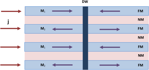
Figure 1: (Color online) Artificial AFM with the 180^∘ DW. Distribution of magnetization vectors $\mathbf{M}_{1}$, $\mathbf{M}_{2}$, (thick arrows) within each of FM sublayers is inhomogeneous, however, due to strong interlayer coupling rotation of magnetization in different layers is coherent forming the global DW (vertical stripe). Nonpolarized current $\mathbf{j}$ flows parallel to the easy axis of the layer.

In the case of current-in-plane configuration each layer – macroscopic sublattice, – can polarize the current along the local magnetization vector $\mathbf{M}_{k}$ ($k=1,\ldots,N_{\mathrm{layer}}$) thus producing a modulation of spin polarization. So, the energy density of $sd$-exchange is described with the expression (cp.(3))

$$\mathcal{H}_{\mathrm{sd}}=-\frac{J_{\mathrm{sd}}}{M_{s}N_{\mathrm{layer}}}\sum_{k=1}^{N_{\mathrm{layer}}}\mathbf{M}_{k}\mathbf{m}_{k},$$ (29)

where $\mathbf{m}_{k}$ is electron magnetization density of the $k$-th layer and $M_{s}=|\mathbf{M}_{k}|$. For a collinear structure consisting of two equivalent magnetic sublattices $\mathbf{M}_{1}$ and $\mathbf{M}_{2}$ Eq. (29) can be presented in the form analogous to (3) with $J_{\mathrm{sd}}^{\mathrm{FM}}=J_{\mathrm{sd}}^{\mathrm{AFM}}=J_{\mathrm{sd}}$

$$\mathcal{H}_{\mathrm{sd}}=-\frac{J_{\mathrm{sd}}}{4M_{s}}\left(\mathbf{m}\mathbf{M}+\mathbf{l}\mathbf{L}\right),$$ (30)

where $\mathbf{L}=\mathbf{M}_{1}-\mathbf{M}_{2}$ is AFM vector, $\mathbf{M}=\mathbf{M}_{1}+\mathbf{M}_{2}$ is macroscopic magnetization of localized spins and $\mathbf{l}$ and $\mathbf{m}$ are analogous combinations for free electrons.

If we neglect small perpendicular spin transfer between the layers, the current-induced dynamics of sublattice magnetization $\mathbf{M}_{k}$ within the sublayer ($k=1,2$) can be described with the standard equation for FM Zhang:PhysRevLett.93.127204 ; Sun:2011EPJB_79_449S :

$$\dot{\mathbf{M}}_{k}=-\gamma\left[\mathbf{M}_{k}\times\mathbf{H}^{\mathrm{eff}}_{k}\right]+\frac{\alpha_{G}}{M_{s}}\left[\mathbf{M}_{k}\times\dot{\mathbf{M}_{k}}\right]+b(\mathbf{j}\cdot\nabla)\mathbf{M}_{k}-\frac{c}{M_{s}}\left[\mathbf{M}_{k}\times(\mathbf{j}\cdot\nabla)\mathbf{M}_{k}\right],$$ (31)

where $\mathbf{H}^{\mathrm{eff}}_{k}\equiv-(\partial U/\partial\mathbf{M}_{k})$ ($U$ is the density of magnetic energy), $\alpha_{G}$ is the constant of Gilbert damping (inversely proportional to the FMR quality factor), coefficients $b=\mu_{B}P/eM_{0}(1+\xi^{2})$ and $c=b\xi$ (where $\xi\equiv\hbar/(\tau_{\mathrm{sf}}J_{\mathrm{sd}})\ll 1$) describe AST and NAST within each FM layer, correspondingly. The sign of the first term in the r.h.s. of Eq. (31) is related with the chosen positive sign of gyromagnetic ratio, $\gamma>0$.

In contrast to a single, isolated FM layer, the effective field $\mathbf{H}^{\mathrm{eff}}_{k}$ in artificial magnet includes contribution from the exchanged coupling. In particular, in the simplest case of a collinear AFM:

$$U=U_{\mathrm{AFM}}(\mathbf{L},\nabla\mathbf{L})+\frac{H_{\mathrm{ex}}}{4M_{s}}\mathbf{M}^{2},$$ (32)

where the energy density $U_{\mathrm{AFM}}(\mathbf{L},\nabla\mathbf{L})$ includes the magnetic anisotropy and contribution from inhomogeneous exchange (cp. with (19)), $H_{\mathrm{ex}}$, as above, is the constant of the exchange coupling equal to spin-flip field.

The set of Eqs. (31) can be simplified in approximation of rather strong exchange coupling between sublattices-sublayers, i.e., when the characteristic values of the external fields (including current-induced effects) are much smaller than $H_{\mathrm{ex}}$ and thus $|\mathbf{M}|\ll|\mathbf{L}|$. First, we rewrite equations (31) in terms of magnetization, $\mathbf{M}$, and AFM vector, $\mathbf{L}$, as follows:

$$\dot{\mathbf{M}} = -\gamma\mathbf{L}\times\mathbf{H}_{\mathrm{L}}+\frac{\alpha_{G}}{2M_{s}}\left[\mathbf{L}\times\dot{\mathbf{L}}\right]+b(\mathbf{j}\cdot\nabla)\mathbf{M}-\frac{c}{2M_{s}}\left[\mathbf{L}\times(\mathbf{j}\cdot\nabla)\mathbf{L}\right]$$ (33)

$$\dot{\mathbf{L}} = \frac{\gamma H_{\mathrm{ex}}}{2M_{s}}\mathbf{L}\times\mathbf{M}+b(\mathbf{j}\cdot\nabla)\mathbf{L},$$

where the effective field $\mathbf{H}_{\mathrm{L}}\equiv-(\delta U_{\mathrm{AFM}}/\delta\mathbf{L})$.

Then, following the standard approach proposed by Bar’yakhtar and Ivanov Bar-june:1979E ; Turov:1998E , we exclude magnetization $\mathbf{M}$ from the second of Eqs. (33) thus obtaining the self-consistent dynamic equation for AFM vector in the presence of current:

$$\mathbf{L} \times \left[\ddot{\mathbf{L}}-2\gamma^{2}M_{s}H_{\mathrm{ex}}\mathbf{H}_{\mathrm{L}}+\gamma H_{\mathrm{ex}}\alpha_{G}\dot{\mathbf{L}}-2b(\mathbf{j}\cdot\nabla)\dot{\mathbf{L}}\right.$$

$$- \left.b\left(\frac{d\mathbf{j}}{dt}\cdot\nabla\right)\mathbf{L}+b^{2}(\mathbf{j}\cdot\nabla)^{2}\mathbf{L}-\gamma H_{\mathrm{ex}}c(\mathbf{j}\cdot\nabla)\mathbf{L}\right]=0.$$

Corresponding Lagrange and Rayleigh functions are

$$\mathcal{L}=\frac{1}{4\gamma^{2}H_{\mathrm{ex}}M_{s}}\left(\dot{\mathbf{L}}-b(\mathbf{j}\cdot\nabla)\mathbf{L}\right)^{2}-U_{\mathrm{AFM}},$$ (35)

and

$$\mathcal{R}=\frac{\alpha_{G}}{4\gamma M_{s}}\dot{\mathbf{L}}^{2}-\frac{c}{2\gamma M_{s}}\dot{\mathbf{L}}(\mathbf{j}\cdot\nabla)\mathbf{L}.$$ (36)

As above, the Railegh function (36) is considered at fixed generalized thermodynamic forces $\nabla\mathbf{L}$.

To illustrate the peculiar features of the current-induced phenomena in artificial, or synthetic antiferromagnets (SyAFMs), we consider the simplest example of an easy-axis AFM whose dynamics can be described with the single variable $\theta$ (angle between $\mathbf{L}$ and easy axis) and the density of the direct current $\mathbf{j}\|z$. Then, dynamic Eq. (III), Lagrange(35), and Rayleigh functions (36) take the following form (cp. with their counterparts (23), (24), (25)):

$$\ddot{\theta}-bj\frac{\partial\dot{\theta}}{\partial z}-({v_{\mathrm{mag}}^{2}-b^{2}j^{2}})\frac{\partial^{2}\theta}{\partial z^{2}}-v_{\mathrm{mag}}^{2}\Delta_{\perp}\theta+\frac{\gamma^{2}}{\chi}\frac{dU_{\mathrm{an}}}{d\theta}=-2\gamma_{\mathrm{AFM}}\dot{\theta}-\frac{\gamma cjH_{\mathrm{ex}}}{2}\frac{\partial\theta}{\partial z},$$ (37)

where $U_{\mathrm{an}}$ is the density of the magnetic anisotropy energy, $\Delta_{\perp}$ is two-dimensional Laplace operator in $xy$ plane,

$$\mathcal{L}=\frac{\chi}{2\gamma^{2}}\left(\dot{\theta}-bj\frac{\partial\theta}{\partial z}\right)^{2}-\frac{\chi}{2\gamma^{2}}\left(v_{\mathrm{mag}}^{2}-b^{2}j^{2}\right)\left(\frac{\partial\theta}{\partial z}\right)^{2}-U_{\mathrm{an}}(\theta),$$ (38)

and

$$\mathcal{R}=\frac{\chi}{\gamma^{2}}\left(\gamma_{\mathrm{AFM}}\dot{\theta}^{2}-\gamma cjH_{\mathrm{ex}}\dot{\theta}\frac{\partial\theta}{\partial z}\right),$$ (39)

where $2\gamma_{\mathrm{AFM}}=\gamma\alpha_{G}H_{\mathrm{ex}}$ and $\chi=2M_{s}/H_{\mathrm{ex}}$, as above.

Comparison of Eqs. (23) and (37) shows that AST described with the constant $b=b_{\mathrm{AFM}}$ has exactly the same form in FM, AFM and SyAFM. In any type of AFM, regardless of type of $sd$-exchange, AST results in kinematic effects and reveals itself in the renormalization of the DW width (see Eq. (22)).

The main difference between AFMs with FM- and AFM-like $sd$-exchange shows in NAST (term with $c$). First of all, corresponding constants of NAST, $c_{\mathrm{AFM}}$ (see (15)) and $c$ in (31) have different dimensionality and different microscopic origin. Roughly speaking, in artificial systems (and in FMs) the NAST arises mainly from the second term in the l.h.s. of general relation (11), i.e. from rotation of free electron spins around the local magnetization. In contrast, this process is neglected in AFMs with the FM-like $sd$-exchange, as was already discussed above.

Second, while in “natural” AFMs the nonadiabatic spin torque has pure dynamic origin, i.e. is proportional to time derivatives of $\theta$, in artificial AFMs the NAST appears in the region of inhomogeneuity and is proportional to space derivative of $\theta$.

Third, in analogy with FMs, the NAST in SyAFMs can compensate the internal losses and ensure steady motion of the DW. Really, a soliton-like solution $\theta_{\mathrm{stab}}(z-v_{\mathrm{DW}}t)$ makes vanish the r.h.s. of Eq. (37) if

$$v_{\mathrm{DW}}=\frac{cj}{\alpha_{G}}=\frac{\gamma cjH_{\mathrm{ex}}}{2\gamma_{\mathrm{AFM}}}.$$ (40)

Analysis of Eq. (40) shows that the velocity of steady motion in SyAFM, in analogy with FMs and in contrast to “natural” AFMs (cp. with (28)), is proportional to the current density $j$ and is defined by the balance of damping (constant $\alpha_{G}$) and NAST (constant $c$). Expression (40) can also be interpreted in other aspect. Really, the FMR quality factor (inversely proportional to $\alpha_{G}$) is usually greater than the AFMR quality factor. This difference stems from the exchange enhancement of damping coefficient: $\gamma_{AFM}\propto\alpha_{G}H_{\mathrm{ex}}$, while $\Omega_{\mathrm{AFMR}}\propto\sqrt{H_{\mathrm{an}}H_{\mathrm{ex}}}$, so, the quality factor $\Omega_{\mathrm{AFMR}}/\gamma_{AFM}\propto\sqrt{H_{\mathrm{an}}/H_{\mathrm{ex}}}/\alpha_{G}\ll 1/\alpha_{G}$. However, in the case of SyAFM both NAST and damping are enhanced in a similar way, as seen from the second equality in (40). So, the velocity of steady motion in SyAFM has the same value as the velocity of current-induced DW motion in the FM constituents of this artificial structure. It should be also mentioned that the experiments Aliev:2009PhRvB..79m4423H point to current-induced DW motion in the SyAFM consisting of Fe/Cr multilayers.

At last, we would like to note that according to Eqs. (III) and (37) the current can set into motion the 180^∘ DW in SyAFM, while the constant magnetic field can not. Really, the 180^∘ DW separates the translation domains (with $\mathbf{L}$ and $-\mathbf{L}$) which, due to quadratic dependence of Zeeman energy ($\propto(\mathbf{H}\times\mathbf{L})^{2}$), keep equivalence in the constant magnetic field. In contrast, the staggered polarization of current in the SyAFM ensures the same direction of the ponderomotive force in each FM sublayer (see Fig.2). Thus, the current-induced motion of the DW in SyAFM is equivalent to the motion of $N_{\mathrm{layer}}$ FM domain walls synchronized due to AFM exchange coupling between the layers.

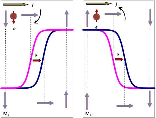
Figure 2: (Color online) Current-induced motion of 180^∘ DW in artificial AFM. Lines show the magnetization profiles $\mathbf{M}_{1}(z)$, $\mathbf{M}_{2}(z)$ within each of FM sublayers. Arrows in upper (lower) row schematically show the orientation of magnetization in different points (dashed lines) before (after) interaction with the free electron $e$. In both cases the current pushes the DW in the same direction and thus produces the same ponderomotive force $\mathbf{F}$ in each sublayer.

IV Discussion: comparison of different models

Above we obtained two forms of dynamics equations for AFM texture in the presence of current, starting from different forms of $sd$-coupling. Thus, Eqs. (16) and (III) constitute the most essential result of our paper.

Analysis of these equations shows that the continuous AFM systems, in analogy with FM textures, should demonstrate the current-induced dynamics. However, peculiarities of current-induced phenomena strongly depend upon the details of band structure and, particularly, of coupling between the spin-contributing localized electrons and carriers. We expect that in the alloys with well separated $d$- and $s$-bands (like FeMn Nakamura:PhysRevB.67.014405 or IrMn) the $sd$-exchange has the FM-like structure (2) and current-induced dynamics is modeled with Eq. (16). Current-induced effects in this case have the dynamic origin and could be observed in the moving textures or along with field- or temperature-driven oscillations of AFM vectors.

The second, AFM-like type of $sd$-exchange can be expected in artificial AFMs, where the staggered spin modulation of free electrons is imposed by the geometry of superstructure or in the itinerant AFMs like Cr (interconnection between the transport properties and AFM order in Cr was recently observed in Ref.Kummamuru:2011, ). However, applicability of $sd$-exchange model in the latter case needs further investigation.

It is instructive to compare the Eqs. (16) and (III) with the models proposed by Hals et al. Tserkovnyak:PhysRevLett.106.107206 and Swaving and Duine Duine:PhysRevB.83.054428 ; Duine:0953-8984-24-2-024223 . For this purpose we reproduce four known dynamic equations for the collinear AFM along with the short description. For the sake of clarity we change some of the original author’s notations, so that AFM order parameter (AFM, or Néel, vector) is denoted as $\mathbf{L}$, exchange constant as $J_{\mathrm{ex}}\equiv 2H_{\mathrm{ex}}M_{s}$, etc.

1. Equation (8) of Ref. Tserkovnyak:PhysRevLett.106.107206 :

   $$\ddot{\mathbf{L}} = -\widetilde{\gamma}\mathbf{L}\times\dot{\mathbf{H}}+\widetilde{\gamma}G_{1}\dot{\mathbf{H}}_{L}+\widetilde{\gamma}(\eta+G_{1}\beta)\underline{\left(\frac{d\mathbf{j}}{dt}\cdot\nabla\right)\mathbf{L}}$$ (41)

   $$+ 2\widetilde{\gamma}H_{\mathrm{ex}}M_{s}\left[\gamma\mathbf{H}_{L}-\alpha_{G}\dot{\mathbf{L}}+\underline{\gamma\beta(\mathbf{j}\cdot\nabla)\mathbf{L}}\right],$$

   where $G_{1}$ is the exchange damping parameter (omitted in our model), $\widetilde{\gamma}=\gamma/(1+G_{1}\alpha_{G})$, $\eta$ and $\beta$ parametrize AST and NAST, respectively. This equation is derived from the general thermodynamic principles starting from the hypothesis of spin pumping effect in AFMs. In other words, the main assumption of the model is that the spins of carriers flowing through AFM layer aquire the same magnetic ordering (staggered magnetization) as the localized moments. This picture is consistent with the model of artificial AFM considered in the present paper and thus, Eq. (41) should be compared with Eq. (III) derived in assumption of AFM-like $sd$-exchange:

   $$\ddot{\mathbf{L}} = 2\gamma^{2}H_{\mathrm{ex}}M_{s}\mathbf{H}_{\mathrm{L}}-\gamma\alpha_{G}H_{\mathrm{ex}}\dot{\mathbf{L}}+\underbrace{2b(\mathbf{j}\cdot\nabla)\dot{\mathbf{L}}-b^{2}(\mathbf{j}\cdot\nabla)^{2}\mathbf{L}}_{\mathrm{2nd}}$$ (42)

   $$+ \underline{b\left(\frac{d\mathbf{j}}{dt}\cdot\nabla\right)\mathbf{L}}+\underline{\gamma cH_{\mathrm{ex}}(\mathbf{j}\cdot\nabla)\mathbf{L}}.$$

   To simplify the analysis, the similar current-induced terms in both equations are underlined. The terms labeled as “2nd” in our model are of the second order of value in $\mathbf{j}$, $\dot{\mathbf{L}}$ and were omitted as small in Ref. Tserkovnyak:PhysRevLett.106.107206 . Thus, we can conclude that both models (AFM spin pumping and AFM-like $sd$-exchange models) predict the same dynamics and both work well for artificial AFMs.

2. Equation (14) of Ref. Duine:PhysRevB.83.054428 or (3) of Ref. Duine:0953-8984-24-2-024223 :

   $$\mathbf{L} \times \left(\ddot{\mathbf{L}}+\gamma_{D}\dot{\mathbf{L}}-v_{\mathrm{mag}}^{2}\nabla^{2}\mathbf{L}\right)+\frac{\partial}{\partial t}\left[\mathbf{L}\times(\mathbf{v}\cdot\nabla)\mathbf{L}\right]=$$ (43)

   $$= -\left(\mathbf{L}\cdot\dot{\mathbf{L}}\times(\mathbf{v}\cdot\nabla)\mathbf{L}\right)\mathbf{L}-v_{\mathrm{mag}}(\mathbf{r}\cdot\nabla)(\mathbf{v}\cdot\nabla)\mathbf{L}$$

   where $\mathbf{r}=(111)^{T}$, $\gamma_{D}$ is the damping parameter. This equation is derived for the structure in which the sublattice magnetization rotates from site to site, i.e. sublattice magnetizations $\mathbf{M}_{1}$, $\mathbf{M}_{2}$ are tilted with respect each other even in the absence of field and current. This gives rise to a Lifshitz-like contribution $\partial\mathbf{L}/\partial z$ to magnetization (see Eq. (12) of Ref. Duine:PhysRevB.83.054428, ) typical for noncentrosymmetric incommensurate structures. The current-induced effects in this model arise from the noncompensated static magnetization omitted in both our models and in Ref. Tserkovnyak:PhysRevLett.106.107206 . It should be also stressed that l.h.s. of Eq. (43) should be orthogonal to $\mathbf{L}$ and this condition imposes additional limitations on the type of space inhomogeneuity.

3. Equation (16) derived from spin conservation principle assuming FM-like $sd$-exchange and adapted for the collinear AFM with two magnetic sublattices by substitution $\boldsymbol{\Omega}\rightarrow\mathbf{L}\times\dot{\mathbf{L}}$ and due account of orthogonality condition $(\mathbf{M}_{\mathrm{AFM}}\cdot\mathbf{L})=0$:

   $$\mathbf{L} \times \left\{\ddot{\mathbf{L}}-2\gamma^{2}H_{\mathrm{ex}}M_{s}\mathbf{H}_{\mathrm{L}}+\gamma\alpha_{G}H_{\mathrm{ex}}\dot{\mathbf{L}}\right\}$$

   $$= b_{\mathrm{AFM}}\left\{(\mathbf{j}\cdot\nabla)\left(\mathbf{L}\times\dot{\mathbf{L}}\right)-\mathbf{L}\left[\mathbf{L}\cdot(\mathbf{j}\cdot\nabla)\mathbf{L}\times\dot{\mathbf{L}}\right]/4M_{s}^{2}\right\}$$

   $$+ (c_{\mathrm{AFM}}/4M_{s}^{2})\left\{2\dot{\mathbf{L}}[\dot{\mathbf{L}}\cdot\mathbf{L}\times(\mathbf{j}\cdot\nabla)\mathbf{L}]+4M_{s}^{2}\ddot{\mathbf{L}}\times(\mathbf{j}\cdot\nabla)\mathbf{L}+\mathbf{L}[\ddot{\mathbf{L}}\cdot\mathbf{L}\times(\mathbf{j}\cdot\nabla)\mathbf{L}]\right\}.$$

   Comparison of Eq. (3) with Eqs. (41) and (42) shows that current-induced terms and, consequently, current-induced phenomena predicted within two models of $sd$-exchange are absolutely different. This difference opens a way to elucidate the mechanism of $sd$-coupling in AFM materials from the peculiarities of current-induced dynamics.

V Conclusions

To summarize, we considered the current-induced dynamics for different types of the continuous AFMs and obtained equations that could be used for the analysis of the dDWs, droplets and other soliton-like structures in AFMs in the presence of current. The predicted qualitative difference in dynamics for FM- and AFM-like types of $sd$-exchange opens a way for experimental investigation of the carrier’s role in AFM ordering of a certain material.

- (1) J. Slonczewski, J. Magn. Magn. Mater. 159, L1 (1996)
- (2) L. Berger, Phys. Rev. B 54, 9353 (1996)
- (3) S. Zhang and Z. Li, Phys. Rev. Lett. 93, 127204 (2004)
- (4) P. M. Haney and A. H. MacDonald, Phys. Rev. Lett. 100, 196801 (2008)
- (5) Z. Wei, A. Sharma, A. S. Nunez, P. M. Haney, R. A. Duine, J. Bass, A. H. MacDonald, and M. Tsoi, Phys. Rev. Lett. 98, 116603 (2007)
- (6) H. V. Gomonay and V. M. Loktev, Phys. Rev. B 81, 144427 (2010)
- (7) H. V. Gomonay, R. V. Kunitsyn, and V. M. Loktev, Phys. Rev. B 85, 134446 (2012)
- (8) A. Nunez, R. Duine, P. Haney, and A. MacDonald, Phys. Rev. B 73, 214426 (2006)
- (9) A. F. Andreev and V. I. Marchenko, Physics-Uspekhi 23, 21 (1980)
- (10) Y. Endoh, G. Shirane, Y. Ishikawa, and K. Tajima, Solid State Commun. 13, 1179 (1973)
- (11) W. Kuch, L. I. Chelaru, F. Offi, J. Wang, M. Kotsugi, and J. Kirschner, Phys. Rev. Lett. 92, 017201 (2004)
- (12) Z. Z. Sun, J. Schliemann, P. Yan, and X. R. Wang, Eur. Phys. Jour. B 79, 449 (Feb. 2011)
- (13) S. V. Vonsovskii, Magnetism (Wiley and Sons, Incorporated, John, 1974)
- (14) V. G. Bar’yakhtar, JETP 60, 863 (1984)
- (15) K. M. D. Hals, Y. Tserkovnyak, and A. Brataas, Phys. Rev. Lett. 106, 107206 (Mar 2011)
- (16) Y. B. Bazaliy, B. A. Jones, and S.-C. Zhang, Phys. Rev. B 57, R3213 (1998)
- (17) A.M.Kosevich, B.A.Ivanov, and A.S.Kovalev, Nonlinear magnetization waves. Dynamical and topological solitons (Naukova Dumka, Kiev, 1983) 189 p.(in Russian)
- (18) I. Bar’yakhtar and B. Ivanov, Sov. J. of Exper. Theor. Phys. 58, 190 (1983)
- (19) O. Hellwig, A. Berger, and E. E. Fullerton, Phys. Rev. Lett. 91, 197203 (Nov 2003)
- (20) D. Herranz, R. Guerrero, R. Villar, F. G. Aliev, A. C. Swaving, R. A. Duine, C. van Haesendonck, and I. Vavra, Phys. Rev. B 79, 134423 (2009)
- (21) R. Sbiaa, S. N. Piramanayagam, and R. Law, Appl. Phys. Lett. 95, 242502 (2009)
- (22) A. Hashimoto, S. Saito, K. Omori, H. Takashima, T. Ueno, and M. Takahashi, Appl. Phys. Lett. 89, 032511 (2006)
- (23) Y. Xiao, S. Chen, Z. Zhang, B. Ma, and Q. Y. Jin, J. Appl. Phys. 113, 17A325 (2013)
- (24) O. Hellwig, T. L. Kirk, J. B. Kortright, A. Berger, and E. E. Fullerton, Nature Mater 2, 112 (2003)
- (25) N. Kiselev, U. Rößler, A. Bogdanov, and O. Hellwig, J. Magn. Magn. Mater. 322, 1340 (2010)
- (26) I. Bar’yakhtar and B. Ivanov, Sov. J. Low Temp. Phys. 5, 361 (1979)
- (27) E. A. Turov, A. V. Kolchanov, V. V. Men’shenin, I. F. Mirsaev, and V. V. Nikolaev, Uspekhi Fizicheskikh Nauk 168, 1303 (1998)
- (28) K. Nakamura, T. Ito, A. J. Freeman, L. Zhong, and J. Fernandez-de Castro, Phys. Rev. B 67, 014405 (2003)
- (29) Y. Soh and R. Kummamuru, Philos Transact A Math Phys Eng Sci. 369, 3646 (2011)
- (30) A. C. Swaving and R. A. Duine, J. Phys. Cond. Matt. 24, 024223 (2012)
- (31) A. C. Swaving and R. A. Duine, Phys. Rev. B 83, 054428 (2011)
- (32) I. Bar’yakhtar and B. Ivanov, Solid State Comm. 34, 545 (1980)