Positronium decay in a circular polarized laser field

Abstract

We calculate the lifetime of both the o-Ps and the p-Ps positronium annihilation decay $Ps\to\gamma\gamma$ in the strong circular polarized laser field. We take a strategy of the factorization to separate the effects caused by the Coulomb interaction and the strong laser field interaction. It is factorized in the time direction but not in the space direction. Our results show that in the laser with long wavelength and high intensity, the lifetimes of those Ps states are dramatically increased. For $\rm CO_{2}$ laser with $10\,\mu m$ wavelength and $10^{13}W/cm^{2}$ intensity, lifetime of the spin-single positronium is increased by $10^{8}$ times. Our result is consistent with those obtained by solving the Schödinger equation. This effect may be useful for the high harmonic generation(HHG) effects provided with the Pskeitel2004 .

I Introduction

The fast technological advance in the past decades brings us the high-power laser systems with peak intensities up to $10^{22}W/cm^{2}$laserintensity22 , and one would expect a further increase in the near future275004 . Such high-power laser systems lead to studies of the fundamental processes of quantum electrodynamics in the presence of a strong laser field realistic in experiments. Some typical processes are laser-induced Comptom scatteringcompton , laser-assisted Mott scatteringMott , laser-assisted M$\phi$ller scattering Moller1 ; moller2 and laser-assisted Bhabha scatteringBhabha , bremsstrahlungbremsstrahlung . The mechanism of production of $e^{+}e^{-}$ pair creation by a projectile particle colliding with an intense laser beam is widely studied both theoretical and experimental, and first directly observed at SLAC facility46.6 .

Positronium(Ps), the electron-positron bound state under attractive Coulomb interactions, is well suitable for probing many fundamental aspects of particle physics. For the Ps in vacuum, there are three distinct energy scales: the electron mass $m$, the three-momentum $m\alpha$ and the binding energy $m\alpha^{2}$. The lowest $S-$wave state can be spin-singlet para-positronium(p-Ps) or spin-triplet ortho-positronium(o-Ps). The binding energy of these two states is $1/2\,m\,\alpha^{2}=6.8eV$. They can decay into even or odd hard photons, respectively, via spontaneous annihilation. The spin 0 singlet state annihilates into two photons with the lifetime of $1.25\times 10^{-10}$ second while the spin one triplet decay only into three photons with a lifetime of $1.4\times 10^{-7}$ second.

Under strong laser fields, besides the annihilation decay, the Ps may also decay via ionization. The ionization of normal atoms under laser is described by the Keldysh’s theoryKeldysh . In laser electro-magnetic (EM) field, the charged particles receive the ponderomotive motion along the laser beam direction which is a nonlinear effects of the EM interaction of the electrons and the laser beam. For normal atoms, they are ionized since the nucleus and the electrons gain very different velocities because their masses are very different. However, for the Ps, the ionization is quite different from that of the normal atoms for the reason that both the electron and the positron in the Ps receive the same ponderomotive momentum along the laser beam direction since they possess the same mass. Consequently, the Ps is much harder to be ionized than the normal atoms under the high laser EM field. This feature is suggested to produce HHG by the Ps statekeitel2004 . To make this mechanism work, it is required that this has enough lifetime. Thus it is essential to calculate the partial lifetime of the annihilation process.

Under strong laser EM fields, the annihilation partial decay width of the Ps may be changed. Intuitively, with the laser field, the electron and the positron move back and forward periodically in the perpendicular direction of the laser beam. It effectively reduces the wavefunction at origin and enhances the lifetime of the Ps. Unlike in vacuum, in laser EM fields, both the o-Ps and the p-Ps can decay into two gamma photons. Meanwhile the Ps annihilation may produce a single photon. To precisely predict the lifetime of the Ps, one needs to solve the dynamics of the system combining Coulomb potential, the laser potential and the annihilation process together, which is very complicated. To carry out calculations, certain approximations are necessary.

In Refs.Ehlotzky Brazil , the authors studied the nonperturbative effects of intense laser field on the origin of the wavefunction by solving Schödinger equation (SCHE). They started from a time-dependent SCHE with Coulomb interaction and the dipole interaction for the laser EM field which is reasonable since the wavelength of the laser photon is much larger than the typical size of the Ps. With some additional approximations they derive a time-independent local SCHE with the dynamics similar to the $\rm H_{2}^{+}$ ion. By using variational method, they can approximately solved the equation. Their method is available only for the linearly polarized laser field.

In this paper we reconsider the Ps decay processes into two photons in circular polarized laser field with higher intensity by examining the energy scales involved in the annihilation decay processes. Notice that besides two produced hard photons, there are a set of laser photons are emitted or absorbed from the laser sources. Thus the basic annihilation processes can be described as:

$$e^{+}+e^{-}\to\gamma+\gamma\pm n\,\gamma_{k}\;,$$ (1)

where $\pm n$ is the number of emitted or absorbed laser photon $\gamma_{k}$ with momentum $k=(\omega,{\rm\bf k})$. When the typical $n$ satisfying $n\omega$ much larger than the binding energy of the bound state, the typical kinetic energy of the relative motion in the rest frame of the $e^{+}e^{-}$ system is then much larger than the Coulomb potential energy. Hence the Coulomb potential interaction can be negligible in the leading order approximation in calculating this annihilation process. In this way, the effects of the annihilation decay process (1), as a short-distance effect, is factored out from the long-distance effects which is governed by Coulomb interaction. This factorization is different from the conventional factorization. It is factorized in the time direction but not in the space direction since they are in the compatible size in the space direction.

The short-distance effect can be calculated by perturbation theory. It is different from the usual perturbation theory in vacuum. Here one has to include contributions arising from this background EM field. To this end, we take Volkov state to describe the electron and the positron under the classic laser EM fieldVolkov . To carry our calculations, we also use the propagator of the electron and the positron under the laser EM background field obtained by Schwinger proper-time method. Our strategy is in the spirit of the NRQED factorization formula, which is the QED version of NRQCD factorization formulaBBL for strong interaction without laser field background. Our results are suitable for the case that the motions of the positron and the electron caused by the laser field is relativistic. Moreover, one advantage of our method is that it can be used to calculate various differential distributions of the final hard photons. In addition, it can be applied to the case of circular polarization laser.

The remainder of this paper is organized as follows. In Sec. II, we propose a factorization formula to carry out calculations on the processes. In Sec. III, we present numerical results. Sec.IV is dedicated to a brief summary and conclusions. Throughout this paper, we use natural units with $\hbar=c=1$. The fine structure constant is $\alpha=\frac{e^{2}}{4\pi}\approx\frac{1}{137}$.

II Theoretical Framework

In this section, we calculate the decay rate of the Ps into double hard photons in a strong laser EM field.

The process can proceed at the second order in the QED hard interaction with momentum transfer at order of $m$ or higher. There are two Feynman diagrams contributing to the process as shown in Fig. 1. For the photons with momenta $k_{1}$ and $k_{2}$ and corresponding polarization vectors $\mbox{\boldmath$\epsilon$}_{1}$ and $\mbox{\boldmath$\epsilon$}_{2}$, respectively, the S-matrix elements can be written as

$$S_{Ps\to\gamma\gamma} = -e^{2}\;{\epsilon_{1\mu}\epsilon_{2\nu}}\;\int d^{4}x_{1}\,d^{4}x_{2}\;e^{i\,k_{1}x_{1}+i\,k_{2}x_{2}}$$ (2)

$$\times \langle 0|\,\left[\,\bar{\Psi}\left({x_{1}}\right)\,\gamma^{\mu}\,S\left({x_{1}},{x_{2}}\right)\,\gamma^{\nu}\Psi\left({x_{2}}\right)\,+\,\bar{\Psi}\left({x_{2}}\right)\,\gamma^{\nu}\,S\left({x_{2}},{x_{1}}\right)\,\gamma^{\mu}\Psi\left({x_{1}}\right)\,\right]\,|Ps\rangle\;,$$

where $\Psi(x)$ and $S\left({x_{1}},{x_{2}}\right)$ are the four-fermion field and the propagator of the electrons under the Coulomb interaction and the laser EM field. They satisfy Dirac Equation

$$(i\not\!\!{D}-m)_{x}\;\Psi(x)=0\;,$$ (3)

and

$$(i\not\!\!{D}-m)_{x}\;S(x,y)=\delta^{4}(x-y)\;,$$ (4)

respectively, where $D_{\mu}=\partial_{\mu}+ieA_{\mu}$. Here the vector potential $A_{\mu}$ consists of Coulomb potential and the laser EM potential. The laser EM potential appearing here implies that arbitrary number laser photons can be absorbed or emitted by the electron and the positron. Generally, these equations are difficult to be solved analytically. Here our strategy is to disentangle the long distance effects and the short distance effects. Notice that in the case of the laser field absent, the annihilation of the electron and the positron is the short-distance effect while the formation of the bound state is the long-distance effect. They are separated well and factorizable. When the laser field appear, the fermion line will emit or absorb a number of laser photons from the laser source. Including these photons, the real annihilation process is the one given in Eq. (1). The stronger of the laser field is, the larger the typical $n$ is. If the laser field is sufficiently strong so that $n\omega$ is much larger than the binding energy of the positronium, the electron or the positron gain typical kinetic energy (either with plus sign or with minus sign) of the relative motion in the rest frame of the $e^{+}e^{-}$ system being much larger than the Coulomb potential energy. Hence the contribution from the Coulomb potential interaction can be negligible in calculating the interaction field by Eq. (3) and the propagator by Eq. (4) appearing in Eq. (2). In the diagrammatic language, the bound state of the Ps is formed by exchanging Coulomb interactions. One has to resum over all those diagrams since each of them give the same order contribution to the binding energy. Specifically, the Coulomb singularity contribution ($1/v\sim 1/\alpha$ ) arising from each Coulomb photon exchange is compensated by the coupling constant $\alpha$ from one more exchange. Once $n\omega$ is much larger than the binding energy of the positronium, the electron or the positron are far away from the Coulomb region with momentum $(m\alpha^{2},m\alpha)$, the Coulomb singularity appears no longer while the coupling is still there. Thus one more such exchange of the ladder is suppressed by a factor of $\alpha$, hence perturbatively calculable. In the leading order approximation, one may just neglect it. Therefore, in solving the Dirac Eq. (3) and the propagator by Eq. (4), one may neglect the Coulomb interactions once the typical value of $n$ satisfies $n\omega\gg m\alpha^{2}$ and then the calculation can be simplified significantly. This is just the case we are concerning in this paper. In this way, the long-distance effects caused by the Coulomb interaction in the annihilation process are factored out. However, this factorization is different from the conventional factorization. It is factorized in the time direction but not in the space direction since they are in the same size in the space direction. With only the laser EM field, those equations can readily be solved.

We assume the laser propagates along the $z$ direction with photon momentum $k^{\mu}=\omega(1,0,0,1)$ and the vector potential $A$ possesses only transverse components. For a circular polarized laser, the vector potential can be written as:

$$A^{\mu}(x)=a^{\mu}_{1}\cos\xi+a^{\mu}_{2}\sin\xi\,$$ (5)

where $a^{\mu}_{1}=a(0,1,0,0)$, $a^{\mu}_{2}=a(0,0,1,0)$ , $a_{1}\cdot a_{2}=0$, $\xi=k\cdot x$. Thus $a$ denotes the amplitude of the vector potential. For the circular polarized laser, one has $A^{2}=-a^{2}$.

One useful dimensionless parameter describing nonlinear effects is $\eta$ which is defined as:

$$\eta\equiv\frac{e\,a}{m}\;.$$ (6)

For an electron or positron with momentum $p$ moving in an external electromagnetic field, its average effective momentum reads:

$$q=p+\frac{e^{2}\,a^{2}\,k}{2k\cdot p}=p+\frac{\eta^{2}\,m^{2}}{2k\cdot p}\,k\;.$$ (7)

Here the second term is called as ponderomotive momentum. It is proportional to $a^{2}$ and hence represents a nonlinear effect. With this momentum one may define an effective mass for the electron or the positron by:

$$m_{*}^{2}=q^{2}=m^{2}+e^{2}a^{2}=(1+\eta^{2})m^{2}\;.$$ (8)

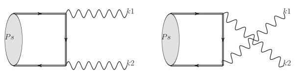
Figure 1: Feynman diagrams for $Ps\to\gamma\gamma$ in a laser field.Double lines correspond to the electron(positron) Volkov state

The wavefunction of the electron $\Phi(x,p)$ or the positron $\Phi^{\prime}(x,p)$ is given by the Volkov solutionVolkov of the classic Dirac equation For circular polarization, it reads:

$$\Phi(x,p) = e^{iS_{-}[\psi]}\,\left(1-\frac{e\,/\!\!\!k\,/\!\!\!{A}}{2\,kp}\right)\;u(p)$$ (9)

$$\equiv \Gamma(x,p)u(p)\;,$$

$$\Phi^{\prime}(x,p) = e^{iS_{+}[\psi]}\,\left(1+\frac{e\,/\!\!\!k\,/\!\!\!{A}}{2(kp)}\right)\;v(p)$$ (10)

$$\equiv \Gamma(x,p)v(p)\;,$$

where

$$S_{\pm}[\psi] = \pm(qx)+\frac{e(pa_{1})}{kp}\sin(kx)-\frac{e(pa_{2})}{kp}\cos(kx)$$ (11)

$$\Gamma_{\pm}(x,p) = \sum_{s=-\infty}^{\infty}\exp[\pm i(qx-sk)x]\Big{[}B_{s}^{0}(\alpha_{1}^{\pm},\alpha_{2}^{\pm})$$ (12)

$$+\frac{ea\,/\!\!\!k}{2k\cdot p}\left[\,/\!\!\!\epsilon_{1}B_{s}^{1}(\alpha_{1}^{\pm},\alpha_{2}^{\pm})+\,/\!\!\!\epsilon_{2}B_{s}^{2}(\alpha_{1}^{\pm},\alpha_{2}^{\pm})\right]\Big{]}\;,$$

where

$$B_{s}^{0}(\alpha_{1},\alpha_{2}) = \sum_{n=-\infty}^{+\infty}i^{n}J_{s-n}(\alpha_{1})J_{n}(\alpha_{2})$$

$$B_{s}^{1}(\alpha_{1},\alpha_{2}) = \frac{1}{2}[B_{s-1}^{0}(\alpha_{1},\alpha_{2})+B_{s+1}^{0}(\alpha_{1},\alpha_{2})]$$

$$B_{s}^{2}(\alpha_{1},\alpha_{2}) = \frac{1}{2i}[B_{s-1}^{0}(\alpha_{1},\alpha_{2})-B_{s+1}^{0}(\alpha_{1},\alpha_{2})]$$

The generalized Bessel functions are given by sums over products of the first kind.Similar treatment could be found in bremsstrahlung . The arguments of the generalized Bessel functions are defined by $\alpha_{1}^{\pm}=\pm e\frac{p_{\pm}\cdot a_{1}}{k\cdot p_{\pm}}$ and $\alpha_{2}^{\pm}=\mp e\frac{p_{\pm}\cdot a_{2}}{k\cdot p_{\pm}}$. The electron spinors are used in the following form:

$$u_{p}=\sqrt{\frac{E+m}{2E}}\left(\begin{array}[]{c}\zeta\\ \frac{\mathbf{p}\cdot\mathbf{\sigma}}{E+m}\zeta\\ \end{array}\right)\;\;\;v_{p}=\sqrt{\frac{E+m}{2E}}\left(\begin{array}[]{c}\frac{\mathbf{p}\cdot\mathbf{\sigma}}{E+m}\chi\\ \chi\\ \end{array}\right)$$ (17)

with the standard vector $\mathbf{\sigma}$ being composed of the Pauli $2\times 2$ spin matrices and $\zeta,\chi$ are two-component Pauli spinors. $p$ is the momentum of the particle outside the laser field.

The quantum field of Dirac equation can then be expressed as a superposition of the product of creation or annihilation operators and Volkov solution at momentum $p$, instead of the plane wave solutions for free particles.

The propagator of the electron in the laser background field can be obtained by Fock-Schwinger proper time methodzuber . In a circularly polarized plane it reads:

$$S_{A}(x,x^{\prime})=\left[\,i\,/\!\!\!\partial_{x}-e\,/\!\!\!A(x)+m\,\right]\,(-i)\int_{-\infty}^{0}d\tau~{}U(x,x^{\prime};\tau)$$ (18)

with

$$U(x,x^{\prime};\tau) = -\frac{i}{(4\pi)^{2}\tau^{2}}\exp~{}i\Big{[}\frac{(x-x^{\prime})^{2}}{4\tau}+\big{(}\,m_{*}^{2}+\frac{ea}{2}\phi^{1}_{\rho\nu}\sigma^{\rho\nu}\frac{\cos\xi_{1}-\cos\xi_{2}}{\xi_{1}-\xi_{2}}$$ (19)

$$+\frac{ea}{2}\phi^{2}_{\rho\nu}\sigma^{\rho\nu}\frac{\sin\xi_{1}-\sin\xi_{2}}{\xi_{1}-\xi_{2}}-i\epsilon\,\big{)}\tau-e\int^{x}_{x^{\prime}}dy_{\mu}A^{\mu}(y)\Big{]}$$

with $\phi_{\rho\nu}=k_{\mu}\epsilon_{\nu}-k_{\nu}\epsilon_{\mu}$, $\sigma^{\rho\nu}=\frac{i}{2}[\gamma_{\mu},\gamma_{\nu}]$. Performing U’s Fourier transform and integrating $\tau$, we can evaluate the electron propagator.

With Volkov solution given in (9), (10)and the propagator(18), the effects caused by the laser EM field can be explicitly extracted out. Substituting them into Eq .(2), it follows that:

$$S_{Ps\to\gamma\gamma} = ie^{2}\,\;\int d^{4}x_{1}\,d^{4}x_{2}\;e^{i\,k_{1}x_{1}+i\,k_{2}x_{2}}$$ (20)

$$\int\frac{d^{3}{\rm\bf q}}{(2\pi)^{3}}\tilde{\Phi}(\mathbf{p})Tr\{\hat{\Gamma}(x,p_{+})(\,/\!\!\!\epsilon_{1}S_{A}(x_{1},x_{2})\,/\!\!\!\epsilon_{2}$$

$$+\,/\!\!\!\epsilon_{2}S_{A}(x_{1},x_{2})\,/\!\!\!\epsilon_{1})\Gamma(x,p_{-})\Pi_{s}\}\;.$$

and $\Phi(x,p)$, $\Phi^{\prime}(x,p)$ are the Ps radial wave function in the momentum space and projection operators which are given by:

$$\Pi_{0}(P) = \frac{1}{\sqrt{m}}\,\gamma_{5}\,(\,/\!\!\!P+2m)\;,$$ (21)

for the spin-singlet case

$$\Pi_{1}(P) = \frac{1}{\sqrt{m}}\,\not\!\!\epsilon\,(\,/\!\!\!P+2m)\;,$$ (22)

for the spin-triplet state with polarization $\epsilon$.

We assume the ground state Ps atom be initially at rest. The bound state is a linear superposition of products of free states $\Psi_{p_{\pm}}$ for the electron and positron with definite relative momenta $\mathbf{q}$, which is weighted by the wavefunction $\tilde{\Phi}(\mathbf{q})$. In the momentum space, the wavefunction of the $S-$ wave reads:

$$\tilde{\Phi}(\mathbf{q})=\frac{8\pi a_{0}^{3/2}}{[1+a_{0}^{2}\mathbf{q}^{2}]^{2}}\;$$ (23)

where $a_{0}$ is the Ps radius.

To carry out integration over the relative momentum $\tilde{\Phi}(\mathbf{q})$, we ignore $\tilde{\Phi}(\mathbf{q})$ in those terms which are insensitive to $\mathbf{q}$ and keep those terms which are sensitive to $\mathbf{q}$. The amplitude can be expressed as the overlap integrals of the wave function and those terms sensitive to $\mathbf{q}$ with the generic form:

$$\phi=\sum_{r=-\infty}^{\infty}\int\frac{d^{3}{\rm\bf q}}{(2\pi\,\sqrt{a_{0}})^{3}}\tilde{\Phi}(\mathbf{q})B_{r}^{0}(\alpha_{+},\alpha_{-})\;.$$ (24)

This means that the factorization here is different from the conventional factorization. Besides the wavefunction, there is sensitive $\mathbf{q}$ dependence arising from Volkov state wavefunction as expected. It is factorized in the time direction but not in the space direction since they are in the same size in the space direction. Actually the electron and the positron in Volkov states absorb or emit $s^{-}$ and $s^{+}$ laser photons respectively in this process, corresponding to Bessel function$J_{s^{-}}(\alpha_{-})$ and $J_{s^{+}}(\alpha_{+})$. The Bessel functions decrease very quickly if $\mid s^{\pm}\mid>\mid\alpha_{\pm}\mid$. In our case we find $\mid s^{\pm}\omega\mid\ll\mid m\mid$, so we may take an approximation

$$\delta(q_{+}+q_{-}-k_{1}-k_{2}+nk)\simeq\delta(q_{+}+q_{-}-k_{1}-k_{2}).$$ (25)

With this approximation, we can reduce the infinite sum over the product of the Bessel function of the electron and the Bessel function of the positron to a single Bessel function as shown in Appendix. Finally, we can express it as

$$\phi=\frac{16}{(2\pi a_{0}^{1/2})^{3}}\int_{0}^{+\infty}dq_{z}\int_{0}^{+\infty}q_{\bot}dq_{\bot}\int_{0}^{\frac{\pi}{4}}d\varphi\tilde{\Phi}(\mathbf{q})\exp{\frac{im\eta q_{\bot}\sin\varphi}{\omega\sqrt{m^{2}+q_{\bot}^{2}+q_{z}^{2}}+q_{z}}}\;.$$ (26)

In the nonrelativistic limit, the factor in the exponential of the integrant is simplified as $i\frac{\eta}{\omega}\,q_{\bot}\sin\varphi$. If the integration is from $0$ to $2\pi$, the the overlap integral $\phi$ is nothing but Fourier transformation of the wavefunction in momentum space, i.e., the wavefunction in coordinator space at distance $\frac{\eta}{\omega}$ away from the origin along the $q_{\bot}$ axes. For the Ps, it is proportional to $e^{-\frac{\eta}{2\omega a_{B}}}$ with $a_{B}$ being the Bohr radius. This exponential suppression factor is in agreement with the result given in Brazil for the linear polarized laser, where the authors obtained their results by taking a lot of approximations. But for the exact expression given here, the integration bound is from $0$ to $\pi/4$.

From this expression, we can evaluate $\phi$ in (24) numerically. With this numerical value we calculate the $S$-matrix element analytically.

The differential decay width can then be expressed as

$$d\Gamma=\frac{1}{16\pi^{2}}\;|S_{Ps\rightarrow 2\gamma}|^{2}\;\frac{d^{3}k_{1}}{2\omega_{1}}\,\frac{d^{3}k_{2}}{2\omega_{2}}\,\delta^{(4)}(q_{+}+q_{-}-k_{1}-k_{2}+nk)\;$$ (27)

We carry out the phase space integration $\int\Pi$ by virtual of the $\delta$-function $\delta^{4}(q_{+}+q_{-}-k_{1}-k_{2})=\delta(q_{+}^{0}+q_{-}^{0}-k_{1}^{0}-k_{2}^{0})\delta^{3}(\mathbf{q_{+}}+\mathbf{q_{-}}-\mathbf{k_{1}}-\mathbf{k_{2}})$ and the relations $d^{3}k_{2}=\omega_{2}^{2}d\omega_{2}d\Omega$ . Integrating over $d^{3}\mathbf{k_{2}}$ and $dk_{1}^{0}$ we find that the phase space integral can be expressed as

$$\int\Pi = \frac{d^{3}k_{1}}{2\pi^{3}}\frac{1}{2\omega_{1}}\frac{d^{3}k_{2}}{2\pi^{3}}\frac{1}{2\omega_{2}}$$ (28)

$$\approx \frac{1}{16\pi^{2}}\int d\Omega\frac{\omega_{1}}{2Eq+\frac{2e^{2}a^{2}}{Eq}(1-\cos\theta)}$$ (29)

where $\theta$is angle between photon $\gamma_{1}$ and the laser beam direction, and

$$\omega_{1} = \frac{2E^{3}+2E\eta^{2}m^{2}}{2E^{2}+\eta^{2}m^{2}-\eta^{2}m^{2}\cos\theta}$$

Finally, we obtain the differential distribution over $\cos\theta$. For the spin-singlet state, it reads:

$$\frac{d\Gamma^{cir}(\text{p-Ps})}{d\cos\theta}=\frac{\phi^{2}}{\pi^{4}}\Gamma_{0}(\text{p-Ps})\Big{[}1+\left(\frac{3\cos\theta}{2}-\frac{5}{2}\right)\eta^{2}\Big{]}\;,$$ (30)

and for the spin-triplet state, it reads:

$$\frac{d\Gamma_{0}^{cir}(\text{o-Ps})}{d\cos\theta} = \frac{\phi^{2}}{\pi^{4}}\Gamma_{0}(\text{p-Ps})\Big{(}\cos^{2}\theta+7\Big{)}\eta^{2}\;.$$ (31)

Integrating out $\theta$ angle, one obtain the total decay rate.

$${d\Gamma^{cir}(\text{p-Ps})} = \frac{\phi^{2}}{\pi^{4}}\Gamma_{0}(\text{p-Ps})\Big{[}1-\frac{5}{2}\eta^{2}\Big{]}\;,$$ (32)

and for the spin-triplet state, it reads:

$$\frac{d\Gamma_{0}^{cir}(\text{o-Ps})}{d\cos\theta} = \frac{\phi^{2}}{\pi^{4}}\Gamma_{0}(\text{p-Ps})\,9\eta^{2}\;.$$ (33)

where $\Gamma_{0}(\text{p-Ps}\rightarrow\gamma\gamma)$ is the two-photon decay width of the spin-single $1^{1}S_{0}$ Ps state in vacuum. It reads:

$$\Gamma_{0}(\text{p-Ps}\longrightarrow\gamma\gamma)=\frac{\alpha^{5}m_{e}}{2}\;.$$ (34)

Eqs. (30)-(33) are our final results. $\Gamma$ from these equations we see that once we evaluate value of $\phi$, we can make predictions for the lifetime of the Ps in the laser EM field.

III RESULTS AND DISCUSSION

In this section, we use Eqs. (26), (30)-(33) derived in the last section to calculate the decay rate of the Ps states in the strong laser EM field. The only unknown parameter we need to calculate numerically is the overlap integral $\phi$. As argued above, the electron and the positron make period movement along the electric field provided by the laser. This efficiently reduces the value of the wavefunction at origin. As discussed in the last section, to some extent, this value is related to the wavefunction somewhere away from the origin for the Ps with laser EM fields. In the positronium case, it is exponentially suppressed comparing to the wavefunction at origin. This exponential factor governs the enhancement of the lifetime of the Ps states. The factor in the exponential is proportional to the product of the wavelength squared and the square root of the intensity of the laser field. Therefore, it is more efficient to enhance the lifetime of the positronium by increasing the wavelength than increasing the intensity of the laser. For comparison with the result given inBrazil , we first evaluate Ti:sapphire ($f=380$ THz) laser source with intensity $10^{13}$ ${\rm W/cm^{2}}$. The result given in Brazil is that the lifetime of the p-Ps state is enhanced by $641$ times while our result for this number is $3.41\times 10^{3}$. Their result is about 5 times smaller than our one. Considering the fact that this enhancement is exponential function and any tiny change of small factor will change this result dramatically this difference is not very suppressing.

We now turn to look at the case with the fixed laser photon energy at 1 eV but various intensities. Our results are listed in I.

Table 1: The enhanced factor for the lifetime of the p-Ps and the o-Ps state in the laser field with 1 eV laser photon and various value of $\eta$

$\eta$	$\Gamma_{0}(\text{p-Ps})/\Gamma_{L}(\text{p-Ps})$	$\Gamma_{0}(\text{p-Ps})/\Gamma_{L}(\text{o-Ps})$
$0.01$	54	$7.35\times 10^{4}$
$0.05$	454	$2.5\times 10^{4}$
$0.1$	3630	$5.1\times 10^{4}$

Finally we turn to look at the case with the fixed laser photon energy with $10^{13}\;{\rm W/cm^{2}}$ intensity and wavelength at $1\,\mu m$ and $10\;\mu m$ for the p-Ps state. Our results are listed in II. We see that for the wavelength at $10\;\mu m$, the lifetime of the $p-Ps$ state enhanced by a factor $10^{8}$.

Table 2: The enhanced factor for the lifetime of the p-Ps states in the laser field with $10^{13}\;{\rm W/cm^{2}}$ intensity and various wavelength

$\lambda(\mu m)$	$\Gamma_{0}$($/\Gamma{L}$)	Lifetime$(s)$
$1$	$4.7\times 10^{3}$	$5.96\times 10^{-7}$
$10$	$1.3\times 10^{8}$	$1.5876\times 10^{-2}$

IV Summary

In this paper, we calculate the partial lifetime of both the o-Ps and the p-Ps positronium annihilation decay $Ps\to\gamma\gamma$ in the strong circular polarized laser EM field. We take a strategy of the factorization to separate the effects caused by the Coulomb interaction and the strong laser field. This factorization is different from the conventional factorization. It is factorized in the time direction but not in the space direction since they are at the same size in the space direction. In calculating the short-distance effects, we use the solution of classic Dirac equation in the laser EM background field, i,e., the so-called Volkov state. We also have adopted Fock-Schwinger proper time method. we expand the Volkov solutions in plane wave in terms of the generalized Bessel function. Our results show that for long-wavelength laser with sufficiently high value of $\eta$ parameter which characterize the nonlinear effects of the laser assisted process, the lifetimes of those Ps states are dramatically increased. This is qualitatively consistent with that given in Brazil . This effect may be very useful for the HHG effects by the Pskeitel2004 .

Appendix A GENERALIZED BESSEL FUNCTIONS

Bessel functions of the first kind $J_{n}(x)$ , are solutions of Bessel’s differential equation. It is defined as

$$J_{n}(x)=\sum_{n=0}^{+\infty}\frac{(-1)^{m}}{m!\Gamma(m+n+1)}(\frac{1}{2}x)^{2m+n}$$ (35)

One important relation for integer orders is the Jacobi-Anger expansion:

$$e^{iz\cos\phi} = \sum_{n=-\infty}^{+\infty}i^{n}J_{n}(z)e^{in\phi}$$ (36)

$$e^{iz\sin\phi} = \sum_{n=-\infty}^{+\infty}J_{n}(z)e^{in\phi}$$ (37)

With the help of Graf’s addition theoremgraf , for $|ye^{\pm i\phi}|<|x|$

$$J_{s}(z)(\frac{x-ye^{-i\phi}}{x-ye^{i\phi}})^{\frac{s}{2}}=\sum_{n=-\infty}^{+\infty}J_{s+n}(x)J_{n}(y)e^{in\phi}$$ (38)

with $z=(x^{2}+y^{2}-2xy\cos\phi)^{1/2}$. So we have $B_{s}^{0}(\xi,\eta)=J_{-s}(\sqrt{\xi^{2}+\eta^{2}})(\frac{-\xi-\eta i}{-\xi+\eta i})^{s/2}$ for $|\eta|<|\xi|$, i.e.$|\sin\theta|<|\cos\theta|$. Note that

$$\frac{-\alpha_{1}-\alpha_{2}i}{-\alpha_{1}+\alpha_{2}i} = \frac{\alpha\cos\theta-\alpha\sin\theta i}{\alpha\cos\theta-\alpha\sin\theta i}$$ (39)

$$= \frac{\cos\theta-\sin\theta i}{\cos\theta+\sin\theta i}$$

$$= (\cos\theta-\sin\theta i)^{2}$$

$\theta$ coincides with the azimuthal angle $\varphi$ for both electron and positron. Then we use Graf’s addition theorem again

$$B_{s}^{0}(\alpha^{+},\alpha^{-})=J_{-s}(\alpha^{\pm}\cos\theta)\exp\frac{is\pi}{4}$$ (40)

with $\alpha^{\pm}=\frac{eap_{\bot}}{k\cdot(\frac{P}{2}\pm q)}$ . For integer order n, Bessel function $J_{n}$ is often defined via a Laurent series for a generating function:

$$\exp{\frac{x}{2}(t-\frac{1}{t})}=\sum_{n=-\infty}^{\infty}J_{n}(x)t^{n},$$ (41)

$$\sum_{n=-\infty}^{\infty}B_{s}^{0}(\alpha^{+},\alpha^{-})=\exp{\frac{ieaq_{\bot}\sin\varphi}{k\cdot(\frac{P}{2}\pm q)}}.$$ (42)

Thus we have,

$$\phi=\frac{16}{(2\pi\,\sqrt{a_{0}})^{3}}\int_{0}^{+\infty}dq_{z}\int_{0}^{+\infty}q_{\bot}dq_{\bot}\int_{0}^{\frac{\pi}{4}}d\varphi\tilde{\Phi}(\mathbf{q})\exp{\frac{im\eta q_{\bot}\sin\varphi}{\omega\sqrt{m^{2}+q_{\bot}^{2}+q_{z}^{2}}+q_{z}}}\;.$$ (43)

with

$$\tilde{\Phi}(\mathbf{q})=\frac{8\sqrt{\pi}a_{0}^{3/2}}{[1+(a_{0}q_{\bot})^{2}+(a_{0}q_{z})^{2}]^{2}}$$ (44)

and $a_{0}$ is the Bohr radius.We calculate this integral numerically.

References

- (1) M. Ferray, et al, J. Phys. , (1988); A. L’Huillier, P. Balcou, Phys. Rev. Lett., (1993) 774; Henrich, B, Karen Z. Hatsagortsyan, and Christoph H. Keitel. Phys. Rev. Lett. (2004) 013601.
- (2) S-W. Bahk, et al, Optics letters (2004) 2837,2839.
- (3) Shen, Baifei, and M. Y. Yu, Phys. Rev. Lett. (2002) 275004.
- (4) Panek, P., J. Z. Kami ski, and F. Ehlotzky, Physical Review (2002) 022712.
- (5) Szymanowski, C., et al, Physical Review (1997) 3846.
- (6) Bos J, Brock W, Mitter H, et al, Journal of Physics : Mathematical and General, (1979) 715.
- (7) Panek P, Kami ski J Z, Ehlotzky F, Physical Review (2004) 013404.
- (8) Denisenko, O. I., and S. P. Roshchupkin, LASER PHYSICS-LAWRENCE- (1999) 1108,1112.
- (9) Ltstedt, Erik, Ulrich D. Jentschura, and Christoph H. Keitel, Phys. Rev. Lett. (2007) 043002.
- (10) Bamber C, Boege S J, Koffas T, et al, Physical Review (1999) 092004.
- (11) Keldysh L V, Sov. Phys. JETP, (1965) 1307,1314.
- (12) F. Ehlotzky, Physics Letters (1988) 524,
- (13) Lima, F. M. S., et al, Journal of Physics (2009) 055601
- (14) Volkov, D. M, Z. Phys (1935) 250,260.
- (15) Braaten, Eric, Bernd A. Kniehl, and Jungil Lee, Physical Review (2000) 094005.
- (16) Itzykson, Claude, and Jean-Bernard Zuber, Courier Dover Publications, (2012).
- (17) Erdlyi, A., Magnus, W., Oberhettinger, F., Tricomi, F. G., Bateman, H. (1953). Higher transcendental functions (Vol. 2). New York: McGraw-Hill.