Stationary quantum coherence and transport in disordered networks

Abstract

We examine the excitation transport across quantum networks that are continuously driven by a constant and incoherent light source. In particular we investigate the coherence properties of incoherently driven networks by employing recent tools from entanglement theory that enable a rigorous interpretation of coherence in the site basis. With these tools at hand we identify coherent delocalization of excitations over several sites to be a crucial prerequisite for highly efficient transport across networks driven by an incoherent source. These results are set into context with the latest discussion of the occurrence and role of coherence in light-harvesting complexes that are exposed to natural incoherent sun light.

1 Introduction

Excitation transport across molecular networks is a process that has gained a lot of interest over the last years. Its contribution to photosynthesis is crucial as such relies on an efficient transport of excitations across a network that wires the antenna complex to a reaction center. The former absorbs the incoming light and creates excitations which the latter converts into chemical energy. The astonishing efficiency of the transport from antenna to reaction center has been known since decades [1]. Recent two-dimensional spectroscopy experiments on biological molecular networks as the Fenna-Matthew-Olson complex (FMO) [2, 3] or the LHC II [4, 5], however, reflated the debate on excitation transport as they revealed signatures of coherent beatings that persist on the timescale of several hundred femtoseconds to a few nanoseconds. This timescale is comparable to the transport time [2] which raised the question whether genuine quantum coherent effects are one reason for the high efficiency of the transport whose underlying mechanism is still a matter of discussion.

An experimental examination in the laboratory is usually based on ultra-short and highly coherent light pulses that are applied on the complex and induce the creation of excitations which subsequently propagate across the network. Such a scenario is referred to as the transient scenario [6, 7] as the single excitations dynamically propagate from the antenna to the reaction center. Oscillations that can be observed in the dynamics [2, 8] verify the occurrence of coherence whose meaning to the transport process is, however, still an open question [9, 10, 11, 12].

Various theoretical approaches to this question suggest coherent delocalization of excitations to be the foundation for the high efficiency [13, 14, 15] since it can result in the interference of several path-alternatives across the network. If this interference is constructive for the output site, this leads to enhanced transport. The maximal extent of this enhancement depends on the maximal number of path-alternatives that interfere constructively which, in turn, is limited by the number of sites over which the excitation is coherently delocalized. This number therefore characterizes the potential benefit that coherence can have for the transport process.

Recent objections, however, question whether the observations and explanations made for the transient scenario based on a coherent excitation process also apply to photosynthesis as it takes place under natural conditions [16, 17, 18]. Instead of an application of a pulsed and coherent light source the light harvesting system in vivo is rather exposed to the incoherent and stationary light field of the sun which drives the network into a steady state characterized by a constant excitation flux from antenna to reaction center. Such a scenario is referred to as the stationary state approach [6, 7] and its relation to the transient scenario as well as the existence and role of quantum coherence in the steady states is intensively debated [19, 16, 17, 7, 20, 18] as until now no experimental approaches to this question have been suggested.

We want to discuss the differences between the transient and the stationary state approach for fully coupled random networks by comparing the transport efficiencies of these two scenarios. Furthermore, we examine how coherent delocalization of excitations relates to the transport efficiency in an incoherently and continuously driven system in order to estimate the role of quantum coherence in the stationary state scenario. To obtain a clear interpretation of the extent of coherent delocalization in the mixed stationary network states we employ recent tools from entanglement theory [21] which enable a rigorous characterization of the number of sites over which an excitation is coherently delocalized.

2 Description of the model

For the comparison of the transient and the stationary state approach we consider a fully connected network of $N$ two-level systems referred to as sites all of which have the same on-site energy. The Hamiltonian for this system reads [22]

$$H=\sum_{i,j=1,\atop i\neq j}^{N}\frac{\Xi}{|\vec{r}_{i}-\vec{r}_{j}|^{3}}\sigma_{i}^{+}\sigma_{j}^{-}\ ,$$ (1)

where $\sigma^{+}_{i}$ and $\sigma^{-}_{i}$ are the raising and lowering operator on site $i$, and the interaction decays cubically with the distance between site $i$ and $j$ in accordance with a dipole-dipole interaction. We adopt the convention that excitations are fed into the network via site $1$ and are supposed to propagate to site $N$. The two sites define the poles of a sphere, and a random arrangement of the other sites within this sphere defines one realization of a network [13]. This model is scale invariant, i.e. increasing the size of the sphere or the interaction constant $\Xi$ can be compensated completely through a proper re-scaling of time. We can therefore specify all lengths in terms of multiples of $|\vec{r}_{1}-\vec{r}_{N}|$ and introduce a scaled time $t=\Xi/|\vec{r}_{1}-\vec{r}_{N}|^{3}\cdot t_{r}$, where $t_{r}$ is the actual time, but keep in mind that for typical complexes $t=1$ corresponds to $t_{r}$ of the order of $10^{-13}s$ [22].

In the stationary state approach the full dynamics including coherent and incoherent contributions is modeled by a phenomenological master equation. Non-Markovian features can be incorporated in this framework through the use of time-dependent coupling constants. In the stationary state, however, also these become time-independent [23], so that the present framework with time-independent rates does not necessarily imply a limitation to Markovian dynamics. More explicitly, the master equation reads

$$\dot{\varrho}=-i\left[H,\varrho\right]+\mathcal{L}_{in}\left(\varrho\right)+\mathcal{L}_{rec}\left(\varrho\right)+\mathcal{L}_{out}\left(\varrho\right)+\mathcal{L}_{deph}\left(\varrho\right)\ .$$ (2)

The operators $\mathcal{L}_{in}$ and $\mathcal{L}_{out}$ describe the coupling to the external incoherent light field and to the sink that extracts excitations from the network, respectively. $\mathcal{L}_{deph}$ incorporates the dephasing induced by the protein environment and the spin degrees of freedom [24, 25], whereas $\mathcal{L}_{rec}$ implements recombination, i.e. the loss of an excitation due to a finite lifetime of a site’s excited state.

Incoherent feed-in of excitations is modeled by

$$\mathcal{L}_{in}\left(\varrho\right)=\gamma_{in}\left(\sigma^{-}_{1}\varrho\sigma^{+}_{1}-\frac{1}{2}\left\{\sigma^{+}_{1}\sigma^{-}_{1},\varrho\right\}+\sigma^{+}_{1}\varrho\sigma^{-}_{1}-\frac{1}{2}\left\{\sigma^{-}_{1}\sigma^{+}_{1},\varrho\right\}\right)$$ (3)

where $\gamma_{in}$ is the rate of absorption from and emission to the incoherent light field. In addition to re-emission from the first site into the heat bath all sites can also loose their excitation through recombination as induced by

$$\mathcal{L}_{rec}\left(\varrho\right)=\gamma_{rec}\sum_{i}\left(\sigma^{-}_{i}\varrho\sigma^{+}_{i}-\frac{1}{2}\left\{\sigma^{+}_{i}\sigma^{-}_{i},\varrho\right\}\right)\ ,$$ (4)

and the coupling to the sink that is described by

$$\mathcal{L}_{out}\left(\varrho\right)=\gamma_{out}\left(\sigma^{-}_{N}\varrho\sigma^{+}_{N}-\frac{1}{2}\left\{\sigma^{+}_{N}\sigma^{-}_{N},\varrho\right\}\right)\ .$$ (5)

The sink can only withdraw excitation but not feed them back into the network. Additionally to these dissipative effects of light field, sink, and recombination the decay of the inter-site coherences is governed by the dephasing operator

$$\mathcal{L}_{deph}\left(\varrho\right)=\gamma_{deph}\sum_{i}\left(\sigma^{-}_{z}\varrho\sigma^{+}_{z}-\frac{1}{2}\left\{\sigma^{+}_{z}\sigma^{-}_{z},\varrho\right\}\right)\ ,$$ (6)

whose prefactor’s inverse $\gamma_{deph}^{-1}$ defines an upper limit for the maximal coherence time.

The sink rate $\gamma_{out}$ is chosen to be $\gamma_{out}=20$ as used before in other theoretical studies [26] and in agreement with the typical interaction timescales determined experimentally [27]. In the case of most biological light harvesting complexes it is highly unlikely to have more than one excitation in the network at the same time [28] as the inverse of the propagation time is usually smaller than the absorption rate. To incorporate the absence of double-excitations in our model we will thus choose $\gamma_{in}=2\times 10^{-4}$ since we found that for this choice probabilities for double-excitations are deemed negligible such that we can restrict the following discussion to the zero- and one-excitation subspace. It should, however, be mentioned that moderate variations of $\gamma_{out}$ or $\gamma_{in}$ do not lead to qualitatively different results as long as $\gamma_{in}\ll\gamma_{out}$ holds.

3 Transport efficiency in the transient and the stationary scenario

The examination of the transport process requires a quantification of a given network’s transport efficiency. Such is obtained by introducing two efficiency functions one of which measures the probability for rapid excitation transport in the transient case whereas the other one estimates the steady excitation flux to the sink in the stationary state scenario. Applying these functions to an ensemble of randomly generated networks enables a comparison of those two approaches.

3.1 Transient and stationary efficiency functions

In the case of transient dynamics the actual process of extracting the excitation from the network is often not described explicitly, but efficiency is defined in terms of the probability of the excitation to reach site $N$ [13]. A suitable definition is a time-weighted average probability

$$E_{t}=b_{t}({\cal T})\int_{0}^{\infty}\textrm{d}t\tr\varrho(t)\sigma_{N}^{+}\sigma_{N}^{-}e^{-\frac{t}{{\cal T}}}\ ,$$ (7)

where the choice of the time constant ${\cal T}$ permits to gauge the importance attributed to fast transport. The prefactor $b_{t}({\cal T})={\cal T}^{-1}$ is chosen such that $E_{t}=1$ is obtained for a hypothetical optimal system that instantly propagates the excitation to the output without any excitation loss, i.e.  $\varrho(t)=|N\rangle\langle N|$ for all times $t$.

To achieve a meaningful comparison between transient dynamics and steady state properties we need to ensure comparable time-windows for the excitation to propagate from the input to the output site. Whereas for the transient case this time window is defined by $\mathcal{T}$ we can use the recombination rate $\gamma_{rec}$ to provide a limitation on the propagation time in the stationary state approach. We will therefore choose the inverse of the recombination constant $\gamma_{rec}^{-1}$ in the stationary scenario to approximate the timescale $\cal{T}$ considered in the transient case.

Whereas for the transient dynamics efficiency can be defined in terms of the probability for an excitation to reach site $N$, in the steady state the flux of excitations to the sink is the figure of merit [6, 29]. To identify that sink flux we consider the temporal change of the number of excitations in the network by obtaining the expectation value of the number operator $\hat{N}=\sum_{i}\sigma_{i}^{+}\sigma_{i}^{-}$ in the stationary state as

$$\tr\hat{N}\dot{\varrho}=-i\underbrace{\tr\hat{N}\left[H,\varrho\right]}_{=0}+\underbrace{\tr\hat{N}\mathcal{L}_{in}\left(\varrho\right)}_{\equiv\tilde{\mathcal{J}}_{in}}+\underbrace{\tr\hat{N}\mathcal{L}_{rec}\left(\varrho\right)}_{\equiv-\tilde{\mathcal{J}}_{rec}}$$

$$+\underbrace{\tr\hat{N}\mathcal{L}_{deph}\left(\varrho\right)}_{=0}+\underbrace{\tr\hat{N}\mathcal{L}_{out}\left(\varrho\right)}_{\equiv-\tilde{\mathcal{J}}_{out}}\stackrel{{\scriptstyle!}}{{=}}0\,.$$ (8)

One identifies three non-vanishing quantities $\tilde{\mathcal{J}}_{in},\tilde{\mathcal{J}}_{rec}$, and $\tilde{\mathcal{J}}_{out}$ which describe the incoming flux, the recombination loss and the sink flux, respectively, and whose signs have been chosen such that all three quantities are non-negative. With the specific form of ${\cal L}_{in}$ defined above in eq. (3) the incoming flux can be evaluated to

$$\tilde{\mathcal{J}}_{in}=\gamma_{in}(1-2\tr\varrho\sigma_{1}^{+}\sigma_{1}^{-})\ ,$$ (9)

while the sink flux can be written as

$$\tilde{\mathcal{J}}_{out}=\gamma_{out}\tr\varrho\sigma_{N}^{+}\sigma_{N}^{-}\ ,$$ (10)

where we used the expression for ${\cal L}_{out}$ as specified in eq. (5). As all the three quantities introduced in eq. (3.1) are non-negative, we find the sink flux to be bounded by the incoming excitation flux which, in turn, is bounded by the injection rate $\gamma_{in}$ according to eq. (9), i.e. $\tilde{\mathcal{J}}_{out}\leq\tilde{\mathcal{J}}_{in}\leq\gamma_{in}$. We therefore normalize the sink flux $\tilde{\cal J}_{out}$ with respect to the injection rate, which yields the stationary transport efficiency

$$E_{s}=\frac{\gamma_{out}}{\gamma_{in}}\tr\varrho\sigma_{N}^{+}\sigma_{N}^{-}\ .$$ (11)

This quantity will be used in the following for estimating the transport performance in the stationary state.

3.2 Comparison of the transport efficiency in the transient and the stationary state scenario

As we have introduced efficiency quantifiers for both of the considered transport scenarios, we can now compare the efficiency in the stationary state without explicit dephasing according to eq. (11) with the efficiency in the transient case given by equation eq. (7) for randomly generated networks.

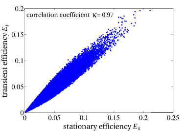
(a) Transport efficiency $E_{t}$ in a transient scenario as a function of the transport efficiency $E_{s}$ in a stationary state.

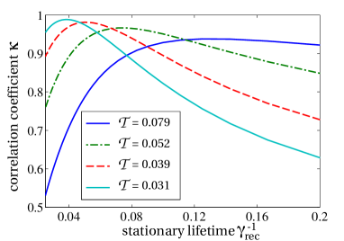
(b) Correlation coefficient $\kappa$ as a function of the stationary state’s excitation lifetime $\gamma_{rec}^{-1}$ for various transient lifetimes $\mathcal{T}$.

Figure 1: Correlation of the stationary transport efficiency $E_{s}$ and its transient analog $E_{t}$ defined in eq. (11) and (7) for the same sample of $10^{5}$ random networks. In the regime of rapid dynamics, i.e. for excitation lifetimes of $\gamma_{rec}^{-1}=0.05$ and $\mathcal{T}=0.039$, subfigure (a) depicts a strong correlation with a coefficient of $\kappa=0.97$. This correlation between $E_{s}$ and $E_{t}$ decreases for longer lifetimes but a decrease in $\mathcal{T}$ requires a decrease in $\gamma_{rec}^{-1}$ in order to keep the correlation maximal as depicted in subfigure (b) which underlines the compatibility of the two approaches.

Fig. 1(a) depicts $E_{t}$ as a function of $E_{s}$ for $10^{5}$ random systems with $N=7$ sites. A sufficiently small choice of the transient excitation lifetime ${\cal T}=\frac{1}{40}{\cal T}_{direct}=\frac{\pi}{80}$ sets the focus on short-time dynamics, i.e. we only identify those networks as efficient in which the excitation can reach the output significantly faster than allowed by the direct interaction between input and output site that takes place on the timescale ${\cal T}_{direct}=\frac{\pi}{2}$. The excitation lifetime in the stationary state is governed by the inverse of the recombination rate $\gamma_{rec}^{-1}=\frac{1}{20}$. As it can be seen in fig. 1(a), $E_{t}$ and $E_{s}$ are highly correlated, i.e. the efficiency in the transient scenario allows to infer about the efficiency in the stationary case and vice versa. The correlations are not perfect, i.e. $E_{t}$ is not a function of $E_{s}$ alone, but it can be quantified by the correlation coefficient

$$\kappa\left(E_{t},E_{s}\right)=\frac{\left\langle\left(E_{t}-\left\langle E_{t}\right\rangle\right)\left(E_{s}-\left\langle E_{s}\right\rangle\right)\right\rangle}{\sigma_{E_{t}}\sigma_{E_{s}}}$$ (12)

where $\sigma_{X}=\sqrt{\langle X^{2}\rangle-\langle X\rangle^{2}}$ is the standard deviation and $\langle X\rangle$ stands for the average over the ensemble of random networks. A correlation coefficient of $\kappa=\pm 1$ indicates that the value of one quantity determines the value of the other exactly, whereas $\kappa=0$ signifies that the knowledge of one does not provide any information about the other. For the data displayed in fig. 1(a) we obtain a correlation of $\kappa\approx 0.97$, i.e. a close-to-maximal value what substantiates that observations made for the transient approach transfer to the stationary scenario essentially perfectly and vice versa.

One might, however, expect that this compatibility of the two transport scenarios relies on the similarity of the transport timescales, i.e., it does not apply anymore if $\gamma_{rec}\cdot{\cal T}$ differs substantially from unity. To test that, we plot $\kappa$ as a function of the recombination rate’s inverse $\gamma_{rec}^{-1}$ for different choices of ${\cal T}$ in fig. 1(b). The case ${\cal T}=\frac{1}{40}{\cal T}_{direct}$ corresponding to fig. 1(a) is depicted in red and a maximum of the correlations for $\gamma_{rec}\approx 0.05$ is clearly discernible. The maximum, however, is rather broad, and strong correlations with $\kappa>0.9$ are obtained for a wide range of excitation lifetimes in the stationary scenario $0.03\lesssim\gamma^{-1}_{rec}\lesssim 0.1$. That is, the transfer of observations between stationary and transient approach does not require precise knowledge of parameters like the recombination rate, but a rough estimate is sufficient for qualitative assessments.

A variation of the transient lifetime ${\cal T}$ confirms that optimal correlation is, however, obtained if ${\cal T}$ and $\gamma_{rec}^{-1}$ define comparable timescales. Fig. 1(b) depicts that the maximum of $\kappa$ is shifted to larger values of $\gamma_{rec}^{-1}$ as ${\cal T}$ is increased what clearly underlines the correspondence between these two timescales. The correlation, however, gets less significant for longer excitation lifetimes that invoke a consideration of networks with less rapid dynamics. Furthermore, optimal correlations are always obtained for $\gamma_{rec}\cdot{\cal T}<1$, i.e. for the case in which the excitation is given a shorter time window in the transient case to reach the output site than in the stationary state scenario. To appreciate this difference one has to take into account the presence of the sink in the stationary state approach which additionally shortens the excitation lifetime. Whereas in the purely coherent case the excitation loss (and therefore also the finite excitation lifetime) is only determined by the value of ${\cal T}$, the stationary state’s excitation lifetime is affected by both recombination and sink drainage. The choice of the sink rate $\gamma_{out}$ does fundamentally affect the period for which an excitation is able to stay in the network as well as the maximally obtainable transport efficiency. In the transient approach, however, there is no comparable analog to the sink, what makes these two concepts differ systematically.

Despite these differences, the correlations between $E_{t}$ and $E_{s}$ as well as the correspondence of $\gamma_{rec}^{-1}$ and ${\cal T}$ suggest a major agreement of the transient and the stationary state approach. Efficiency does thus not primarily depend on the injection mechanism but is a rather universal feature, i.e. a given spacial arrangement shows a similar transport performance under different feed-in scenarios.

4 Transport efficiency and quantum coherence

For the transient scenario it is widely accepted that quantum coherence is a crucial prerequisite for efficient transport across molecular networks [2, 13, 14]. Given the agreement of the transient and the stationary state scenario in terms of efficiency one might raise the question of whether the similarities go beyond the mere transport performance and also hold for the occurrence and role of coherence, i.e. whether coherence in continuously, incoherently driven networks does play the same crucial role for the transport process as assumed for the transient case.

The role of coherence for excitation transport is readily illustrated by the double-slit experiment in which a coherent superposition of two path-alternatives gives rise to an interference pattern of alternating regions of enhanced and reduced arrival probabilities. Increasing the number of coherent path-alternatives through an increasing number of slits changes the interference pattern such that it increases the contrast, i.e. the differences in arrival probabilities between spots with constructive and spots with destructive interference. Similar consequences also apply to an excitation that can take several path-alternatives in order to propagate from the input to the exit. If two of these path-alternatives are in a coherent superposition such that it features constructive interference for the output site then this yields a high arrival probability at the output which, in turn, results in an enhancement in transport efficiency. In analogy the multi-slit experiment this enhancement can even be higher if there is a constructive interference of not only two but three or more path-alternatives. The more different paths are taken coherently, the more potential benefit this can have for the transport efficiency.

A coherent superposition of different path-alternatives, however, requires a coherent delocalization of the excitation over various sites. The number of sites over which an excitation is coherently delocalized and which we also refer to as the extent of coherent delocalization is strongly correlated to number of paths that are in a coherent superposition and can thus be expected to also correlate to the optimal transport efficiency.

4.1 Characterizing coherence in the stationary state

As discussed before, we can restrict the following discussion to the zero- and one-excitation subspace as due to the choice of coupling constants the state amplitudes with more than one excitation are negligible. Since all terms in the equations of motion that mediate excitation (i.e. the Hamiltonian defined in eq. (1)) conserve the number of excitations, the system ground state does not take part in the actual transport so that we only need to consider that part of the density matrix that describes a single excitation.

The objective is to characterize to what extent the excitation is coherently delocalized [30]. For that purpose, we project the density matrix onto the single-excitation subspace and apply a renormalization such that we obtain

$$\tilde{\varrho}=\frac{P\varrho P}{\tr\varrho P}\ \mbox{ with }\ P=\sum_{i=1}^{N}|i\rangle\langle i|\ ,$$ (13)

where $|i\rangle$ denotes the state of the $i^{th}$ site excited and all other sites in the ground state. Since we expect the benefits and disadvantages of quantum coherence to result from constructive and destructive interference of different path-alternatives across the network which, in turn, requires a coherent delocalization of an excitation, we will characterize quantum coherence in terms of the number of sites over which an excitation is coherently delocalized. An excitation in a pure state is coherently delocalized over $K$ sites if the state vector

$$|\Psi_{KN}\rangle=\sum_{i}\psi_{i}|i\rangle\ ,$$ (14)

contains $K$ finite amplitudes $\psi_{i}$. Because of the coupling to incoherent reservoirs we, however, always face mixed states here for which we have to generalize the concept of $K$-site coherence. The formal generalization is fairly straight forward: a mixed state $\tilde{\varrho}_{KN}$ is considered to feature $K$-site coherence if it can not be described as an ensemble of pure states without at least one state-vector with at least $K$-site coherence, i.e.

$$\tilde{\varrho}_{KN}\neq\sum_{j<K}\sum_{i}p_{ij}|\Psi^{(i)}_{jN}\rangle\langle\Psi^{(i)}_{jN}|\ .$$ (15)

Rigorously identifying $K$-body coherence, on the other hand, is typically rather cumbersome, but given the formal similarity between $K$-site coherence and $K$-body entanglement in the one-excitation subspace [11], efficient practical tools can be imported from entanglement theory [21]. We will employ in the following the functions

$$\tau_{KN}(\tilde{\varrho})=\max_{\{\varphi_{i}\}}b_{KN}\left(|\langle\Phi_{1}|\tilde{\varrho}|\Phi_{2}\rangle|-a_{KN}\sum_{i=1}^{N}\sqrt{\langle\Phi^{(i)}_{1}|\tilde{\varrho}|\Phi^{(i)}_{1}\rangle\langle\Phi^{(i)}_{2}|\tilde{\varrho}|\Phi^{(i)}_{2}\rangle}\right)\ ,$$

with $N$-body product state vectors $|\Phi_{1}\rangle$, $|\Phi_{2}\rangle$, $|\Phi^{(i)}_{1}\rangle$, $|\Phi^{(i)}_{2}\rangle$ defined in terms of pairs of orthogonal states (i.e. $\langle\varphi_{i}|\varphi_{i}^{\perp}\rangle=0$) as

$$\begin{array}[]{rclcrcl}|\Phi_{1}\rangle&=&\bigotimes_{i=1}^{N}|\varphi_{i}\rangle\ ,&&|\Phi^{(i)}_{1}\rangle&=&\bigotimes_{j=1}^{i-1}|\varphi_{i}\rangle\otimes|\varphi_{i}^{\perp}\rangle\bigotimes_{j=i+1}^{N}|\varphi_{i}\rangle\ ,\\ |\Phi_{2}\rangle&=&\bigotimes_{i=1}^{N}|\varphi_{i}^{\perp}\rangle,&\mbox{and}&|\Phi^{(i)}_{2}\rangle&=&\bigotimes_{j=1}^{i-1}|\varphi_{i}^{\perp}\rangle\otimes|\varphi_{i}\rangle\bigotimes_{j=i+1}^{N}|\varphi_{i}^{\perp}\rangle\ .\end{array}$$ (19)

With the prefactor $a_{KN}$ defined as

$$a_{KN}=1/\left(N-K+1\right)\textrm{ for }K\neq 2;\quad a_{KN}=1/N\textrm{ for }K=2$$ (21)

$\tau_{KN}$ is non-positive for all $N$-body quantum states with a single excitation that do not have at least $K$-site quantum coherence. The normalization constant $b_{KN}$ is chosen such that $\tau_{KN}$ adopts the value of unity for the state $|W_{KN}\rangle=\sum_{i=1}^{K}|i\rangle/\sqrt{K}$, i.e. the state of a system with $N$ sites and an excitation that is perfectly coherently delocalized over $K$ sites. Although not strictly necessary for reliable identification of $K$-site coherence, we will always perform a numerical optimization over the state-vectors $|\varphi_{i}\rangle$.

4.2 Coherent excitation transport under incoherent driving

With these tools at hand, we can now strive for the characterization of coherence properties and their examination with respect to the stationary transport efficiencies. That is, we would like to verify if coherent delocalization of the excitation is necessary for fast, efficient transport, or whether the identification of this precondition made in the transient regime [13] is no longer possible due to the permanent de-cohering impact of the coupling to heat baths.

There are two extreme regimes, in which the recombination rate $\gamma_{rec}$ is dominant and negligible respectively as compared to the inter-site coupling strengths. In the former case where there is no path for the excitation to reach the output faster than the limit set by $\gamma_{rec}$ the efficiencies are close to zero. In the latter case where $\gamma_{rec}$ is small compared to the average inter-site coupling the excitation will leave through the sink almost with certainty as the probability of a backflow to the light field is low and all networks will be characterized efficient independently of the question whether transport is coherent or not.

We will therefore focus in the following on the intermediate regime where the value of $\gamma_{rec}$ is of the same order of magnitude as the typical site-site coupling, i.e. large enough to permit the identification of fast transport, but still small enough to enable a significant sink flux. We will investigate the coherence properties of all networks with similar currents, that is we introduce a binning of the $E_{s}$-axis with windows of width $\Delta E_{s}$ centered around $E_{s}$. We then consider the average $K$-site coherence

$$\bar{\tau}_{KN}(E_{s})=\langle\tau_{KN}(\tilde{\varrho})\rangle_{E_{s}(\tilde{\varrho})\in w_{E_{s}}}$$ (22)

with the average taken over all networks with a current within the window $w_{E_{s}}=[{E_{s}}-\frac{\Delta E_{s}}{2},E_{s}+\frac{\Delta E_{s}}{2}]$, and the width

$$\sigma_{KN}(E_{s})=\sqrt{\langle(\tau_{KN}(\tilde{\varrho})-\bar{\tau}_{KN})^{2}\rangle_{E_{s}(\tilde{\varrho})\in w_{E_{s}}}}$$ (23)

of the distribution of $\tau_{KN}$ within a bin.

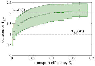
(a) Correlation of two-site coherence $\tau_{2,7}$ and stationary transport efficiency.

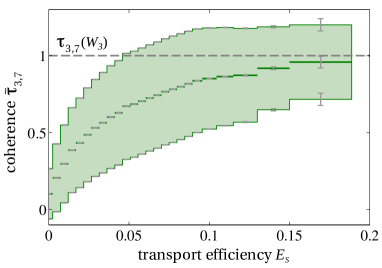
(b) Correlation of three-site coherence $\tau_{3,7}$ and stationary transport efficiency.

Figure 2: Expectation value $\bar{\tau}_{KN}$ (dark green) and standard deviation $\sigma_{KN}$ (light green) of the coherence $\tau_{K,7}$ of $K=2$ (subfigure (a)) and $K=3$ (subfigure (b)) sites as a function of the stationary transport efficiency $E_{s}$ for randomly arranged dephasing-free networks ($\gamma_{deph}=0$). The error bars show the statistical error on the sample mean $\bar{\tau}_{K,7}$ and on the standard deviation $\sigma_{KN}$. The dashed lines represent the coherences $\tau_{K,7}(W_{K^{\prime}})$ for pure $W_{K^{\prime}}$-states and indicate the maximal value of $\tau_{K,7}$ that can be obtained without $(K^{\prime}+1)$-site coherent contribution. Whereas rather strong two-site coherence can be found for almost all systems the most efficient networks excel by a significant extent of three-site coherence.

For the absence of dephasing (i.e. for $\gamma_{deph}=0$) fig. 2(a) and 2(b) depict the average two- and three-site coherence defined in eq. (22) for the recombination rate $\gamma_{rec}=20$. Since this choice of $\gamma_{rec}$ is of the same order of magnitude as the typical interaction strength between two sites, this amounts to rather short-time dynamics. The standard deviation $\sigma_{KN}$ given in eq. (23) is depicted by an bordered area centered around the average value. Additionally to $\sigma_{KN}$ caused by the variance of the coherence properties of different random networks in the same efficiency interval we have to account for a statistical error $S$ on the sample mean $\bar{\tau}_{KN}$ as well as on $\sigma_{KN}$ due to the finite sample size. Such is indicated by error bars and can be estimated by $S(\bar{\tau}_{KN})=\sigma_{KN}/\sqrt{n}$ for the average value and $S(\sigma_{KN})=\Sigma(\sigma_{KN}^{2})/(2\sqrt{\sigma_{KN}})$ for the standard deviation where $n$ is the number of networks per bin and

$$\Sigma^{2}(\sigma_{KN}^{2})=\frac{1}{n}\left(\mu_{4}-\frac{n-3}{n-1}\sigma_{KN}^{4}\right)$$ (24)

is the variance of the sample variance $\sigma_{KN}^{2}$ [31] with $\mu_{4}=\langle(\bar{\tau}_{KN}-\tau_{KN}(\tilde{\varrho}))^{4}\rangle_{E_{s}(\tilde{\varrho})\in\omega_{E_{s}}}$ being the fourth moment about the mean. One finds these statistical errors $S$ to increase for higher efficiencies as efficient networks are less likely to be randomly sampled as compared to rather inefficient configurations [13]. Whereas sample sizes of roughly $2\cdot 10^{3}$ networks per bin are a sound foundation for obtaining reliable expectation values, the bin with the highest efficiency contains less than a hundred networks even though the bin size has been increased.

Despite this statistical error fig. 2 shows a strong correlation between exciton current and coherence, i.e. networks that feature maximal transport also show substantial coherence. Two-site coherence can be detected in almost all networks independently of the excitation flux but gains significance as efficiency increases. As the value of $\tau_{2,7}(W_{2})$ obtained for a pure $W_{2}$-state is significantly exceeded already for fairly low efficiencies (see fig. 2(a)) one can expect a relevant contribution of three-site coherence, which is confirmed by scrutinizing $\bar{\tau}_{3,7}$ in fig. 2(b). The enhancement of efficiency thus requires a substantial extent of coherent delocalization.

In contrast to the case of $\bar{\tau}_{2,7}$, however, significant three-site coherence can not be identified in every network: In the lowest quarter of the efficiency spectrum, i.e. for $E_{s}\leq 0.05$, values of $\bar{\tau}_{3,7}\geq 0.5$ can for example only be found for $46\%$ of all networks. In the most efficient regime $E_{s}\geq 0.15$, this is the case for more than $98\%$ of all systems. This makes three-site coherence a crucial prerequisite for efficient transport.

Coherent delocalization over more than three sites is hardly detectable. As this does not change for larger networks of $N=9$ or $N=12$, we consider this not to be a finite-size effect due to the limited number of sites in the first instance but a consequence of the short time-window provided for establishing coherence which is governed by the maximal excitation lifetime $\gamma_{rec}^{-1}$. Positive values for $\bar{\tau}_{4,7}$ can still be found sporadically but are negligible as compared to $\tau_{4,7}(W_{4})=1$ and the average value $\bar{\tau}_{4,7}$ is smaller than the standard deviation for all efficiencies what prevents any statistical significance. Considering results obtained in a study of the purely coherent transient case [13] we must, however, question whether stronger four-site coherence would indeed yield more efficient transport. While an examination of the coherent case revealed $K$-site coherence with $K=2$ and $K=3$ to be strictly required for high transport efficiency, this relation is weakened drastically for $K\geq 4$. This is reasonable as coherent delocalization as a requirement for constructive interference competes with localization on the output site in order to obtain optimal efficiency. The transport properties for two- and three-site coherent states in the transient scenario do therefore perfectly agree with the results shown here and underline the similarity between coherently and incoherently induced transport.

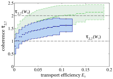
(a) Correlation of two-site coherence $\tau_{2,7}$ and stationary transport efficiency.

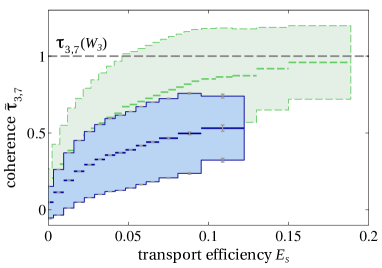
(b) Correlation of three-site coherence $\tau_{3,7}$ and stationary transport efficiency.

Figure 3: Expectation value $\bar{\tau}_{KN}$ (dark blue) and standard deviation $\sigma_{KN}$ (light blue) of the coherence $\tau_{K,7}$ of $K=2$ (subfigure (a)) and $K=3$ (subfigure (b)) sites as a function of the stationary transport efficiency $E_{s}$ for randomly arranged networks exposed to a dephasing of $\gamma_{deph}=10$. The error bars show the statistical error on the sample mean $\bar{\tau}_{K,7}$ and on the standard deviation $\sigma_{KN}$. Comparing the results with the dephasing-free scenario depicted in fig. 2 (shown here dashed and in green) one finds the correlation between coherence and efficiency to be robust under dephasing. Despite the decrease in efficiency of formerly optimal networks the most efficient systems still employ a significant extent of coherence which thus can be deemed required for high efficiencies.

Despite the dephasing impact of the reservoirs and the recombination, networks of suitable geometry have been shown to induce a sufficient amount of coherence which has been identified as a prerequisite for optimal transport. To test if the correlation between coherence and efficiency persists under the application of additional dephasing, we modify the situation discussed before by changing the dephasing rate to $\gamma_{deph}=10$. The coherence time $\gamma_{deph}^{-1}=0.1$ is now comparable to the excitation lifetime $\gamma_{rec}^{-1}=0.05$ that defines the time window relevant for the system dynamics. This situation thus corresponds to the case of real-world light-harvesting complexes where the coherence time has been determined experimentally to be of the same order as the transport time [2, 3]. A comparison of the transport and coherence properties in the dephasing-free approach depicted in fig. 2 and the case of additional dephasing assumed for fig. 3 suggests that the incorporation of additional noise does not qualitatively change the relation between coherence and transport efficiency. Whereas a finite value of $\gamma_{deph}$ leads to reduced coherence the correlation between $\bar{\tau}_{K,7}$ and transport efficiency stays rather unaffected. This is in perfect agreement with the decrease of the maximal efficiency when comparing fig. 2(a) to fig. 2(b), which shows that optimal networks loose efficiency when they are exposed to dephasing. Despite the additional noise suitable systems are, however, capable to successfully employ interference as long as the system can accumulate a sufficient amount of coherence.

5 Conclusion

Based on a comparison of transport efficiencies we found strong similarities between the coherently induced transient and the incoherently induced stationary excitation transport suggesting that the underlying transport mechanisms of these two scenarios are rather similar. It is this similarity which raises the question if long-lived quantum coherence that has been experimentally identified in the transient picture [2, 3, 4, 5, 8] is also relevant for the stationary state approach or whether this analogy does not apply due to the incoherent nature of the light source in the latter case [16, 17, 18].

An application of recent tools from entanglement theory [21] on incoherently driven random networks reveals a strong correlation between coherence and transport efficiency and provides a clear interpretation of the considered concept of coherence which in our context always refers to a coherent delocalization of an excitation over various pigments. This suggests in particular that suitable molecular networks are capable to exploit quantum coherent delocalization of excitations for the purpose of efficient excitation transport even if they are driven by a thermal light source as the sun. Comparing these outcomes to results obtained for the completely coherent and transient transport scenario [13] this permits the conclusion that observations and concepts made for the transient scenario can at least qualitatively be transferred to the stationary case and vice versa [7]. The coherent beatings detected in two-dimensional spectroscopy experiments can therefore be considered as evidence of coherence also in the case of continuous incoherent driving [19, 20, 7].

Our results are robust under the application of additional dephasing, i.e. under the decrease of coherence time. Whereas the latter hinders transport for networks that have originally achieved optimal efficiency, it does not qualitatively affect the correlation between coherent delocalization and stationary transport efficiency. Consequently, networks of suitable geometry are capable to employ quantum coherence in order to obtain optimal transport as long as they can induce a sufficient amount of coherence, i.e. as long as the coherence time is comparable to the transport time. That is, if a system’s protection against decoherence is good enough to preserve quantum coherence on the timescale of the excitation transfer, then this coherence can contribute to an enhanced transport efficiency. Based on the observations done in two-dimensional spectroscopy experiments this is the case for various biological light-harvesting complexes at physiological temperature [3] such that our results can be taken as a strong argument for nature to employ quantum coherence for transport efficiency enhancement.

References

References

- [1] Chain R K and Arnon D I 1977 Proc. Natl Acad. Sci. USA 74 3377–81
- [2] Engel G S, Calhoun T R, Read E L, Ahn T K, Mančal T, Cheng Y C, Blankenship R E and Fleming G R 2007 Nature 446 782–6
- [3] Panitchayangkoon G, Hayes D, Fransted K A, Caram J R, Harel E, Wen J, Blankenship R E and Engel G S 2010 Proc. Natl Acad. Sci. USA 107 12766–70
- [4] Calhoun T R, Ginsberg N S, Schlau-Cohen G S, Cheng Y C, Ballottari M, Bassi R and Fleming G R 2009 J. Phys. Chem. B 113 16291–5
- [5] Schlau-Cohen G S, Calhoun T R, Ginsberg N S, Read E L, Ballottari M, Bassi R, van Grondelle R and Fleming G R 2009 J. Phys. Chem. B 113 15352–63
- [6] Manzano D 2013 PLoS ONE 8 e57041
- [7] Jesenko S 2013 arXiv:1303.2046v2
- [8] Collini E, Wong C Y, Wilk K E, Curmi P M G, Brumer P and Scholes G D 2010 Nature 463 644–7
- [9] Wilde M M, McCracken J M and Mizel A 2009 Proc. R. Soc. A 466 1347–63
- [10] Tiersch M, Popescu S and Briegel H J 2012 Phil. Trans. R. Soc. A 370 3771–86
- [11] Ishizaki A and Fleming G R 2010 New. J. Phys. 12 055004
- [12] Scholes G D, Fleming G R, Olaya-Castro A and van Grondelle R 2011 Nat. Chem. 3 763–74
- [13] Scholak T, de Melo F, Wellens T, Mintert F and Buchleitner A 2011 Phys. Rev. E 83 021912
- [14] Zech T, Mulet R, Wellens T and Buchleitner A 2012 arXiv:1205.5519v1
- [15] Ishizaki A and Fleming G R 2009 Proceedings of the National Academy of Sciences of the USA 106 17255–60
- [16] Brumer P and Shapiro M 2012 Proc. Natl Acad. Sci. USA 109 19575–8
- [17] Mančal T and Valkunas L 2010 New. J. Phys. 12 065044
- [18] Pachón L A and Brumer P 2013 Phys. Rev. A 87 022106
- [19] Fassioli F, Olaya-Castro A and Scholes G D 2012 J. Phys. Chem. Lett. 3 3136–3142
- [20] Kassal I, Yuen-Zhou J and Rahimi-Keshari S 2013 J. Phys. Chem. Lett. 4 362–367
- [21] Levi F and Mintert F 2013 Phys. Rev. Lett. 110 150402
- [22] Adolphs J and Renger T 2006 Biophys. J. 91 2778–97
- [23] Breuer H P and Petruccione F 2002 The Theory of Open Quantum Systems (Oxford University Press)
- [24] Rebentrost P, Mohseni M and Aspuru-Guzik A 2009 J. Phys. Chem. B 113 9942–7
- [25] Mohseni M, Rebentrost P, Lloyd S and Aspuru-Guzik A 2008 J. Chem. Phys. 129 174106
- [26] Rebentrost P, Mohseni M, Kassal I, Lloyd S and Aspuru-Guzik A 2009 New. J. Phys. 11 033003
- [27] Owens T G, Webb S P, Mets L, Alberte R S and Fleming G R 1987 Proc. Natl Acad. Sci. USA 84 1532–6
- [28] Fassioli F, Olaya-Castro A, Scheuring S, Sturgis J N and Johnson N F 2009 Biophys. J. 97 2464–73
- [29] Manzano D, Tiersch M, Asadian A and Briegel H J 2012 Phys. Rev. E 86 061118
- [30] Smyth C, Fassioli F and Scholes G D 2012 Phil. Trans. R. Soc. A 370 3728–49
- [31] Neter J, Wasserman W and Kutner M H 1990 Applied Linear Statistical Models (CRC Press)