Open Shell Effects in a Microscopic Optical Potential for Elastic Scattering of ⁶⁽⁸⁾He

Abstract

Elastic scattering observables (differential cross section and analyzing power) are calculated for the reaction ⁶He(p,p)⁶He at projectile energies starting at 71 MeV/nucleon. The optical potential needed to describe the reaction is based on a microscopic Watson first-order folding potential, which explicitly takes into account that the two neutrons outside the ⁴He-core occupy an open p-shell. The folding of the single-particle harmonic oscillator density matrix with the nucleon-nucleon t-matrix leads for this case to new terms not present in traditional folding optical potentials for closed shell nuclei. The effect of those new terms on the elastic scattering observables is investigated. Furthermore, the influence of an exponential tail of the p-shell wave functions on the scattering observables is studied, as well as the sensitivity of the observables to variations of matter and charge radius. Finally elastic scattering observables for the reaction ⁸He(p,p)⁸He are presented at selected projectile energies.

I Introduction

The exotic helium isotopes have been extensively studied, both experimentally and theoretically. The charge radii of ⁶He and ⁸He are experimentally very well known Wang et al. (2004); Mueller et al. (2007); Brodeur et al. (2012). The nucleus ⁶He is of particular interest since it constitutes the lightest two-neutron halo nucleus with a ⁴He core. Investigating its structure already inspired a large body of work including effective few-body models Lehman and Parke (1983); Zhukov et al. (1993); Fedorov et al. (2003), multi-cluster methods Csoto (1993); Varga et al. (1994); Wurzer and Hofmann (1997) Green’s Function Monte Carlo (GFMC) methods Pudliner et al. (1997), and no-core shell model calculations Navratil (2004); Navratil et al. (2009); Bacca et al. (2012), so that ground state properties of ⁶He appear to be quite well understood. Similarly, the ground state properties of ⁸He have been explored with different theoretical methods Bacca et al. (2009); Itagaki et al. (2008).

Recently, elastic scattering of ⁶He Uesaka et al. (2010); Hatano et al. (2005) as well as ⁸He Sakaguchi et al. (2013) off a polarized proton target has been measured for the first time at a laboratory kinetic energy of 71 MeV/nucleon. The experiments find that for ⁶He the analyzing power $A_{y}$ becomes negative around 50^o, whereas for ⁸He it stays positive. Specifically the behavior of $A_{y}$ for ⁶He not predicted by simple folding models for the optical potentials Weppner et al. (2000); Gupta et al. (2000), though the calculations reproduce the differential cross section at this energy reasonably well.

This apparent “$A_{y}$ problem” conveys the inadequacy of using the same methods which describe p-A scattering from stable nuclei for reactions involving halo nuclei. The obvious difference is the nuclear structure. Traditionally, microscopic folding models are developed for closed shell nuclei, like ¹⁶O, ⁴⁰Ca, or ²⁰⁸Pb. Though ⁶He and ⁸He are both spin-0 nuclei, their outer p-shell is not fully occupied. In the case of ⁶He two neutrons occupy the p-shell. This structure suggests describing ⁶He with three-body cluster models, as pioneered in Refs. Crespo et al. (2006); Crespo and Moro (2007) for higher energies. For describing the differential cross section and the analyzing power at 71 MeV/nucleon, Refs. Uesaka et al. (2010); Weppner and Elster (2012) use “cluster-folding” calculations with still only limited success at understanding the $A_{y}$ problem.

The focus of this work is to extend traditional microscopic folding models to take the valence neutrons in ⁶⁽⁸⁾He explicitly into account. In order to facilitate this calculation, we assume a simple harmonic oscillator model ansatz for ⁶⁽⁸⁾He. In Section II we derive the formulation for a microscopic optical potential which takes into account the partially occupied p-shell of ⁶He, and show the resulting effect on the differential cross section and the analyzing power at different energies. Since we use a model based on oscillator wave functions, we investigate in Section III, if this specific functional form of the wave functions has an effect on the scattering observables at energies of 71 MeV/nucleon and higher. Specifically we study, if there is a difference at these energies between wave functions that fall off exponentially in coordinate space or harmonic oscillator wave functions. In Section IV we study the sensitivity of the scattering observables to the charge and matter radii of ⁶He. In Section V we study the open shell effects in the optical potential on the scattering observables for ⁸He. We conclude in Section VI.

II Open Shell Effects in the Optical Potential for ⁶He

Let $H=H_{0}+V$ be the Hamiltonian for the nucleon-nucleus system in which the interaction $V=\sum_{i=1}^{A}v_{0i}$ consists of all two-nucleon interactions $v_{0i}$ between the projectile (“$0$”) and a target nucleon (“$i$”). The free Hamiltonian is given by $H_{0}=h_{0}+H_{A}$, where $h_{0}$ describes the kinetic energy of the projectile, while the target Hamiltonian $H_{A}$ satisfies $H_{A}|\Phi_{A}\rangle=E_{A}|\Phi_{A}\rangle$, with $|\Phi_{A}\rangle$ being the ground state of the target. Focusing on elastic scattering, the transition operator is given by

$$PTP\equiv T_{el}=PUP+PUPG_{0}(E)PT_{el},$$ (1)

where $P=\frac{|\Phi_{A}\rangle\langle\Phi_{A}|}{\langle\Phi_{A}|\Phi_{A}\rangle}$ is the projection operator onto the ground state $|\Phi_{A}\rangle$ with $P+Q={\bf 1}$, where $Q$ projects onto the orthogonal space, and $G_{0}(E)=(E-h_{0}-H_{A}+i\varepsilon)^{-1}$ is the propagator, which here will be treated in impulse approximation. The Watson first-order optical potential operator for scattering of protons is given by Chinn et al. (1993) and Appendix A of Ref. Weppner and Elster (2012)

$$U_{p}=\sum_{i=1}^{Z}\tau_{0i}^{pp}+\sum_{i=1}^{N}\tau_{0i}^{np}\equiv U_{p}^{Z}+U_{p}^{N},$$ (2)

where the two-body transition operators $\tau^{pp(np)}_{0i}$ are related to the proton-proton ($pp$) and neutron-proton ($np$) t-matrices $\hat{\tau}^{pp(np)}_{0i}$ via Chinn et al. (1993)

$$\tau^{pp(np)}_{0i}={\hat{\tau}}^{pp(np)}_{0i}-{\hat{\tau}^{pp(np)}_{0i}}G_{0}(E)P\tau^{pp(np)}_{0i}.$$ (3)

As function of the external momenta ${\bf{k}}$ and ${\bf{k}}^{\prime}$ the first-order optical potential is given by

$$\langle{\bf{k}}^{\prime}|\langle\phi_{A}|PUP|\phi_{A}\rangle|{\bf{k}}\rangle\equiv U_{el}({\bf{k}}^{\prime},{\bf{k}})=\sum_{i=N,P}\left\langle{\bf{k}}^{\prime}|\langle\phi_{A}|\hat{\tau}_{0i}({\cal{E}})|\phi_{A}\rangle|{\bf{k}}\right\rangle,$$ (4)

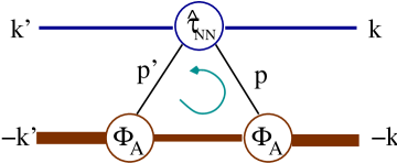
Figure 1: Diagram for the folding optical potential matrix element in the single-scattering approximation.

where ${\cal{E}}$ is the energy of the system. In this work the common approximation of fixing ${\cal{E}}$ at half the laboratory energy will be used. The summation over $i$ indicates that one has to sum over $N$ neutrons and $Z$ protons. The structure of Eq. (4) is schematically indicated in Fig. 1, where ${\bf{p}}$ and ${\bf{p}}^{\prime}$ are the internal variables of the struck target nucleon, which enter into the two-body t-matrices as well as the single-particle densities.

Let us first consider the nucleon-nucleon (NN) t-matrix. On the energy shell, the NN scattering-amplitude matrix $\overline{M}({\bf{p}}^{\prime}_{NN},{\bf{p}}_{NN})$ is related to the on-shell transition matrix element as $\overline{M}({\bf{p}}^{\prime}_{NN},{\bf{p}}_{NN})=-4\pi^{2}\mu_{NN}\langle{\bf{p}}^{\prime}_{NN}|\hat{\tau}_{0i}|{\bf{p}}_{NN}\rangle$, where $\mu_{NN}$ is the reduced mass of the two-nucleon system. The off-shell Wolfenstein Wolfenstein and Ashkin (1952) parameterization of $\overline{M}({\bf{p}}^{\prime}_{NN},{\bf{p}}_{NN})$ is given by

$$\overline{M} = AI+iC(\mbox{\boldmath$\sigma$}^{(0)}\otimes I+I\otimes\mbox{\boldmath$\sigma$}^{(i)})\cdot\hat{\mathbf{n}}_{NN}+M(\mbox{\boldmath$\sigma$}^{(0)}\cdot\hat{\mathbf{n}}_{NN})\otimes(\mbox{\boldmath$\sigma$}^{(i)}\cdot\hat{\mathbf{n}}_{NN})$$ (7)

$$+(G+H)(\mbox{\boldmath$\sigma$}^{(0)}\cdot\hat{\mathbf{K}}_{NN})\otimes(\mbox{\boldmath$\sigma$}^{(i)}\cdot\hat{\mathbf{K}}_{NN})+(G-H)(\mbox{\boldmath$\sigma$}^{(0)}\cdot\hat{\mathbf{q}}_{NN})\otimes(\mbox{\boldmath$\sigma$}^{(i)}\cdot\hat{\mathbf{q}}_{NN})$$

$$+D\left((\mbox{\boldmath$\sigma$}^{(0)}\cdot\hat{\mathbf{q}}_{NN})\otimes(\mbox{\boldmath$\sigma$}^{(i)}\cdot\hat{\mathbf{K}}_{NN})+(\sigma^{(0)}\cdot\hat{\mathbf{K}}_{NN})\otimes(\mbox{\boldmath$\sigma$}^{(i)}\cdot\hat{\mathbf{q}}_{NN})\right)$$

The spin-momentum operators of Eq. (7) are invariant with respect to rotations, and spin exchange. They are time reversal invariant with the exception of the last operator, which changes sign and thus is paired with a coefficient function $D$, that is odd in $|{\bf{p}}^{\prime}_{NN}|^{2}-|{\bf{p}}_{NN}|^{2}$, and thus vanishes on-shell. The Wolfenstein amplitudes are functions of the vector variables ${\bf{p}}^{\prime}_{NN}$ and ${\bf{p}}_{NN}$ and can be either calculated directly as such Veerasamy et al. (2012) or obtained from partial wave sums. The momentum vectors are defined as ${\bf{q}}_{NN}={\bf{p}}^{\prime}_{NN}-{\bf{p}}_{NN}$, ${\bf{K}}_{NN}={\bf{p}}^{\prime}_{NN}+{\bf{p}}_{NN}$, and ${\bf{n}}_{NN}={\bf{p}}^{\prime}_{NN}\times{\bf{p}}_{NN}$, and given in the two-nucleon intrinsic frame.

For the calculation of the optical potential of Eq. (4) the expectation values of these spin-momentum operators need to be calculated in the plane-wave basis for the projectile characterized by $\mbox{\boldmath$\sigma$}^{(0)}$ and in a nuclear basis for the struck nucleon characterized by $\mbox{\boldmath$\sigma$}^{(i)}$.

II.1 Model for the Single Particle Density of ⁶He

Since our goal is to explore the folding optical potential for a nucleus with an open-shell structure, we first need to consider the explicit angular momentum and spin structure of the single particle density that enters the folding optical potential. Without loss of generality we assume nucleon “$1$” is the struck target nucleon, so that

$$\rho_{I,M_{I};I,M_{I}}(1,1^{\prime}) = \int\prod_{l=2}^{A-1}d{\bf\zeta_{l}^{\prime}}\int\prod_{j=2}^{A-1}d{\bf\zeta_{j}}\langle\phi_{I,M_{I}}|{\bf{\zeta}}_{1}^{\prime}{\bf{\zeta}}_{2}^{\prime}{\bf{\zeta}}_{3}^{\prime}{\bf{\zeta}}_{4}^{\prime}...{\bf{\zeta}}_{A-1}^{\prime}\rangle\;\langle{\bf{\zeta}}_{1}{\bf{\zeta}}_{2}{\bf{\zeta}}_{3}{\bf{\zeta}}_{4}...{\bf{\zeta}}_{A-1}|\phi_{I,M_{I}^{\prime}}\rangle$$ (8)

$$\equiv \langle\phi_{I,M_{I}}|\psi^{\dagger}(1)\psi(1^{\prime})|\phi_{I,M_{I}}\rangle,$$ (9)

where $I$ is the total angular momentum of the ground state, and $M_{I}$ its projection. All internal variables integrate out, and one is left with an operator $\psi^{\dagger}(1)$ that creates a nucleon with given quantum numbers “$1$”, e.g. momentum and spin, which can then be expanded in terms of single particle wave functions $\phi_{nljm}(1)$ as

$$\psi^{\dagger}(1)=\sum_{nljm}\phi_{nljm}(1)(a_{nljm})^{\dagger}.$$ (10)

Expanding the single particle wave function explicitly into spin, orbital angular momentum, and radial parts leads to

$$\rho_{I,M_{I};I,M^{\prime}_{I}}(1,1^{\prime}) = \sum C_{\lambda\hskip 1.0ptm_{s}\hskip 1.0ptm}^{l\hskip 3.0pt\frac{1}{2}\hskip 6.0ptj}C_{\lambda^{\prime}\hskip 2.0ptm^{\prime}_{s}\hskip 1.0ptm^{\prime}}^{l^{\prime}\hskip 3.0pt\frac{1}{2}\hskip 6.0ptj^{\prime}}\;Y_{l}^{\lambda}(1)\chi_{m_{s}}(1)R_{nlj}(1)\;Y_{l^{\prime}}^{*\lambda^{\prime}}(1^{\prime})\chi^{*}_{m^{\prime}_{s}}(1^{\prime})R^{*}_{n^{\prime}l^{\prime}j^{\prime}}(1^{\prime})$$ (12)

$$\times\langle\phi_{I,M_{I}}|(a_{nljm})^{\dagger}a_{n^{\prime}l^{\prime}j^{\prime}m^{\prime}}|\phi_{I,M^{\prime}_{I}}\rangle.$$

Here the sum is taken over all quantum numbers occurring in the sum. This expression exhibits the spin eigenfunctions of the struck nucleon, but is not yet in a form best suited for evaluation of matrix elements. Let us define a tensor operator $\tau_{k_{s},q_{s}}(s=\frac{1}{2})$ for which $k_{s}$ =0 or 1 with

$$\tau_{00} = 1$$ (13)

$$\tau_{10} = 2\sigma_{z}$$ (14)

$$\tau_{1\pm 1} = \frac{1}{\sqrt{2}}{\mp}(\sigma_{x}\pm i\sigma_{y}),$$ (15)

where $\sigma_{i}$ are the usual spin-projections. The matrix elements of this operator can be written as

$$\langle sm_{s}|\tau_{k_{s},q_{s}}(s)|sm^{\prime}_{s}\rangle=\sqrt{2k_{s}+1}\;C_{m^{\prime}_{s}\hskip 1.0ptq_{s}\hskip 1.0ptm_{s}}^{s\hskip 5.0ptk_{s}\hskip 4.0pts}$$ (16)

Inserting Eq. (16) into Eq. (12) and re-coupling the angular momenta leads to

$$\rho_{I,M_{I};I,M_{I}}(1,1^{\prime}) = \sum_{k_{l},q_{l},k_{s},q_{s},k,q,\cdots}{\mathcal{N}}\langle\phi_{I,M_{I}}|(a_{nljm})^{\dagger}a_{n^{\prime}l^{\prime}j^{\prime}m^{\prime}}|\phi_{I,M^{\prime}_{I}}\rangle$$ (22)

$$(-1)^{j^{\prime}-m^{\prime}}\;C_{m\hskip 1.0pt-m^{\prime}\hskip 1.0ptq}^{j\hskip 6.0ptj^{\prime}\hskip 6.0ptk}\;\;(-1)^{l^{\prime}-\lambda^{\prime}}\;C_{\lambda\hskip 1.0pt-\lambda^{\prime}\hskip 1.0ptq_{l}}^{l\hskip 6.0ptl^{\prime}\hskip 6.0ptk_{l}}\;\;C_{q_{l}\hskip 1.0ptq_{s}\hskip 1.0ptq}^{k_{l}\hskip 1.0ptk_{s}\hskip 1.0ptk}\left\{\begin{array}[]{ccc}~{}l~{}~{}l^{\prime}~{}~{}k_{l}{}\\ ~{}s~{}~{}s~{}~{}k_{s}{}\\ ~{}j~{}~{}j^{\prime}~{}~{}k{}\end{array}\right\}$$

$$\times Y_{l}^{\lambda}(1)\;R_{nlj}(1)\;Y_{l^{\prime}}^{*\lambda^{\prime}}(1^{\prime})\;R^{*}_{n^{\prime}l^{\prime}j^{\prime}}(1^{\prime}),$$

where all constants are collected in the number ${\mathcal{N}}$ and only the newly introduced quantum numbers are shown in the sum. From this expression, the terms related to the orbital angular momentum can be extracted as

$${\mathcal{L}}^{ll^{\prime}}_{k_{l}q_{l}}(1,1^{\prime})\equiv\sum_{ll^{\prime}}(-1)^{l^{\prime}-\lambda^{\prime}}\;C_{\lambda\hskip 1.0pt-\lambda^{\prime}\hskip 1.0ptq_{l}}^{l\hskip 6.0ptl^{\prime}\hskip 6.0ptk_{l}}\;Y_{l}^{\lambda}(1)\;\;Y_{l^{\prime}}^{*\lambda^{\prime}}(1^{\prime}).$$ (23)

For evaluating the matrix element $\langle\phi_{I,M_{I}}|(a_{nljm})^{\dagger}a_{n^{\prime}l^{\prime}j^{\prime}m^{\prime}}|\phi_{I,M^{\prime}_{I}}\rangle$ let us consider

$${\mathcal{Q}}_{k,q} \equiv \left\langle\phi_{I,M_{I}}\left|\sum_{mm^{\prime}}(-1)^{j^{\prime}-m^{\prime}}C_{m\hskip 1.0pt-m^{\prime}\hskip 1.0ptq}^{j\hskip 6.0ptj^{\prime}\hskip 6.0ptk}(a_{nljm})^{\dagger}a_{n^{\prime}l^{\prime}j^{\prime}m^{\prime}}\right|\phi_{I,M^{\prime}_{I}}\right\rangle$$ (24)

$$= C_{M^{\prime}_{I}\hskip 1.0ptq\hskip 1.0ptM_{I}}^{I\hskip 6.0ptk\hskip 6.0ptI}\;\langle\phi_{I,M_{I}}||\rho_{k}(nlj;n^{\prime}l^{\prime}j)||\phi_{I,M^{\prime}_{I}}\rangle,$$ (25)

where the reduced matrix element consists of complex numbers and is independent of $M_{I}$, $q$, and $M^{\prime}_{I}$.

Thus, the angular momentum and spin structure of the single particle density matrix is schematically given as

$$\rho_{I,M_{I};I,M^{\prime}_{I}}(1,1^{\prime}) \simeq \sum_{k_{l},q_{l},k_{s},q_{s},k,q,\cdots}{\mathcal{N}}\;{\mathcal{Q}}_{q,k}\;{\mathcal{L}}^{ll^{\prime}}_{k_{l}q_{l}}(1,1^{\prime})\;R_{nlj}(1)\;R^{*}_{n^{\prime}l^{\prime}j^{\prime}}(1^{\prime})$$ (30)

$$\langle sm_{s}|\tau_{k_{s}q_{s}}(s)|sm^{\prime}_{s}\rangle\;C_{q_{l}\hskip 1.0ptq_{s}\hskip 1.0ptq}^{k_{l}\hskip 1.0ptk_{s}\hskip 1.0ptk}\left\{\begin{array}[]{ccc}~{}l~{}~{}l^{\prime}~{}~{}k_{l}{}\\ ~{}s~{}~{}s~{}~{}k_{s}{}\\ ~{}j~{}~{}j^{\prime}~{}~{}k{}\end{array}\right\}.$$

For a spin-zero target, $I=M_{I}=M^{\prime}_{I}=0$, the Clebsch-Gordan coefficient in Eq. (25) requires $k=q=0$. Consequently, the Clebsch-Gordan coefficient of Eq. (30) requires $k_{s}=k_{l}$. Thus, for $l=0$ only $k_{s}=0$ is possible, i.e. the s-shell can not have any spin-dependent contribution.

For the consideration of ⁶He we make the assumption of an occupied s-shell, the alpha core, and the valence neutrons occupying the p-shell. We approximate the density matrix by two harmonic oscillator terms. The one-particle s-wave harmonic oscillator wave function is given by

$$\Phi^{m}_{s}({\bf{p}})=\left(\frac{4}{\sqrt{\pi\nu_{s}^{3}}}\right)^{1/2}e^{-p^{2}/2\nu_{s}}\;{\cal Y}_{0}^{\frac{1}{2},m}({\hat{{\bf{p}}}})\equiv f_{s}(p)\;{\cal Y}_{0}^{\frac{1}{2},m}({\hat{{\bf{p}}}}),$$ (31)

and the one-particle p-wave harmonic oscillator wave function by

$$\Phi^{m}_{p}({\bf{p}})=\left(\frac{8}{3\sqrt{\pi\nu_{p}^{5}}}\right)^{1/2}\;p\;e^{-p^{2}/2\nu_{p}}\;{\cal Y}_{1}^{\frac{3}{2},m}({\hat{{\bf{p}}}})\equiv f_{p}(p)\;{\cal Y}_{1}^{\frac{3}{2},m}({\hat{{\bf{p}}}}).$$ (32)

Both wave functions are normalized to one. The functions ${\cal Y}_{l}^{j=l\pm\frac{1}{2},m}({\hat{\bf p}})$ represent the total angular momentum wave functions. The alpha-core consists of a filled s-shell contribution for protons as well as neutrons. According to Eq. (30) the s-wave single-particle density matrix is a scalar function given by

$$\rho_{s}({\bf{p}},{\bf{p}}^{\prime})=\Phi_{s}^{*}({\bf{p}})\Phi_{s}({\bf{p}}^{\prime})=\left(\frac{1}{\pi\nu_{s}}\right)^{\frac{3}{2}}e^{-\frac{p^{2}+p^{\prime 2}}{2\nu_{s}}},$$ (33)

where the sum over $m$ has been carried out.

For the p-shell we make the assumption that the valence neutrons occupy the lowest possible state, the $p_{3/2}$-shell. According to Eq. (30), $k_{l}=1$, and both, $k_{s}=0$ and $k_{s}=1$ are possible. Evaluating the $k_{s}=0$ part for $l=l^{\prime}=1$ according to Eq. (30) leads to

$$\rho_{p}({\bf{p}},{\bf{p}}^{\prime})=\frac{2}{3}\left(\frac{1}{\pi^{3}\nu_{p}^{5}}\right)^{\frac{1}{2}}{\bf{p}}\cdot{\bf{p}}^{\prime}\;e^{-\frac{p^{\prime 2}+p^{2}}{2\nu_{p}}}.$$ (34)

The contribution according to $k_{s}=1$ leads to a spin-dependent piece, which will enter in the explicit calculation of the expectation values of spin-momentum operators in Section II.2 and Appendix A.

Changing variables in Eq. (34) to

$${\bf{q}} = \frac{A}{A-1}({\bf{p}}-{\bf{p}}^{\prime})$$ (35)

$${\bf{P}} = \frac{1}{2}({\bf{p}}+{\bf{p}}^{\prime})$$ (36)

results in

$${\bf{p}}\cdot{\bf{p}}^{\prime} = P^{2}-\left(\frac{A-1}{2A}\right)^{2}q^{2}$$ (37)

$$p^{2}+p^{\prime 2} = 2P^{2}+2\left(\frac{A-1}{2A}\right)^{2}q^{2}.$$ (38)

With these variables the single-particle density matrices of Eqs. (33) and (34) become

$$\rho_{s}({\bf{q}},{\bf{P}}) = \left(\frac{1}{\pi\nu_{s}}\right)^{\frac{3}{2}}e^{-\frac{1}{\nu_{s}}\left({P^{2}}+\left(\frac{A-1}{2A}\right)^{2}q^{2}\right)}$$ (39)

$$\rho_{p}({\bf{q}},{\bf{P}}) = \frac{2}{3}\left(\frac{1}{\pi^{3}\nu^{5}}\right)^{\frac{1}{2}}\left(P^{2}-\left(\frac{A-1}{2A}\right)^{2}q^{2}\right)e^{-\frac{1}{\nu_{p}}\left(P^{2}+\left(\frac{A-1}{2A}\right)^{2}q^{2}\right)}.$$ (40)

From this we obtain the spin-independent single-particle density matrix of ⁶He as

$$\rho_{{}^{6}\rm{He}}({\bf{q}},{\bf{P}})=4\rho_{s}({\bf{q}},{\bf{P}})+2\rho_{p}({\bf{q}},{\bf{P}}).$$ (41)

Integrating over the momentum ${\bf{P}}$ leads to the diagonal density

$$\rho_{{}^{6}\rm{He}}({\bf{q}})=4e^{-\left(\frac{A-1}{2A}\right)^{2}\>\frac{q^{2}}{\nu_{s}}}+2\left(1-\frac{q^{2}}{6\nu_{p}}\right)\;e^{-\left(\frac{A-1}{2A}\right)^{2}\>\frac{q^{2}}{\nu_{p}}}.$$ (42)

It remains to determine the oscillator parameters for the two helium isotopes. The charge radii for ⁶He Mueller et al. (2007) and ⁸He Brodeur et al. (2012) are very well measured, and are used to determine the oscillator parameters for the s-shell according to

$$\langle r^{2}_{ch}\rangle=\frac{3}{2\nu_{s}}.$$ (43)

The matter radius is determined by taking the expectation value of the radius with the total wave function. Using the prior determined s-shell oscillator parameter we obtain the matter radius of ⁶He by

$$\langle r^{2}_{mat}\rangle=\frac{1}{6}\left(\frac{5}{\nu_{p}}+\frac{6}{\nu_{s}}\right)$$ (44)

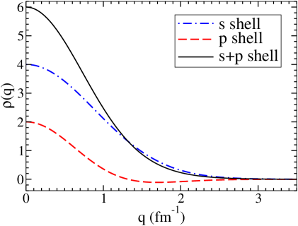
Figure 2: (Color online) The diagonal density of ⁶He normalized to the total particle number. The s-shell (dashed) and p-shell (dash-dotted) are given separately.

and from this the value for $\nu_{p}$. The experimental extractions of the matter radii used for our calculations are given in Table 1. The so obtained diagonal density for ⁶He is shown in Fig. 2 as function of the momentum transfer. The density is normalized such $\rho_{{}^{6}\rm{He}}(0)=6$.

II.2 Expectation Values of the Spin-Momentum Operators for the Target Nucleon

Having established a basis for the nuclear single-particle density matrix allows the calculation of the matrix elements of the optical potential given in Eq. (4). When considering the first Wolfenstein amplitude in Eq. (7), we encounter the unit matrix between the plane wave and the nuclear basis states. This leads after a series of variable transformations, which are in detail given in Ref. Weppner and Elster (2012), to the central part of the optical potential

$$U_{A}({\bf{q}},{\bf{K}}) = \int d^{3}P\;A\left({\bf{q}},\frac{1}{2}\left(\frac{A+1}{A}{\bf{K}}-{\bf{P}}\right),{\cal{E}}\right)\rho_{i}\left({\bf{P}}-\frac{A-1}{2A}{\bf{q}},{\bf{P}}+\frac{A-1}{2A}{\bf{q}}\right)$$ (45)

$$= \int d^{3}P\;A\left({\bf{q}},\frac{1}{2}\left(\frac{A+1}{A}{\bf{K}}-{\bf{P}}\right),{\cal{E}}\right)\rho_{s(p)}({\bf{q}},{\bf{P}}),$$ (46)

where ${\bf{q}}$ is the momentum transfer, ${\bf{K}}$ the momentum orthogonal to it, and ${\bf{P}}$ the total momentum of the struck nucleon. The second line contains the explicit expressions for the single-particle densities of Eq. (40) and should be read as the sum over the s- and p-shell contributions.

The next term in Eq. (7) is proportional to $(\mbox{\boldmath$\sigma$}^{(0)}\otimes I+I\otimes\mbox{\boldmath$\sigma$}^{(i)})\cdot\hat{\bf n}_{NN}$, containing the spin of the projectile as well as the spin of the struck nucleon tensorized with the unit matrix in the respective space of the other nucleon. The term containing the spin of the projectile leads to the well known spin-orbit term

$$i\mbox{\boldmath$\sigma$}^{(0)}\cdot\hat{\bf n}_{NN}\;U_{C}({\bf{q}},{\bf{K}}) = i\mbox{\boldmath$\sigma$}^{(0)}\cdot\hat{\bf n}_{NN}\int d^{3}P\;C\left({\bf{q}},\frac{1}{2}\left(\frac{A+1}{A}{\bf{K}}-{\bf{P}}\right),{\cal{E}}\right)\rho_{i}\left({\bf{P}}-\frac{A-1}{2A}{\bf{q}},{\bf{P}}+\frac{A-1}{2A}{\bf{q}}\right)$$ (47)

$$= i\mbox{\boldmath$\sigma$}^{(0)}\cdot\hat{\bf n}\int d^{3}P\;C\left({\bf{q}},\frac{1}{2}\left(\frac{A+1}{A}{\bf{K}}-{\bf{P}}\right),{\cal{E}}\right)\;\rho_{s(p)}({\bf{q}},{\bf{P}}).$$ (48)

All other terms in Eq. (7) contain the scalar products of the spin-operator of the struck nucleon with a momentum vector, which needs to be evaluated in the nuclear intrinsic basis. For closed shell nuclei, the sum over all possible magnetic quantum numbers of the total angular momentum adds up to a zero contribution of those terms, as e.g. for ¹⁶O with a filled s- and p-shell Elster et al. (1990). The alpha-core of ⁶He consists of a filled s-shell, thus the optical potential for the s-shell only has a standard central and spin-orbit term. For the p-shell, the considerations are more involved.

The evaluation of the spin-momentum operators for the target nucleon require several steps. In principle they should be evaluated in the target intrinsic frame (TI), however the NN t-matrix is given in its own NN frame. For the momentum vectors given in the target intrinsic frame we find for the expectation values of $\mbox{\boldmath$\sigma$}^{(i)}$ with the p_3/2 ground state wave function

$$\langle\Phi_{p}({\bf{p}})|\mbox{\boldmath$\sigma$}^{(i)}\cdot\hat{\mathbf{q}}_{TI}|\Phi_{p}({\bf{p}}^{\prime})\rangle = 0$$ (49)

$$\langle\Phi_{p}({\bf{p}})|\mbox{\boldmath$\sigma$}^{(i)}\cdot\hat{\mathbf{P}}_{TI}|\Phi_{p}({\bf{p}}^{\prime})\rangle = 0$$ (50)

$$\langle\Phi_{p}({\bf{p}})|\mbox{\boldmath$\sigma$}^{(i)}\cdot\hat{\mathbf{n}}_{TI}|\Phi_{p}({\bf{p}}^{\prime})\rangle = -i\frac{2}{9}\frac{|{\bf{p}}\times{\bf{p}}^{\prime}|}{\sqrt{\pi^{3}\nu_{p}^{5}}}\exp\left(-\frac{p^{2}+p^{\prime 2}}{2\nu_{p}}\right).$$ (51)

The momentum transfer ${\bf{q}}$ has a special role, since it is invariant in all frames. Thus the scalar product $(\mbox{\boldmath$\sigma$}^{(i)}\cdot{\bf{q}})$ will always give a zero contribution. Next, the expectation values of Eq. (51) needs to be projected into the NN frame, where the Wolfenstein amplitudes are defined. The details are given in Appendix A and summarized as

$$\langle\Phi_{p}({\bf{p}})|\mbox{\boldmath$\sigma$}^{(i)}\cdot\hat{\mathbf{q}}_{NN}|\Phi_{p}({\bf{p}}^{\prime})\rangle = 0$$ (52)

$$\langle\Phi_{p}({\bf{p}})|\mbox{\boldmath$\sigma$}^{(i)}\cdot\hat{\mathbf{n}}_{NN}|\Phi_{p}({\bf{p}}^{\prime})\rangle = -i\frac{2}{9}\frac{|{\bf{p}}\times{\bf{p}}^{\prime}|}{\sqrt{\pi^{3}\nu_{p}^{5}}}\cos\beta\;e^{-\frac{p^{2}+p^{\prime 2}}{2}}$$ (53)

$$\langle\Phi_{p}({\bf{p}})|\mbox{\boldmath$\sigma$}^{(i)}\cdot\hat{\mathbf{K}}_{NN}|\Phi_{p}({\bf{p}}^{\prime})\rangle = -i\frac{2}{9}\frac{|{\bf{p}}\times{\bf{p}}^{\prime}|}{\sqrt{\pi^{3}\nu_{p}^{5}}}\cos\alpha\;e^{-\frac{p^{2}+p^{\prime 2}}{2}},$$ (54)

where $\cos\beta={\hat{\bf n}}_{TI}\cdot{\hat{\bf n}}_{NN}$ and $\cos\alpha={\hat{\bf n}}_{TI}\cdot{\hat{\bf K}}_{NN}$.

Considering the expression for the NN t-matrix of Eq. (7), we note that terms that contain $(\mbox{\boldmath$\sigma$}^{(i)}\cdot\hat{\mathbf{q}})$ vanish. This corresponds to the term proportional to ($G-H$) and one term proportional to $D$. The remaining terms will in principle all contribute to the optical potential for the valence neutrons.

Let us first consider the term of the scattering amplitude, Eq. (7), proportional to $iC(I\otimes\mbox{\boldmath$\sigma$}^{(i)})\cdot\hat{\mathbf{n}}_{NN}$. Inserting the expectation value of Eq. (54) and transforming to the variables q and K in the nucleon-nucleus frame leads to a term

$$i\;U_{A}^{C}({\bf{q}},{\bf{K}})=i\int d^{3}P\;C\left({\bf{q}},\frac{1}{2}\left(\frac{A+1}{A}{\bf{K}}-{\bf{P}}\right),{\cal{E}}\right){\tilde{\rho}}_{p}({\bf{q}},{\bf{P}})\cos\beta,$$ (55)

with

$${\tilde{\rho}}_{p}({\bf{q}},{\bf{P}})=-iN_{p}\frac{2}{9}\frac{1}{\sqrt{\pi^{3}\nu_{p}^{5}}}\;|{\bf{q}}\times{\bf{P}}|\;e^{-\frac{1}{\nu_{p}}\left(P^{2}+\left(\frac{A-1}{2A}\right)^{2}q^{2}\right)}.$$ (56)

Here $N_{p}$ denotes the number of valence neutrons in the p_3/2-shell. The term of Eq. (55) does not contain any spin dependence and thus contributes to the central part of the optical potential. Comparing ${\tilde{\rho}}_{p}({\bf{q}},{\bf{P}})$ with the p-shell single-particle density matrix of Eq. (40) reveals, that ${\tilde{\rho}}_{p}({\bf{q}},{\bf{P}})$ is reduced by a factor of three and contains the cross product ${\bf{q}}\times{\bf{P}}$. The latter corresponds to the structure expected from Eq. (23) for $k_{l}=1$.

The Wolfenstein amplitude $M$ is proportional to $(\mbox{\boldmath$\sigma$}^{(0)}\cdot\hat{\mathbf{n}}_{NN})\otimes(\mbox{\boldmath$\sigma$}^{(i)}\cdot\hat{\mathbf{n}}_{NN})$, and thus leads to the same expectation value ${\tilde{\rho}}_{p}({\bf{q}},{\bf{P}})$ when evaluated for the struck nucleon,

$$\mbox{\boldmath$\sigma$}^{(0)}\cdot\hat{\bf n}_{NN}\;U^{M}({\bf{q}},{\bf{K}})=\mbox{\boldmath$\sigma$}^{(0)}\cdot\hat{\bf n}_{NN}\int d^{3}P\;M\left({\bf{q}},\>\frac{1}{2}\left(\frac{A+1}{A}{\bf{K}}-{\bf{P}}\right),\mathcal{E}\right){\tilde{\rho}}_{p}({\bf{q}},{\bf{P}})\cos\beta.$$ (57)

The remaining non-vanishing terms of ${\overline{M}}$ in Eq. (7) have a slightly different character, they are proportional to $(\mbox{\boldmath$\sigma$}^{(0)}\cdot\hat{\mathbf{K}}_{NN})$ and $(\mbox{\boldmath$\sigma$}^{(0)}\cdot\hat{\mathbf{q}}_{NN})$ as far as the projectile is concerned. These scalar products need to be projected on spin-flip and non-spin-flip amplitudes in order to classify them as terms which contribute to the central (non-spin-flip) and to the spin-orbit (spin-flip) terms in the optical potential for scattering of a spin-0 from a spin-1/2 particle. The projection of the Wolfenstein amplitude $(G+H)$ on the central and spin-orbit term leads to

$$U_{A}^{G+H}({\bf{q}},{\bf{K}}) = \int d^{3}P\;\left\{G\left({\bf{q}},\frac{1}{2}\left(\frac{A+1}{A}{\bf{K}}-{\bf{P}}\right),{\mathcal{E}}\right)+H\left({\bf{q}},\frac{1}{2}\left(\frac{A+1}{A}{\bf{K}}-{\bf{P}}\right),{\mathcal{E}}\right)\right\}$$ (59)

$$\frac{1}{2|K_{NN}|}\left(|k_{NN}|+|k_{NN}^{\prime}|\cos\gamma_{NN}\right)\>\cos\alpha\;{\tilde{\rho}}({\bf{q}},{\bf{P}})$$

$$\mbox{\boldmath$\sigma$}^{(0)}\cdot\hat{{\bf{n}}}_{NN}\;U_{C}^{G+H}({\bf{q}},{\bf{K}}) = \mbox{\boldmath$\sigma$}^{(0)}\cdot\hat{{\bf{n}}}_{NN}\int d^{3}P\;\left\{G\left({\bf{q}},\frac{1}{2}\left(\frac{A+1}{A}{\bf{K}}-{\bf{P}}\right),{\mathcal{E}}\right)+H\left({\bf{q}},\frac{1}{2}\left(\frac{A+1}{A}{\bf{K}}-{\bf{P}}\right),{\mathcal{E}}\right)\right\}$$ (61)

$$\frac{(-i)}{2|K_{NN}|}|k_{NN}^{\prime}|\sin\gamma_{NN}\;\cos\alpha\;\tilde{\rho}({\bf{q}},{\bf{P}})$$

Here the angle $\gamma_{NN}$ is the angle between the momenta ${\bf k}_{NN}$ and ${\bf k^{\prime}}_{NN}$ in the NN frame. The vector ${\bf K}_{NN}$ is defined in the same way as the vector P of Eq. (36).

The non-vanishing term of the Wolfenstein amplitude $D$ leads to

$$U_{A}^{D}({\bf{q}},{\bf{K}}) = \int d^{3}P\;D\left({\bf{q}},\frac{1}{2}\left(\frac{A+1}{A}{\bf{K}}-{\bf{P}}\right),{\mathcal{E}}\right)\;\frac{1}{|q|}\;(|k_{NN}^{\prime}|\cos\gamma_{NN}-|k_{NN}|)\>\cos\alpha\;\tilde{\rho}({\bf{q}},{\bf{P}})$$ (62)

$$\mbox{\boldmath$\sigma$}^{(0)}\cdot\hat{{\bf{n}}}_{NN}\;U_{C}^{D}({\bf{q}},{\bf{K}}) = \mbox{\boldmath$\sigma$}^{(0)}\cdot\hat{{\bf{n}}}_{NN}\int d^{3}P\;D\left({\bf{q}},\frac{1}{2}\left(\frac{A+1}{A}{\bf{K}}-{\bf{P}}\right),{\mathcal{E}}\right)\;\frac{(-i)}{|q|}\;|k_{NN}^{\prime}|\sin\gamma_{NN}\>\cos\alpha\;\tilde{\rho}({\bf{q}},{\bf{P}}).$$ (63)

The explicit calculation of the integrals of Eqs. (61) and (63) reveals that the contributions of $U^{G+H}$ and $U^{D}$ vanish since the integrands of Eqs. (61) and (63) are odd functions of one of the integration angles. Elements of the explicit proof of this result are given in Appendix B. The physical interpretation of this result may stem from the fact that the amplitudes $G$, $H$, and $D$ are related to the NN tensor force. Since we work with one oscillator wave function in the p-shell, we have $l=l^{\prime}=1$ in Eq. (23), which excludes contributions of the tensor force.

II.3 Elastic Scattering Observables for ⁶He

In Section II.1 we derived a model single-particle density for the ⁶He nucleus consisting of a filled s-shell, the alpha-core, and two valence neutrons in the p_3/2 sub-shell, coupled to a total spin zero. In this case, the contributions proportional to the Wolfenstein amplitudes ($G+H)$ and $D$ vanish, leading to an optical potential of the form

$$U({\bf{q}},{\bf{K}})=U_{A}({\bf{q}},{\bf{K}})+iU^{C}_{A}({\bf{q}},{\bf{K}})+i\;\mbox{\boldmath$\sigma$}^{(0)}\cdot{\hat{{\bf{n}}}}\left\{U_{C}({\bf{q}},{\bf{K}})-i\;U^{M}({\bf{q}},{\bf{K}})\right\}.$$ (64)

The terms $U_{A}({\bf{q}},{\bf{K}})$ and $U_{C}({\bf{q}},{\bf{K}})$ contain the contributions from the s- as well as the p-shell and have been traditionally calculated for microscopic optical potentials for closed shell nuclei. The terms $U^{C}_{A}({\bf{q}},{\bf{K}})$ and $U^{M}({\bf{q}},{\bf{K}})$ result from the explicit evaluation of spin-momentum operators of the struck target nucleons in the p_3/2 sub-shell.

The oscillator parameters of the single-particle nuclear density matrix are fitted to the charge radius Mueller et al. (2007) and the matter radius Wang (2004) of ⁶He. For this specific ground state configuration we calculate the additional terms that arise from explicitly evaluating the expectation values of the spin-momentum operators of the struck target nucleon with these ground state wave functions. We find that this particular choice of ground state wave functions leads to two additional terms in the optical potential, one that is spin independent and proportional to the Wolfenstein amplitude $C$, adding to the central part of the optical potential, and one spin dependent term proportional to the Wolfenstein amplitude $M$ adding to the spin-orbit part.

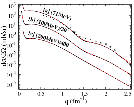
Figure 3: (Color online) The angular distribution of the differential cross section, $\frac{d\sigma}{d\Omega}$, for elastic scattering of ⁶He at projectile energies [a] 71 MeV/nucleon, [b] 100 MeV/nucleon/40, and [c] 200 MeV/nucleon/400 as function of the momentum transfer. The calculations are performed with an optical potential based on the CD-Bonn potential. The solid line represents the full calculations, while the dash-dotted line represents the calculating omitting open-shell effects. The data are taken from Refs. Uesaka et al. (2010); Korsheninnikov et al. (1997)

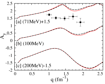
Figure 4: (Color online) The angular distribution of the analyzing power ($A_{y}$) for elastic scattering of ⁶He at projectile energies [a] 71 MeV/nucleon, [b] 100 MeV/nucleon, and [c] 200 MeV/nucleon as function of the momentum transfer. The values for [a] and [c] are shifted as indicated in the figure. The meaning of the lines is the same as in Fig. 3. The data are taken from Ref. Uesaka et al. (2010); Sakaguchi et al. (2011).

In order to study the effect of those two additional term we first calculate the differential cross section, $d\sigma/d\Omega$, and the analyzing power, $A_{y}$, for scattering of ⁶He from a polarized proton target using a a folding optical potential based only on the traditionally used central and spin-orbit terms corresponding to the Wolfenstein amplitudes $A$ and $C$. Those calculations are shown by the dashed lines in Fig. 3 for the differential cross section and Fig. 4 for the analyzing power. Our calculations are carried out for 71, 100 and 200 MeV per nucleon, and use the CD-Bonn potential Machleidt (2001) as NN interaction. Then we add the two additional contributions from the valence neutrons to the optical potential and show those calculations as solid lines in Figs. 3 and 4. First we notice, that the differential cross section is completely insensitive the additional terms. This might be expected since the expectation value ${\tilde{\rho}}$ is an order of magnitude smaller than the single-particle density matrix. However, the effect of additional contribution to the spin-orbit potential through the Wolfenstein amplitude $M$ is also very small. We note, that there is also a small effect on $A_{y}$ through the change in the central potential. However, both effects are so small, that they do not warrant to be shown separately.

In closing this section, we want to comment on final state interactions resulting from the breakup of the ⁶He on the scattering process. The effect of final state interactions in a proton-nucleus optical potential was studied in Ref. Elster and Weppner (1998) for closed shell nuclei, with ¹⁶O being the lightest nucleus, for projectile energies between 65 and 200 MeV. This study concluded that for projectile energies of 100 MeV and above there was no effect, and at 65 MeV it was very small. We expect that this conclusion will also hold in the case of ⁶He scattering off a proton target, since in this case the breakup of ⁶He would lead to a $np$ final state interaction, which is strongest when the $np$ system is in an s-wave and the relative energy of the $np$-pair is less than 10 MeV. Even the lowest energy we consider, namely 71 MeV, is sufficiently high, that we are quite certain that $np$ final state interactions are too small to affect the results of our calculations.

III Sensitivity of the ⁶He Scattering Observables to the Functional Form of the Wave Function for large Radii

In the previous section we calculated additional contributions to the optical potential for ⁶He due to the two valence neutrons occupying the p_3/2 ground state, and find that their effect on the observables for elastic scattering is very small. We use a very simple ansatz for the single-particle density matrix, namely only two harmonic oscillator functions, which may lead to this very small contribution. A further point of concern is the asymptotic behavior of the harmonic oscillator wave functions, which do not correctly capture the halo character of the ⁶He nucleus. Therefore, we need to investigate, if the behavior of the wave functions for large values of $r$, i.e. the tail of the coordinate space wave function, can be seen in the scattering observables at the energies we consider. For the calculation of S-factors, i.e. at very low energies, it is well known that the asymptotic form of the nuclear wave functions is very important Navratil et al. (2006). We need to carry out a similar investigation for our calculations.

Considerations about the asymptotic behavior of the single-particle wave functions are most naturally carried out in coordinate space, though we will have to define some ‘equivalent’ in momentum space. Following a similar line of thought as Ref. Navratil et al. (2006) we define the radial part of the p-shell wave function as

$$\Phi^{radial}_{p}(r)=\left(2\sqrt{\frac{1}{6}}\;\frac{r\;\nu_{p}^{5/4}}{\pi^{1/4}}\;e^{\left(-\frac{r^{2}\;\nu_{p}}{2}\right)}\bigg{|}_{r\leq R_{m}}+B\;e^{-\mu\;r}\bigg{|}_{r>R_{m}}\right)$$ (65)

Here $R_{m}$ is the matching radius, at which we match the harmonic oscillator p-wave and its derivative with an exponential tail. The parameter $\mu$ should in principle be close to the two-nucleon separation energy of the valence neutrons. The oscillator parameters are $\nu_{s}=0.392$ fm^-1 and $\nu_{p}=0.289$ fm^-1.

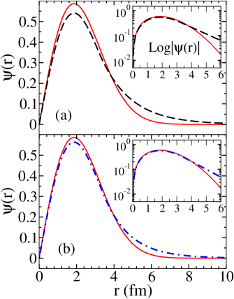
Figure 5: (Color online) The coordinate space p-shell wave function of ⁶He. The solid (red) line represents a harmonic oscillator wave functions. For the dashed (black) line in panel (a) an exponential functions was matched at $R_{m}$ = 3.2 fm, while for the dash-dotted (blue) line in panel (b) an exponential function was matched at $R_{m}$ = 3.5 fm.

For determining reasonable values for $R_{m}$ we want to assume, that the alpha-core of ⁶He shall not be significantly affected by changing the behavior of the p-wave. Thus we ensure that for fixed $R_{m}$ the integral over the s-wave harmonic oscillator function contains most of the mass of the alpha core. The s-shell probability is given in Table 2 as function of $R_{m}$. The values for the s-shell probability show, that for $R_{m}\geq 3.2$ fm more than 95% of the alpha core are being described by the s-wave oscillator function, and thus the core is minimally affected by the matching procedure. For $R_{m}=3.2$ fm about 69% of the probability for the valence neutrons is described by the p-shell oscillator wave function, the remaining by the exponential tail. Normalizing this hybrid p-wave leads to a norm of 2.35, and we have to renormalize the p-wave to two, the number of neutrons in the p-shell. Choosing $R_{m}=3.5$ fm leaves almost the entire alpha-core unmodified, describes about 79% of the valence neutrons by the harmonic oscillator p-wave, and gives a norm of 2.17. Table 2 shows in addition those values for $R_{m}=2.8$ fm and $R_{m}=3.8$ fm. The small value of $R_{m}$ gives a p-shell norm of three, which means that there would be three valence neutrons. For this reason we consider $R_{m}=2.8$ fm as too small a matching radius. The highest value in Table 2 is $R_{m}=3.8$ fm, which we consider a bit large for studying effects of a change in the p-wave tail. We included the values in the table, to support our arguments for choosing $R_{m}=3.2$ fm and $R_{m}=3.5$ fm for our study of the sensitivity to an exponential tail of the p-wave on the scattering observables. The coordinate space p-shell wave functions for those two cases are shown in Fig. 5 in comparison with the original harmonic oscillator p-wave. For completeness Table 2 also contains the matter radii $r_{mat}$ calculated with the modified p-waves. Once the parameters $\mu$ and $B$ for the exponential tail are determined through matching the logarithmic derivative at $R_{m}$ and renormalizing the p-wave probability to two neutrons, the matter radius is a predictive quantity.

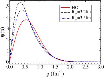
Figure 6: (Color online) The momentum space p-shell wave function of ⁶He. The solid (red) line represents a harmonic oscillator wave function, while for the dashed (black) line an exponential function was matched at $R_{m}$ = 3.2 fm, and for the dash-dotted (blue) line an exponential function was matched at $R_{m}$ = 3.5 fm.

For the momentum space calculations we need to Fourier transform the wave functions and renormalize them to the number of nucleons in ⁶He. The resulting momentum space p-waves are shown in Fig. 6 together with the original harmonic oscillator p-wave. This figure also indicates, that an exponential tail in coordinate space leads to a modification of the momentum space wave function for small momenta. From these wave functions we construct the single-particle density matrix and calculate the microscopic folding optical potential.

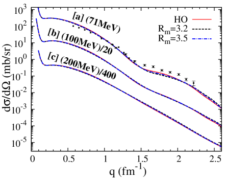
Figure 7: (Color online) The angular distribution of the differential cross section, $\frac{d\sigma}{d\Omega}$, for elastic scattering of ⁶He at projectile energies [a] 71 MeV/nucleon, [b] 100 MeV/nucleon/40, and [c] 200 MeV/nucleon/400 as function of the momentum transfer. The calculations are performed with an optical potential based on the CD-Bonn potential. The solid (red) line represents the full calculations based on Harmonic Oscillator densities, while the dashed (black) line represents a calculation in which the p-shell neutron wave functions have been matched at $R_{m}$ = 3.2 fm with an exponential wave function. For the dash-dotted (blue) line this matching radius is $R_{m}$ = 3.m fm. The data are taken from Refs. Uesaka et al. (2010); Korsheninnikov et al. (1997)

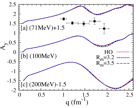
Figure 8: (Color online) The angular distribution of the analyzing power ($A_{y}$) for elastic scattering of ⁶He at projectile energies [a] 71 MeV/nucleon, [b] 100 MeV/nucleon, and [c] 200 MeV/nucleon as function of the momentum transfer. The values for [a] and [c] are shifted as indicated in the figure. The meaning of the lines is the same as in Fig. 7. The data are taken from Ref. Uesaka et al. (2010); Sakaguchi et al. (2011).

The calculations of the differential cross section for 71, 100, and 200 MeV per nucleon are shown in Fig. 7. The figure shows that the different exponential tails of the p-wave have no effect on this observable. In Fig. 8 we show the corresponding calculations of the angular distribution of the analyzing power. Again, the exponential form of the p-wave tail has no effect on this observable.

The different functional of the tail of the coordinate space p-wave translates into differences in the p-wave for small momentum p for the momentum space p-wave. Our calculations of the scattering observables for projectile energies from 71 to 200 MeV per nucleon show, that for these energies the affected small momenta of the single-particle density have no effect on the observables. This conclusion is quite different from the one in Ref.Navratil et al. (2006) in which the extraction of S-factors from reactions below 1 MeV was investigated. These two finding are not in contradiction, since at very low energies, reactions are expected to be mostly sensitive to the long range part of wave functions, whereas for the higher energy regime considered in this work, the asymptotic part of the wave functions, and thus single particle density matrices should play a lesser role.

IV Sensitivity of the Scattering Observables to the Charge and Matter Radii of ⁶He

After establishing that at the scattering energies under consideration the fall-off behavior of the wave functions in coordinate space has no significant effect on the scattering observables, we should study if other input parameters into our model lead to discernible effects. In Section II.3 we presented calculations for the differential cross section and the analyzing power using oscillator parameters from Table 1. Over the last years there have been several measurements of the charge radius of ⁶He. Our model density uses the charge radius to determine the oscillator parameter $\nu_{s}$ for the s-shell single particle density according to Eq. (43). The s-shell single particle density determines the size of the alpha-core in our model, and therefore we want to test, how sensitive the elastic scattering observables are to changes in $\langle r^{2}_{ch}\rangle$. As limits for this check we use the measurement of Ref. Wang et al. (2004), which obtained a charge radius of 1.894 fm as lower limit and the value of 1.996 fm Mueller et al. (2007) as upper limit.

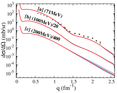
Figure 9: (Color online) The angular distribution of the differential cross section, $\frac{d\sigma}{d\Omega}$, for elastic scattering of ⁶He at projectile energies [a] 71 MeV/nucleon, [b] 100 MeV/nucleon/40, and [c] 200 MeV/nucleon/400 as function of the momentum transfer. The solid (red) line corresponds to the same calculation as the solid line in Fig. 3, which which gives a charge radius $r_{ch}$ = 1.955 fm and a matter radius $r_{mat}$ = 2.33 fm. The shaded region shows the variation of the charge radius from 1.89 fm to 1.99 fm. The data are taken from Refs. Uesaka et al. (2010); Korsheninnikov et al. (1997)

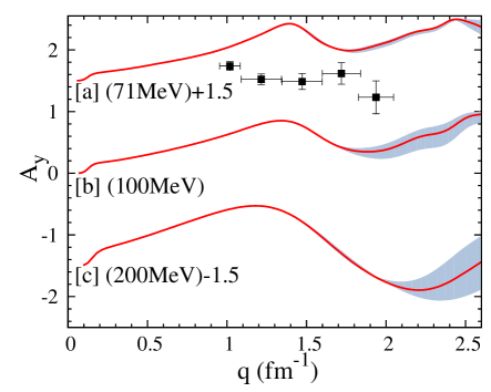
Figure 10: (Color online) The angular distribution of the analyzing power ($A_{y}$) for elastic scattering of ⁶He at projectile energies [a] 71 MeV/nucleon, [b] 100 MeV/nucleon, and [c] 200 MeV/nucleon as function of the momentum transfer. The values for [a] and [c] are shifted as indicated in the figure. The meaning of the lines is the same as in Fig. 9. The data are taken from Ref. Uesaka et al. (2010); Sakaguchi et al. (2011).

The sensitivity to the variation in $\langle r^{2}_{ch}\rangle$, which translates to a variation of $\nu_{s}$ is shown in Fig. 9 for the differential cross section as function of momentum transfer for the different scattering energies. Since the difference between the measured values of the charge radius is quite small, the variations in the differential cross section are also quite small. Since the charge radius also enters the relation of the parameters $\nu_{s}$ and $\nu_{p}$ and the matter radius $\langle r^{2}_{mat}\rangle$, Eq. (44), we keep the matter radius constant at 2.33 fm. The angular distribution of the analyzing power is shown in Fig. 10 as function of the momentum transfer for the same three scattering energies. Here a larger sensitivity to the size of the charge radius is visibly for momentum transfers $q\geq 2\rm{fm}^{-1}$ as indicated by the shaded region. The sensitivity is larger for the higher scattering energies, indication that at those energies more of the interior, i.e. the alpha-core, of ⁶He is probed. Nevertheless, the variations are relatively small even at 200 MeV/nucleon, and probably not experimentally accessible.

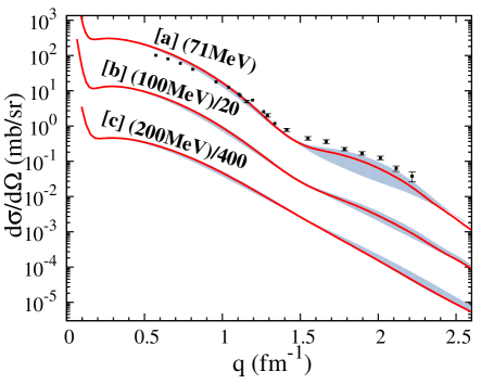
Figure 11: (Color online) The angular distribution of the differential cross section, $\frac{d\sigma}{d\Omega}$, for elastic scattering of ⁶He at projectile energies [a] 71 MeV/nucleon, [b] 100 MeV/nucleon/40, and [c] 200 MeV/nucleon/400 as function of the momentum transfer. The solid (red) line corresponds to the same calculation as the solid line in Fig. 3, which which gives a charge radius $r_{ch}$ = 1.955 fm and a matter radius $r_{mat}$ = 2.33 fm. The shaded region shows the variation of the matter radius from 2.24 fm to 2.60 fm. The data are taken from Refs. Uesaka et al. (2010); Korsheninnikov et al. (1997)

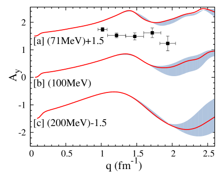
Figure 12: (Color online) The angular distribution of the analyzing power ($A_{y}$) for elastic scattering of ⁶He at projectile energies [a] 71 MeV/nucleon, [b] 100 MeV/nucleon, and [c] 200 MeV/nucleon as function of the momentum transfer. The values for [a] and [c] are shifted as indicated in the figure. The meaning of the lines is the same as in Fig. 11. The data are taken from Ref. Uesaka et al. (2010); Sakaguchi et al. (2011).

The matter radius is an extracted quantity and less well known than the charge radius. For testing the sensitivity of the scattering observables to the matter radius we keep the charge radius fixed at 1.995 fm. As lower limit for the matter radius we choose the value of 2.24 fm extracted in Ref. Bacca et al. (2012) and as upper limit the value of 2.6 fm used in Ref. Kaki et al. (2012). The sensitivity of the differential cross section to the variation of the matter radius in these limits is shown in Fig. 11 for three different scattering energies. Here it is interesting to note that the lowest scattering energy, 71 MeV / nucleon, shows the strongest sensitivity in the region between 1.5 and 2 fm^-1, indicated by the shaded region. This most likely results from the fact that the matter radius is dominated by the two outer valence neutrons. The figure further indicates as far as our model is concerned, the data favor the smaller values of the matter radius. In Fig. 12 we show the sensitivity of the analyzing power to the same variation of the matter radius. It is interesting to observe, that the analyzing power is less sensitive to the variation of the matter radius than the differential cross section. However, this may be an artefact of our model, which puts the to valence neutrons into the p_3/2-shell. Again the two higher energies show considerably more sensitivity to variations in the matter radius for momentum transfers $q\geq 2\rm{fm}^{-1}$ as indicated by the shaded region in Fig. 11.

V Open Shell Effects in the Optical Potential in ⁸He

The single particle density of ⁶He introduced in Section II.1 can be readily extended to the single particle density of ⁸He. The p_3/2 shell can be occupied by four valence neutrons coupled to total spin zero. Both helium isotopes have an alpha core, thus the relation between the s-shell oscillator parameter $\nu_{s}$ and the charge radius of Eq. (43) is the same. The parameter $\nu_{s}$ determined from the measured charge radius Brodeur et al. (2012) for ⁸He is given in Table 1. The relation between the matter radius and the parameters $\nu_{s}$ and $\nu_{p}$ is modified for ⁸He to

$$\langle r^{2}_{mat}\rangle=\frac{1}{8}\left(\frac{10}{\nu_{p}}+\frac{6}{\nu_{s}}\right).$$ (66)

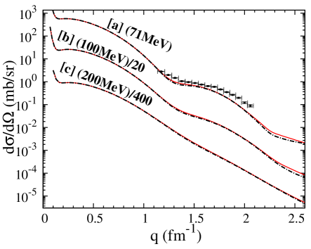
Figure 13: (Color online) The angular distribution of the differential cross section, $\frac{d\sigma}{d\Omega}$, for elastic scattering of ⁸He at projectile energies [a] 71 MeV/nucleon, [b] 100 MeV/nucleon/40, and [c] 200 MeV/nucleon/400 as function of the momentum transfer. The calculations are performed with an optical potential based on the CD-Bonn potential. The solid line represents the full calculations, while the dash-dotted line represents the calculating omitting open-shell effects.

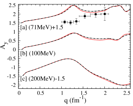
Figure 14: (Color online) The angular distribution of the analyzing power ($A_{y}$) for elastic scattering of of ⁸He at projectile energies [a] 71 MeV/nucleon, [b] 100 MeV/nucleon, and [c] 200 MeV/nucleon as function of the momentum transfer. The values for [a] and [c] are shifted as indicated in the figure. The meaning of the lines is the same as in Fig. 13.

Our calculations use the value of 2.53 fm from Ref. Tanihata et al. (1992) as matter radius. Since in ⁸He the p_3/2-shell is occupied by double the amount of neutrons as the one in ⁶He, one may speculate that the effect of the extra terms in the microscopic optical potential resulting from these neutrons is larger compared to ⁶He. To investigate this we first calculate the microscopic optical potential using only the terms generated by the Wolfenstein amplitudes $A$ and $C$, and then compare to the corresponding calculations based on the the expression of Eq. (64). In Fig. 13 this comparison is shown for the differential cross section for scattering of ⁸He off a proton target as function of the momentum transfer for three selected energies. The effect of the additional terms in Eq. (64) are here vanishingly small. The corresponding comparison for the analyzing power as function of the momentum transfer is depicted in Fig. 14. The figure shows that the additional terms in the optical potential due the four valence neutrons of ⁸He are in the same order of magnitude as shown in Fig. 4 for the analyzing power of ⁶He. The reason may here be also that our model for the single-particle density with only two oscillator wave functions is too simple.

VI Summary and Conclusions

In this work we extended the traditionally employed formulation of the first-order microscopic optical potential for elastic scattering from closed shell nuclei to nuclei with partially filled shells. The complete full-folding integral for this first-order optical potential has been carried out with the simplifying assumption that the single-particle density matrix for ⁶He and ⁸He is given by a simple harmonic oscillator model. The alpha-core is described by a single particle density matrix derived from one s-shell harmonic oscillator function, while the two valence neutrons occupy the p_3/2-shell and are in the ground state coupled to spin zero. The corresponding single particle density matrix is also derived from a single p-shell harmonic oscillator function.

With these assumptions all terms of the optical potential that arise when integrating the six fully-off-shell Wolfenstein amplitudes of the NN scattering amplitude with the single particle density matrix are derived and calculated. It turns out, that those Wolfenstein amplitudes that are related to the NN tensor force, namely $G$, $H$, and $D$ do not contribute to optical potential when employing our model ansatz for the single particle density matrix, in which the ground state consists of the two valence neutrons occupying the p_3/2-shell. With our model single particle density the ‘traditional’ first-order microscopic folding optical potential, which consists of a central term related to the Wolfenstein amplitude $A$ and a spin-orbit term related to the Wolfenstein amplitude $C$, acquires two new additional terms. One of those terms is related to the Wolfenstein amplitude $C$, but since it does not contain any spin-dependence, it adds to the central part of the optical potential. The other term, which is related to the Wolfenstein amplitude $M$ adds to the spin-orbit part of the optical potential.

With these first-order folding optical potentials for ⁶He and ⁸He we calculated the observables for elastic scattering, i.e. the differential cross section and the analyzing power, at 71, 100, and 200 MeV per nucleon. We find that in all cases the additional terms have a very small effect on the observables. This is most likely result from the simplicity of our model ansatz for the ground states of the two helium isotopes. Thus, we do not think it appropriate to make a general conclusion about the importance of explicitly treating open shell structure in a microscopic optical potential. However, we would like to point out, that our derivations open the path for employing sophisticated ground state wave functions into a microscopic folding optical potential, as the ones provided by the no-core shell-model Navratil et al. (2009); Cockrell et al. (2012) (NSCM). In the NSCM the ground state of light nuclei is calculated in a large $\hbar\Omega$ space. This leads to additional contributions for each angular momentum state included in the NSCM. In addition, in a large $\hbar\Omega$ space transitions between different $l$ states will be allowed. Terms containing the Wolfenstein amplitudes $G+H$ and $D$, which do not contribute in the simple $s$- and $p_{3/2}$-shell model employed in this work, will contribute whenever $l\neq l^{\prime}$ transitions are included. In this case all Wolfenstein amplitudes will contribute. As further remark, a NSCM single particle density matrix can be most naturally included in this formulation of the first-order microscopic folding optical potential, since it is quite straightforward to derive a translationally invariant single particle density using the NSCM Navratil (2004).

We also want to point out that the formulation of a general spin-dependent single particle density matrix of Section II.1 allows to consider not only optical potential for the helium-isotopes as done in this work. The formulation is written down for nuclear single particle densities with arbitrary spin.

Since ⁶He and ⁸He are both halo nuclei, with a small separation energy of the two valence neutron, and thus a large spatial extension, we needed to investigate if our model ansatz based on harmonic oscillator wave functions is inappropriate as input for the optical potential. More specifically, we needed to investigate if an exponentially decreasing spatial density, which is characteristic for halo nuclei, would yield significantly different results for the scattering observables. We carried out this investigation by matching an exponential tail at radii of about 3 fm to the oscillator waver functions. The Fourier transform of these hybrid wave functions, after renormalization to the particle number, was used to derive single particle densities. We find, that at the scattering energies under consideration, the observables are not sensitive to the long-range tail of the wave functions of the valence neutrons. This is a very encouraging result for plans to use no-core shell-model single particle densities in calculating first-order optical potentials.

Last, we performed a sensitivity study of the scattering observables to the charge and matter radii of ⁶He. The charge radius of ⁶He is experimentally quite well known, and thus when varying the s-wave oscillator parameter within the boundaries dictated by experiment, we did not find a large variation in the observables. The situation is slightly different for the matter radius, since this is often an extracted quantity, and we had a larger range of variation. We found that the differential cross section at 71 MeV per nucleon preferred a matter radius towards the smaller side of the values we considered. The analyzing power at 100 and 200 MeV per nucleon shows sensitivity with respect to the matter radius for momentum transfers $q\geq 2~{}{\rm fm}^{-1}$. The planned experiment at RIKEN at this energy may be able to reach a momentum transfer of that size.

Appendix A Calculation of the Expectation Values

In this appendix we give some details of the evaluation of the spin-momentum operator of the scattering amplitude ${\overline{M}}$ of Eq. 7 in the target intrinsic frame. For the evaluation we define the spin operator as

$$\mbox{\boldmath$\sigma$}\equiv(\sigma_{1},\sigma_{2},\sigma_{3})\equiv(\frac{\sigma_{+}-\sigma_{-}}{2i},\sigma_{3},\frac{\sigma_{+}+\sigma_{-}}{2}),$$ (67)

where the superscript $i$ is omitted since only the struck target nucleon is considered, and $\sigma_{\pm}=\sigma_{1}\pm i\sigma_{2}$. As indicated in Ref. Elster et al. (1990), in case of closed shell nuclei, the sum over all states leads to a zero contribution of the spin-momentum operators. Considering the explicit expression of Eq. (34) for the p_3/2 wave function of the two valence neutrons coupled to total spin zero, we obtain when only considering the angular momentum parts

$$\Phi_{p}({\hat{{\bf{p}}}}^{\prime})\;\mbox{\boldmath$\sigma$}^{(i)}\cdot{\hat{{\bf{n}}}}_{TI}\;\Phi_{p}({\hat{{\bf{p}}}})$$ (68)

$$= \frac{1}{12}\Big{(}\frac{\hat{n}_{3}}{\sqrt{2}}\left(Y_{1}^{0}({\hat{{\bf{p}}}}^{\prime})\left\{Y_{1}^{1}({\hat{{\bf{p}}}})+Y_{1}^{-1}({\hat{{\bf{p}}}})\right\}-\left\{Y_{1}^{1}({\hat{{\bf{p}}}}^{\prime})+Y_{1}^{-1}({\hat{{\bf{p}}}}^{\prime})\right\}Y_{1}^{0}({\hat{{\bf{p}}}})\right)$$ (69)

$$+ 2\hat{n}_{2}\left(Y_{1}^{1}({\hat{{\bf{p}}}}^{\prime})Y^{-1}_{1}({\hat{{\bf{p}}}})-Y^{-1}_{1}({\hat{{\bf{p}}}}^{\prime})Y_{1}^{1}({\hat{{\bf{p}}}})\right)$$ (70)

$$+ \frac{i\hat{n}_{1}}{\sqrt{2}}\left(Y_{1}^{0}({\hat{{\bf{p}}}}^{\prime})\left\{Y_{1}^{-1}({\hat{{\bf{p}}}})-Y_{1}^{1}({\hat{{\bf{p}}}}\right\}+\left\{Y_{1}^{1}({\hat{{\bf{p}}}}^{\prime})-Y_{1}^{-1}({\hat{{\bf{p}}}}^{\prime})\right\}Y_{1}^{0}({\hat{{\bf{p}}}})\right)\Big{)}$$ (71)

The same form of expression is obtained when replacing ${\hat{{\bf{n}}}}_{TI}$ with ${\hat{{\bf{q}}}}_{TI}$ and ${\hat{{\bf{P}}}}_{TI}$. Eq. (71) is obtained in the target intrinsic frame, which can be oriented arbitrarily with respect to other frames. Therefore it is necessary to integrate over all possible orientations of the target frame relative to the nucleon-nucleus frame, i.e. evaluate

$$I=\frac{1}{8\pi^{2}}\int d{\hat{{\bf{p}}}}{\hat{{\bf{p}}}}^{\prime}\Phi_{p}({\hat{{\bf{p}}}}^{\prime})\;\mbox{\boldmath$\sigma$}^{(i)}\cdot{\hat{{\bf{n}}}}_{TI}\;\Phi_{p}({\hat{{\bf{p}}}})\;\delta({\hat{{\bf{p}}}}\cdot{\hat{{\bf{p}}}}^{\prime}-\cos\alpha_{pp^{\prime}}),$$ (72)

where the factor $8\pi^{2}$ is the norm of the integral with respect to a fixed angle between the vectors ${\hat{{\bf{p}}}}$ and ${\hat{{\bf{p}}}}^{\prime}$. The delta function keeps the angle between ${\hat{{\bf{p}}}}$ and ${\hat{{\bf{p}}}}^{\prime}$ fixed and can be expressed as

$$\cos\alpha_{pp^{\prime}}=\cos\theta^{\prime}\cos\theta+\sin\theta^{\prime}\sin\theta\;\cos(\phi-\phi^{\prime})$$ (73)

When the angle is fixed for a given ${\hat{\bf p}}^{\prime}$, allowed orientations of the unit vector ${\hat{{\bf{p}}}}$ form a cone. The projection of the cone’s base onto the $xy$ plane is an ellipse centered at

$$X_{c} = \sin\theta^{\prime}\cos\phi^{\prime}\cos\alpha_{pp^{\prime}}$$ (74)

$$Y_{c} = \sin\theta^{\prime}\sin\phi^{\prime}\cos\alpha_{pp^{\prime}}.$$ (75)

With the major and minor axes given as $a=\sin\alpha_{pp^{\prime}}$ and $b=\cos\theta^{\prime}\sin\alpha_{pp^{\prime}}$ the parametric equation of the ellipse is determined as

$$x = X_{c}+a\;\cos t\cos(\pi/2+\phi^{\prime})-b\;\sin t\sin(\pi/2+\phi^{\prime})$$ (76)

$$y = Y_{c}+a\;\cos t\sin(\pi/2+\phi^{\prime})+b\;\sin t\cos(\pi/2+\phi^{\prime}).$$ (77)

The spherical harmonics depend on the angles $\theta$ and $\phi$, thus the integration over the solid angle $\Omega$ can be replaced by the integration over the parameter $t$,

$$\int d\Omega\;\int d\Omega^{\prime}\;Y^{m_{1}}_{m_{1}}({\hat{{\bf{p}}}}^{\prime})Y{m_{2}}_{m_{1}}({\hat{{\bf{p}}}})\;\delta({\hat{p}}\cdot{\hat{p}}^{\prime}-\cos\alpha_{pp^{\prime}})=\int d\Omega^{\prime}\int\limits_{0}^{2\pi}dtY^{m_{1}}_{m_{1}}({\hat{{\bf{p}}}}^{\prime})Y{m_{2}}_{m_{1}}({\hat{{\bf{p}}}}).Y_{1}^{m2}({\hat{{\bf{p}}}})$$ (78)

Substituting Eqs. (71) and (72) and integrating leads to

$${\tilde{\rho}}_{p}({\bf{p}},{\bf{p}}^{\prime})=-i\>\frac{2}{9}\frac{1}{\sqrt{\pi^{3}\nu_{p}^{5}}}\;|{\bf{p}}\times{\bf{p}}^{\prime}|\;e^{-\frac{p^{2}+p^{\prime 2}}{2\nu_{p}}},$$ (79)

which leads to Eq. (56) after transforming to the variable ${\bf q}$ and P.

For calculating the expectation value of $\mbox{\boldmath$\sigma$}^{(i)}\cdot{\hat{{\bf{q}}}}$ the same procedure is applied. Here we only have to consider that

$$|q|=\sqrt{p^{2}+p^{\prime 2}-2|p||p^{\prime}|\cos\alpha_{pp^{\prime}}}$$ (80)

and the unit vector ${\hat{\bf q}}$ as function of the angles $(\theta,\phi)$ and $(\theta^{\prime},\phi^{\prime})$ is given as

$${\hat{{\bf{q}}}}=\frac{1}{|q|}\left(\begin{array}[]{cc}|p|\sin\theta\cos\phi-|p^{\prime}|\sin\theta^{\prime}\cos\phi^{\prime}\\ |p|\sin\theta\sin\phi-|p^{\prime}|\sin\theta^{\prime}\sin\phi\\ |p|\cos\theta-|p^{\prime}|\cos\theta^{\prime}\end{array}\right).$$ (81)

Inserting this into the corresponding integral, Eq. (72) leads to

$$\frac{1}{8\pi^{2}}\int d{\hat{{\bf{p}}}}d{\hat{{\bf{p}}}}^{\prime}\Phi_{p}({\hat{{\bf{p}}}}^{\prime})\;\mbox{\boldmath$\sigma$}^{(i)}\cdot{\hat{{\bf{q}}}}\;\Phi_{p}({\hat{{\bf{p}}}})\;\delta({\hat{{\bf{p}}}}\cdot{\hat{{\bf{p}}}}^{\prime}-\cos\alpha_{pp^{\prime}})=0$$ (82)

The same integral for ${\bf P}$ also gives a zero contribution.

Appendix B Explicit Calculation of Contribution from the Wolfenstein amplitudes G+H, and D

As indicated in Eqs. (61) and (63), the contributions of the Wolfenstein amplitudes $G+H$ and $D$ vanish. In this appendix the explicit calculation is given. The structure of the different terms in Eq. (61) can be summarized as

$$U_{1} = \int d^{3}P\;(G+H)\;\frac{1}{|K_{NN}|}\;|k_{NN}|\;\cos\alpha\;\tilde{\rho}({\bf{q}},{\bf{P}})$$ (83)

$$U_{2} = \int d^{3}P\;(G+H)\;\frac{1}{|K_{NN}|}\;|k_{NN}^{\prime}|\cos\gamma_{NN}\;\cos\alpha\;\tilde{\rho}({\bf{q}},{\bf{P}})$$ (84)

$$U_{3} = \int d^{3}P\;(G+H)\;\frac{1}{|K_{NN}|}\;|k_{NN}^{\prime}|\sin\gamma_{NN}\;\cos\alpha\;\tilde{\rho}({\bf{q}},{\bf{P}})$$ (85)

and for Eq. (63) as

$$U_{4} = \int d^{3}P\;D\;\frac{1}{|q|}\;|k_{NN}|\;\cos\alpha\;\tilde{\rho}({\bf{q}},{\bf{P}})$$ (86)

$$U_{5} = \int d^{3}P\;D\;\frac{1}{|q|}\;|k_{NN}^{\prime}|\cos\gamma_{NN}\;\cos\alpha\;\tilde{\rho}({\bf{q}},{\bf{P}})$$ (87)

$$U_{6} = \int d^{3}P\;D\;\frac{1}{|q|}\;|k_{NN}^{\prime}|\sin\gamma_{NN}\;\cos\alpha\;\tilde{\rho}({\bf{q}},{\bf{P}}),$$ (88)

where the integration explicity reads $\int d^{3}P=\int_{0}^{\infty}P^{2}dP\int_{-1}^{1}d\cos\theta_{P}\int_{0}^{2\pi}d\phi_{P}$. We can show that the integrands are odd functions of the azimuthal angle $\phi_{P}$, and thus the integrals in Eq. (85) and (88) vanish. In order to show this, we first note that $\tilde{\rho}({\bf{q}},{\bf{P}})$ from Eq. (56) contains the cross product $|{\bf q}\times{\bf P}|$ and thus depends on $\sin\theta_{P}$. Next we need to explicitly consider the term in Eq. (85), The magnitude of the vector ${\bf{K}}_{NN}$ is given by

$$|K_{NN}|=\frac{1}{2}\sqrt{P^{2}+\left(\frac{A+1}{A}\right)^{2}K^{2}-2\frac{A+1}{A}|P||K|\cos\gamma_{PK}}.$$ (89)

Applying the addition theorem of spherical harmonics for $l=1$, $\cos\gamma_{PK}$ can be expressed as

$$\cos\gamma_{PK}=\cos\theta_{P}\cos\theta_{K}+\sin\theta_{P}\sin\theta_{K}\cos\phi_{P}.$$ (90)

Thus, Eq. (89) can be re-expressed as

$$|K_{NN}|=\sqrt{a-b\cos\phi_{P}},$$ (91)

with

$$a = \frac{1}{4}\left(P^{2}+\left(\frac{A+1}{A}\right)^{2}K^{2}-2\frac{A+1}{A}|P||K|\cos\theta_{P}\cos\theta_{K}\right)$$ (92)

$$b = \frac{1}{2}\frac{A+1}{A}|P||K|\sin\theta_{P}\sin\theta_{K}.$$ (93)

The angle $\cos\alpha$ which occurs in transformation between the NN and the target intrinsic frame is defined as

$$\cos\alpha\equiv\widehat{{\bf{q}}\times{\bf{P}}}\cdot\hat{\mathbf{K}}_{NN}=\frac{1}{2\sin\theta_{P}}\frac{A+1}{A}\frac{1}{|q||P||K_{NN}|}\sum_{i=1}^{3}\sum_{j=1}^{3}\sum_{k=1}^{3}\;\epsilon_{ijk}\;K_{i}\;q_{j}\;P_{k}.$$ (94)

Choosing the reference frame such that ${\bf q}$ points along the z-axis,

$${\bf{q}}=(0,\;0,\;|q|);\;\;\;{\bf{K}}=(K_{x},\;0,\;K_{z});\;\;\;{\bf{P}}=(P_{x},\;P_{y},\;P_{z}),$$ (95)

one obtains for Eq. (94)

$$\cos\alpha=-\frac{|K|\sin\theta_{K}}{2}\frac{A+1}{A}\frac{\sin\phi_{P}}{\sqrt{a-b\cos\phi_{P}}},$$ (96)

The magnitudes of the vectors ${\bf{k}}_{NN}$ and ${\bf{k}}_{NN}^{\prime}$ are given as

$$|k_{NN}^{\prime}| = \sqrt{K_{NN}^{2}+\frac{q^{2}}{4}+|K_{NN}||q|\cos\theta_{K_{NN}}}$$ (97)

$$|k_{NN}| = \sqrt{K_{NN}^{2}+\frac{q^{2}}{4}-|K_{NN}||q|\cos\theta_{K_{NN}}},$$ (98)

with

$$\cos\theta_{K_{NN}}=\frac{{\bf{q}}\cdot{\bf{K}}_{NN}}{|q||K_{NN}|}=\frac{1}{2|K_{NN}||q|}\>{\bf{q}}\cdot\left(\frac{A+1}{A}{\bf{K}}-{\bf{P}}\right)\equiv\frac{c}{\sqrt{a-b\cos\phi_{P}}},$$ (99)

where

$$c=\frac{1}{2}\left(\frac{A+1}{A}|K|\cos\theta_{K}-|P|\cos\theta_{P}\right).$$ (100)

Introducing the abbreviations

$$a_{1}^{\prime} = a+\frac{q^{2}}{4}+\frac{|q|}{2}\left(\frac{A+1}{A}|K|\cos\theta_{K}-|P|\cos\theta_{P}\right)$$ (101)

$$a_{1} = a+\frac{q^{2}}{4}-\frac{|q|}{2}\left(\frac{A+1}{A}|K|\cos\theta_{K}-|P|\cos\theta_{P}\right),$$ (102)

Eq. (98) can be re-expressed as

$$|k_{NN}^{\prime}| = \sqrt{a_{1}^{\prime}-b\cos\phi_{P}}$$ (103)

$$|k_{NN}| = \sqrt{a_{1}-b\cos\phi_{P}}.$$ (104)

The angle $\cos\gamma_{NN}$ is given by

$$\cos\gamma_{NN} \equiv \frac{{\bf{k}}_{NN}\cdot{\bf{k}}_{NN}^{\prime}}{|k_{NN}||k_{NN}^{\prime}|}=\frac{a_{2}-b\cos\phi_{P}}{\sqrt{a_{1}^{\prime}-b\cos\phi_{P}}\;\sqrt{a_{1}-b\cos\phi_{P}}},$$ (105)

where $a_{2}=a-\frac{q^{2}}{4}$. Since $\sin\gamma_{NN}$ is obtained from $\cos\gamma_{NN}$, both functions depend on $\cos\phi_{P}$ and thus are even with respect to $\phi_{P}$.

The functional dependence of the Wolfenstein amplitudes $G$, $H$, and $D$ are explicitly given by e.g.

$$G({\bf{q}},{\bf{K}},\mathcal{E})\equiv G(|q|,|K_{NN}|,\;\cos\theta_{K_{NN}},\;\mathcal{E})=G(\left(|q|,\;\sqrt{a-b\cos\phi_{P}},\;\frac{c}{\sqrt{a-b\cos\phi_{P}}},\mathcal{E}\right)\equiv G(\phi_{P}).$$ (106)

Here we only give $G$. The functional dependence of $H$ and $D$ is exactly the same. Considering the symmetry properties of $G$, Eq. (106), we see that $G(\pi+\phi_{P})=G(\pi-\phi_{P})$. Thus when considering only the azimuthal part of the integration we obtain for $U_{1}$ of Eq. (85)

$$U_{1} = \int\limits_{0}^{2\pi}d\phi_{P}\;(G+H)\;\frac{\cos\alpha}{|K_{NN}|}\;|k_{NN}|$$ (107)

$$= \int\limits_{0}^{2\pi}d\phi_{P}\;(G+H)\left(|q|,\;\sqrt{a-b\cos\phi_{P}},\;\frac{c}{\sqrt{a-b\cos\phi_{P}}},\mathcal{E}\right)\;\frac{\sqrt{a_{1}-b\cos\phi_{P}}}{a-b\cos\phi_{P}}\sin\phi_{P}.$$ (108)

In this integration, for every point $\pi-\phi_{P}$ there is another point $\pi+\phi_{P},$ with the same value of $\cos\phi_{P}$. This means, the Wolfenstein amplitudes $G$, $H$, and $D$ have identical values at the points $\pi\pm\phi_{P}$. On the other hand, the $sine$ function is odd with respect to $\phi_{P}$. Therefore, the contribution of each point $\pi-\phi_{P}$ to the integral is canceled by the contribution of the point at $\pi+\phi_{P}$. Consequently, the overall integral is zero. The same argument applies to all other functions $U_{i}$ of Eqs. (85) and (88), which leads to the result that all integrals give zero, thus concluding our proof.

	$r_{ch}$ [fm]	$r_{mat}$ [fm]	$\nu_{s}$ [fm2]	$\nu_{p}$ [fm2]
6He	1.955 Mueller et al. (2007)	2.333 Wang (2004)	0.393	0.289
8He	1.885 Brodeur et al. (2012)	2.53 Tanihata et al. (1992)	0.422	0.270

Table 1: The charge and matter radii $r_{ch}$ and $r_{mat}$ used to determine the oscillator parameters for the density matrices of ⁶He and ⁸He.

$R_{m}$ [fm]	s-shell [%]	p-shell [%]	$\mu$ [fm-1]	B [fm-3]	norm (p-shell)	$r_{mat}$ [fm]
2.8	89.6	52.5	0.453	0.833	3.05	2.89
3.2	95.5	68.6	0.613	1.347	2.35	2.55
3.5	97.8	78.6	0.727	1.970	2.17	2.44
3.8	99.0	86.2	0.836	2.936	2.08	2.39

Table 2: Parameters for matching an exponential tail to the p-shell harmonic oscillator wave function. The detailed explanation of the parameters is given in Section III.