Model-free control

Abstract

“Model-free control” and the corresponding “intelligent” PID controllers (iPIDs), which already had many successful concrete applications, are presented here for the first time in an unified manner, where the new advances are taken into account. The basics of model-free control is now employing some old functional analysis and some elementary differential algebra. The estimation techniques become quite straightforward via a recent online parameter identification approach. The importance of iPIs and especially of iPs is deduced from the presence of friction. The strange industrial ubiquity of classic PID’s and the great difficulty for tuning them in complex situations is deduced, via an elementary sampling, from their connections with iPIDs. Several numerical simulations are presented which include some infinite-dimensional systems. They demonstrate not only the power of our intelligent controllers but also the great simplicity for tuning them.

Keywords:
Model-free control, PID controllers, intelligent PID controllers, intelligent PI controllers, intelligent P controllers, estimation, noise, flatness-based control, delay systems, non-minimum phase systems, fault accommodation, heat partial differential equations, operational calculus, functional analysis, differential algebra.

1 Introduction

Although model-free control was introduced only a few years ago (Fliess & Join (2008b, 2009); Fliess, Join & Riachy (2011b)), there is already a quite impressive list of successful concrete applications in most diverse fields, ranging from intelligent transportation systems to energy management (Abouaïssa, Fliess, Iordanova & Join (2012); Andary, Chemori, Benoit & Sallantin (2012); d’Andréa-Novel, Boussard, Fliess, el Hamzaoui, Mounier & Steux (2010); Choi, d’Andréa-Novel, Fliess, Mounier & Villagra (2009); De Miras, Riachy, Fliess, Join & Bonnet (2012); Formentin, de Filippi, Corno, Tanelli & Savaresi (2013); Formentin, de Filippi, Tanelli & Savaresi (2010); Gédouin, Delaleau, Bourgeot, Join, Arab-Chirani & Calloch (2011); Join, Masse & Fliess (2008); Join, Robert & Fliess (2010a, b); Lafont, Pessel, Balmat & Fliess (2013); Michel, Join, Fliess, Sicard & Chériti (2010); Milanes, Villagra, Perez & Gonzalez (2012); Sorcia-Vázquez, García-Beltrán, Reyes-Reyes & Rodríguez-Palacios (2010); Villagra, d’Andréa-Novel, Choi, Fliess, & Mounier (2009); Villagra & Balaguer (2011); Villagra & Herrero-Pérez (2012); Villagra, Milanés, Pérez & de Pedro (2010); Wang, Mounier, Cela & Niculescu (2011)). Most of those references lead to practical implementations. Some of them are related to patents.

Remark 1.1

The wording model-free control is of course not new in the literature, where it has already been employed by a number of authors. The corresponding literature is huge: see, e.g., Bilal Kadri (2009); Chang, Gao & Gu (2011); Hahn & Oldham (2012); Hong-wei, Rong-min & Hui-xing (2011); Keel & Bhattacharyya (2008); Killingsworth & Krstic (2006); Malis & Chaumette (2002); dos Santos Coelho, Wicthoff Pessôa, Rodrigues Sumar & Rodrigues Coelho (2010); Spall & Cristion (1998); Swevers, Lauwerys, Vandersmissen, Maes, Reybrouck & Sas (2007); Syafiie, Tadeo, Martinez & Alvarez (2011); Xu, Li & Wang (2012). The corresponding settings are quite varied. They range from “classic” PIDs to robust and adaptative control via techniques stemming from, e.g., neural nets, fuzzy systems, and soft computing. To the best of our understanding, those approaches are rather far from what we are developing here. Let us emphasize however Remark 1.5 for a comment on some works which are perhaps closer. See also Remark 1.3.

Let us now summarize some of the main theoretical ideas which are shaping our model-free control. We restrict ourselves for simplicity’s sake to systems with a single control variable $u$ and a single output variable $y$. The unknown “complex” mathematical model is replaced by an ultra-local model

$$\boxed{y^{(\nu)}=F+\alpha u}$$ (1)

1. $y^{(\nu)}$ is the derivative of order $\nu\geq 1$ of $y$. The integer $\nu$ is selected by the practitioner. The existing examples show that $\nu$ may always be chosen quite low, i.e., $1$, or, only seldom, $2$. See Section 4 for an explanation.

2. $\alpha\in\mathbb{R}$ is a non-physical constant parameter. It is chosen by the practitioner such that $\alpha u$ and $y^{(\nu)}$ are of the same magnitude. It should be therefore clear that its numerical value, which is obtained by trials and errors, is not a priori precisely defined. Let us stress moreover that controlling industrial plants has always been achieved by collaborating with engineers who know the system behaviour well.

3. $F$, which is continuously updated, subsumes the poorly known parts of the plant as well as of the various possible disturbances, without the need to make any distinction between them.

4. For its estimation, $F$ is approximated by a piecewise constant function. Then the algebraic identification techniques due to Fliess & Sira-Ramírez (2003, 2008) are applied to the equation

   $$y^{(\nu)}=\phi+\alpha u$$ (2)

   where $\phi$ is an unknown constant parameter. The estimation

   • necessitates only a quite short time lapse,

   • is expressed via algebraic formulae which contain low-pass filters like iterated time integrals,

   • is robust with respect to quite strong noise corruption, according to the new setting of noises via quick fluctuations (Fliess (2006)).

Remark 1.2

The following comparison with computer graphics might be enlightening. Reproducing on a screen a complex plane curve is not achieved via the equations defining that curve but by approximating it with short straight line segments. Equation (1) might be viewed as a kind of analogue of such a short segment.

Remark 1.3

Our terminology model-free control is best explained by the ultra-local Equation (1) which implies that the need of any “good” and “global” modeling is abandoned.

Assume that $\nu=2$ in Equation (1):

$$\ddot{y}=F+\alpha u$$ (3)

Close the loop via the intelligent proportional-integral-derivative controller, or iPID,

$$\boxed{u=-\frac{F-\ddot{y}^{\ast}+K_{P}e+K_{I}\int e+K_{D}\dot{e}}{\alpha}}$$ (4)

where

• $y^{\ast}$ is the reference trajectory,

• $e=y-y^{\ast}$ is the tracking error,

• $K_{P}$, $K_{I}$, $K_{D}$ are the usual tuning gains.

Combining Equations (3) and (4) yields

$$\ddot{e}+K_{D}\dot{e}+K_{P}e+K_{I}\int e=0$$ (5)

Note that $F$ does not appear anymore in Equation (5), i.e., the unknown parts and disturbances of the plant vanish. We are therefore left with a linear differential equation with constant coefficients of order $3$. The tuning of $K_{P}$, $K_{I}$, $K_{D}$ becomes therefore straightforward for obtaining a “good” tracking of $y^{\ast}$. This is a major benefit when compared to the tuning of “classic” PIDs.

Remark 1.4

Intelligent PID controllers may already be found in the literature but with a different meaning (see, e.g., Åström, Hang, Persson & Ho (1992)).

Remark 1.5

See, e.g., Chang & Jung (2009); Han (2009); Youcef-Toumi & Ito (1990); Zheng, Chen & Gao (2009) for some remote analogy with our calculations. Those references assume however that the system order is finite and moreover known.

Our paper is organized as follows. The general principles of model-free control and of the corresponding intelligent PIDs are presented in Section 2. The online estimation of the crucial term $F$ is discussed in Section 3. Section 4 explains why the existence of frictions permits to restrict our intelligent PIDs to intelligent proportional or to intelligent proportional-integral correctors. The numerical simulations in Section 5 examine the following case-studies:

• A part of the unknown system may be nevertheless known. If it happens to be flat (Fliess, Lévine, Martin & Rouchon (1995), and Lévine (2009); Sira-Ramírez & Agrawal (2004)), it will greatly facilitate the choice of the reference trajectory and of the corresponding nominal control variable.

• Standard modifications including aging and an actuator fault keep the performances, with no damaging, of our model-free control synthesis without the need of any new calibration.

• An academic nonlinear case-study demonstrates that a single model-free control is sufficient whereas many classic PIDs may be necessary in the usual PID setting.

• Two examples of infinite-dimensional systems demonstrate that our model-free control provides excellent results without any further ado:

  • a system with varying delays,

  • a one-dimensional semi-linear heat equation, which is borrowed from Coron & Trélat (2004).

• A peculiar non-minimum phase linear system is presented.

Following d’Andréa-Novel, Boussard, Fliess, Join, Mounier & Steux (2010), Section 6 explains the industrial capabilities of classic PIDs by relating them to our intelligent controllers. This quite surprising and unexpected result is achieved for the first time to the best of our knowledge. Section 7 concludes not only by a short list of open problems but also with a discussion of the possible influences on the development of automatic control, which might be brought by our model-free standpoint.

The appendix gives some more explanations on the deduction of Equation (1). We are employing

• rather old-fashioned functional analysis, which goes back to Volterra (1910, 1930); Volterra & Pérès (1936). Note that this functional analysis is a mainstay in engineering since the introduction of Volterra series (see, e.g., Barrett (1963));

• some elementary facts stemming from differential algebra (Kolchin (1973)), which has been quite important in control theory since the appearance twenty years ago of flatness-based control (Fliess, Lévine, Martin & Rouchon (1995)).

2 Model-free control: general principles

Our viewpoint on the general principles on model-free control was developed in (Fliess, Join & Sira-Ramírez (2006); Fliess, Join, Mboup & Sira-Ramírez (2006); Fliess & Join (2008a, b, 2009); Fliess, Join & Riachy (2011a, b)).

2.1 Intelligent controllers

2.1.1 Generalities

Consider again the ultra-local model (1) . Close the loop via the intelligent controller

$$u=-\frac{F-y^{\ast(\nu)}+\mathfrak{C}(e)}{\alpha}$$ (6)

where

• $y^{\ast}$ is the output reference trajectory;

• $e=y-y^{\ast}$ is the tracking error;

• $\mathfrak{C}(e)$ is a causal, or non-anticipative, functional of $e$, i.e., $\mathfrak{C}(e)$ depends on the past and the present, and not on the future.

Remark 2.1

See, e.g., Volterra (1910, 1930); Volterra & Pérès (1936) for an intuitive and clever presentation of the early stages of the notion of functionals, which were also called sometimes line functions. See Section A.1 in the appendix for more details.

Remark 2.2

Imposing a reference trajectory $y^{\ast}$ might lead, as well known, to severe difficulties with non-minimum phase systems: see, e.g., Fliess & Marquez (2000); Fliess, Sira-Ramírez & Marquez (1998); Sira-Ramírez & Agrawal (2004) from a flatness-based viewpoint (Fliess, Lévine, Martin & Rouchon (1995); Sira-Ramírez & Agrawal (2004)). See also Remarks 2.4, 5.7, and Section 7.

Combining Equations (1) and (6) yields the functional equation

$$e^{(\nu)}+\mathfrak{C}(e)=0$$

$\mathfrak{C}$ should be selected such that a perfect tracking is asymptotically ensured, i.e.,

$$\lim_{t\rightarrow+\infty}e(t)=0$$ (7)

This setting is too general and might not lead to easily implementable tools. This shortcoming is corrected below.

2.1.2 Intelligent PIDs

Set $\nu=2$ in Equation (1). With Equation (3) define the intelligent proportional-integral-derivative controller, or iPID, (4). Combining Equations (3) and (4) yields Equation (5), where $F$ does not appear anymore, i.e., the unknown parts and disturbances of the plant are eliminated. The tracking condition expressed by Equation (7) is therefore easily fulfilled by an appropriate tuning of $K_{P}$, $K_{I}$, $K_{D}$. It boils down to the stability of a linear differential equation of order $3$, with constant real coefficients. If $K_{I}=0$ we obtain an intelligent proportional-derivative controller, or iPD,

$$\boxed{u=-\frac{F-\ddot{y}^{\ast}+K_{P}e+K_{D}\dot{e}}{\alpha}}$$ (8)

Assume now that $\nu=1$ in Equation (1):

$$\boxed{\dot{y}=F+\alpha u}$$ (9)

The loop is closed by the intelligent proportional-integral controller, or iPI,

$$\boxed{u=-\frac{F-\dot{y}^{\ast}+K_{P}e+K_{I}\int e}{\alpha}}$$ (10)

Quite often $K_{I}$ may be set to $0$. It yields an intelligent proportional controller, or iP,

$$\boxed{u=-\frac{F-\dot{y}^{\ast}+K_{P}e}{\alpha}}$$ (11)

Results in Sections 4 and 6 explain why iPs are quite often encountered in practice. Their lack of any integration of the tracking errors demonstrate that the anti-windup algorithms, which are familiar with “classic” PIDs and PIs, are no more necessary.

Remark 2.3

There is, as well known, a huge literature on “classic” PIDs and PIs in order to give efficient rules for the gain tuning. Those recipes are too often rather intricate. See, e.g., the two books by Åström & Hägglund (2006), O’Dwyer (2009), and the numerous references therein.

Remark 2.4

Output reference trajectories of the form $y^{\ast}$ do not seem to be familiar in industrial applications of classic PIDs. This absence often leads to disturbing oscillations, and mismatches like overshoots and undershoots. Selecting $y^{\ast}$ plays of course a key rôle in the implementation of the control synthesis. Mimicking for this tracking the highly effective feed-forward flatness-based viewpoint (see, e.g., Fliess, Lévine, Martin & Rouchon (1995), and Lévine (2009); Sira-Ramírez & Agrawal (2004), and the numerous references in those two books) is achieved in Section 5.1 where a part of the system, which happens to be flat, is already known. This is unfortunately impossible in general: are systems like (31) and/or (32) in the appendix flat or not? Even if the above systems were flat, it might be difficult then to verify if $y$ is a flat output or not.

Remark 2.5

For obtaining a suitable trajectory planning, impose to $y$ to satisfy a given ordinary differential equation. It permits moreover if the planning turns out to be poor because of some abrupt change to replace quite easily the preceding equation by another one.

2.2 Other possible intelligent controllers

The generalized proportional-integral controllers, or GPIs, were introduced by Fliess, Marquez, Delaleau & Sira-Ramírez (2002) in order to tackle some tricky problems like those stemming from non-minimum phase systems. Several practical case-studies have confirmed their usefulness (see, e.g., Sira-Ramírez (2003); Morales & Sira-Ramírez (2011)). Although it would be possible to define their intelligent counterparts in general, we are limiting ourselves here to a single case which will be utilized in Section 5.6. Replace the ultra-local model (9) by

$$\dot{y}=F+\alpha u+\beta\int u$$ (12)

where $\alpha,\beta\in\mathbb{R}$ are constant. Set in Equation (6)

$$\mathfrak{C}(e)=K_{P}e+K_{I}\int e+K_{II}\int\int e$$ (13)

where $K_{I},K_{II}\in\mathbb{R}$ are suitable constant gains. See Section 6.3 for an analogous regulator.

3 Online estimation of $F$

Our first publications on model-free control were proposing for the estimation of $F$ recent techniques on the numerical differentiations of noisy signals (see Fliess, Join & Sira-Ramírez (2008), and Mboup, Join & Fliess (2009); Liu, Gibaru & Perruquetti (2011)) for estimating $y^{({\nu})}$ in Equation (1). Existing applications were until today based on a simple version of this differentiation procedure, which is quite close to what is presented in this Section, namely the utilization of the parameter identification techniques by Fliess & Sira-Ramírez (2003, 2008).

3.1 General principles

The approximation of an integrable function, i.e., of a quite general function $[a,b]\rightarrow\mathbb{R}$, $a,b\in\mathbb{R}$, $a<b$, by a step function $F_{\text{approx}}$, i.e., a piecewise constant function, is classic in mathematical analysis (see, e.g., the excellent textbooks by Godement (1998) and Rudin (1976)). A suitable approximate estimation of $F$ in Equation (1) boils down therefore to the estimation of the constant parameter $\phi$ in Equation (2) if it can be achieved during a sufficiently “small” time interval. Analogous estimations of $F$ may be carried on via the intelligent controllers (4)-(8)-(10)-(11).

3.2 Identifiability via operational calculus

3.2.1 Operatational calculus

In order to encompass all the previous equations, where $F$ is replaced by $F_{\text{approx}}$, consider the equation, where the classic rules of operational calculus are utilized (Mikusiński (1983); Yosida (1984)),

$$L_{1}(s)Z_{1}+L_{2}(s)Z_{2}=\frac{\phi}{s}+I(s)$$ (14)

• $\phi$ is a constant real parameter, which has to be identified;

• $L_{1},L_{2}\in\mathbb{R}[s,s^{-1}]$ are Laurent polynomials;

• $I\in\mathbb{R}[s]$ is a polynomial associated to the initial conditions.

Multiplying both sides of Equation (14) by $\frac{d^{N}}{ds^{N}}$, where $N$ is large enough, permits to get rid of the initial conditions. It yields the linear identifiability (Fliess & Sira-Ramírez (2003, 2008)) of $\phi$ thanks to the formula

$$\frac{(-1)^{N}N!}{s^{N+1}}\phi=\frac{d^{N}}{ds^{N}}\left(L_{1}(s)Z_{1}+L_{2}(s)Z_{2}\right)$$ (15)

Multiplying both sides of Equation (15) by $s^{-M}$, where $M>0$ is large enough, permits to get rid of positive powers of $s$, i.e., of derivatives with respect to time.

Remark 3.1

Sometimes it might be interesting in practice to replace $s^{-M}$ by a suitable rational function of $s$, i.e., by a suitable element of $\mathbb{R}(s)$.

3.2.2 Time domain

The remaining negative powers of $s$ correspond to iterated time integrals. The corresponding formulae in the time domain are easily deduced thanks to the correspondence between $\frac{d^{\kappa}}{ds^{\kappa}}$, $\kappa\geq 1$, and the multiplication by $(-t)^{\kappa}$ in the time domain (see some examples in Section 3.4). They may be easily implemented as discrete linear filters.

3.3 Noise attenuation

The notion of noise, which is usually described in engineering and, more generally, in applied sciences via probabilistic and statistical tools, is borrowed here from Fliess (2006) (see also Lobry & Sari (2008), and the references therein on nonstandard analysis). Then the noise is related to quick fluctuations around zero. Such a fluctuation is a Lebesgue-integrable real-valued time function $\mathcal{F}$ which is characterized by the following property:

its integral $\int_{\tau_{i}}^{\tau_{f}}\mathcal{F}(\tau)d\tau$ over any finite interval is infinitesimal, i.e., very “small”.

The robustness with respect to corrupting noises is thus explained thanks to Section 3.2.2.

Remark 3.2

This standpoint on denoising has not only been confirmed by several applications of model-free control, which were already cited in the introduction, but also by numerous ones in model-based linear control and in signal processing (see, e.g., Fliess, Join & Mboup (2010); Gehring, Knüppel, Rudolph & Woittennek (2012); Morales, Nieto, Trapero, Chichamo & Pintado (2011); Pereira, Trapero, Muñoz & Feliu (2009, 2011); Trapero, Sira-Ramírez & Battle (2007a, b, 2008)). Note moreover that the nonlinear estimation techniques advocated by Fliess, Join & Sira-Ramírez (2008) exhibit for the same reason “good” robustness properties, which were already illustrated by several case-studies (see, e.g., Menhour, d’Andréa-Novel, Boussard, Fliess & Mounier (2011); Morales, Feliu & Sira-Ramírez (2011), and the references therein).

3.4 Some more explicit calculations

3.4.1 First example

With Equation (9), Equation (14) becomes

$$sY=\frac{\phi}{s}+\alpha U+y_{0}$$

where

• $y_{0}$ is the initial condition corresponding to the time interval $[t-L,t]$,

• $\phi$ is a constant.

Get rid of $y_{0}$ by multiplying both sides by $\frac{d}{ds}$:

$$y+s\frac{dy}{ds}=-\frac{\phi}{s^{2}}+\alpha\frac{du}{ds}$$

Multiplying both sides by $s^{-2}$ for smoothing the noise yields in time domain yields

$$\phi=-\frac{6}{L^{3}}\int_{t-L}^{t}\left((L-2\sigma)y(\sigma)+\alpha\sigma(L-\sigma)u(\sigma)\right)d\sigma$$

where $L$ is quite small.

Remark 3.3

$L$ depends of course on

• the sampling period,

• the noise intensity.

Both may differ a lot as demonstrated by the numerous references on concrete case-studies given at the beginning of the introduction.

3.4.2 Second example

Close the loop with the iP (11). It yields

$$\phi=\frac{1}{L}\left[\int_{t-L}^{t}\left(\dot{y}^{\star}-\alpha u-K_{P}e\right)d\sigma\right]$$

4 When is the order $\nu=1$ enough?

A most notable exception in the choice of a first order ultra-local model, i.e., $\nu=1$ in Equation (1), is provided by the magnetic bearing studied by De Miras, Riachy, Fliess, Join & Bonnet (2012), where the friction is almost negligeable. Start therefore with the elementary constant linear system

$$\ddot{y}+c\dot{y}+4y=u$$ (16)

where $c\dot{y}$ stands for some elementary friction. Figures 1 and 2 yield satisfactory numerical simulations with a iPI corrector. The following values were selected for the parameters: $c=3$, $\alpha=1$, $K_{P}=16$, $K_{I}=25$. With a harmonic oscillator, where $c=0$, Figure 3 displays on the other hand a strong degradation of the performances with an iPI. Lack of friction in a given system might be related to the absence of $\dot{y}$ in the unknown equation. Taking $\nu=1$ in Equation (1) would therefore yield an “algebraic loop,” which adds numerical instabilities and therefore deteriorates the control behavior.

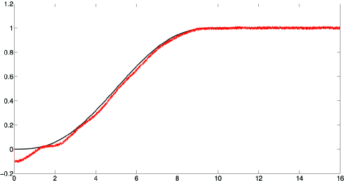
Figure 1: System output and reference

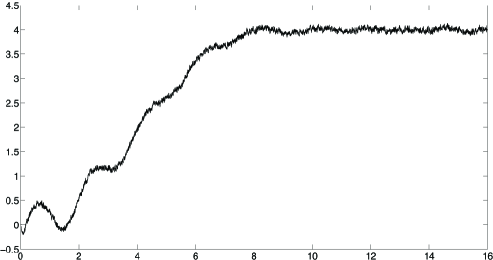
Figure 2: iPI control

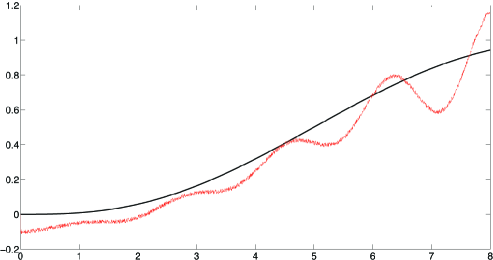
Figure 3: System output and reference

5 Numerical experiments

In the subsequent simulations the sampling time is $T_{e}=0.01\text{s}$. The corrupting noise is additive, normal, zero-mean, with a standard deviation equal in Sections 5.1 and 5.5 to $0.01$, and to $0.03$ elsewhere.

5.1 Control with a partially known system

5.1.1 A crude description

Consider the non-linear Duffing spring with friction:

$$m\ddot{y}=-{\mathcal{K}}(y)+{\mathcal{F}}(\dot{y})-d\dot{y}+F_{\tiny{\mbox{\rm ext}}}$$ (17)

where

• $y$ is the length of the spring,

• $m$ is a point mass,

• $F_{\tiny{\mbox{\rm ext}}}=u$ is the control variable,

• ${\mathcal{K}}(y)=k_{1}y+k_{3}y^{3}$ is the resulting force from the Hooke law and the Duffing cubic term,

• $d{\dot{y}}$ is a classic linear friction and ${\mathcal{F}}(\dot{y})$ a non-linear one. The term ${\mathcal{F}}(\dot{y})$ corresponds to the Tustin friction (Tustin (1947)) (see, also, Olsson, Aström, Canudas de Wit, Gäfvert & Lischinsky (1998)), which is rather violent with respect to the sign change of the speed (see Figure 4).

Set $m=0.5$, $k_{1}=3$. The partially known system

$$m\ddot{y}=k_{1}y+u$$

is flat, and $y$ is a flat output. It helps us to determine a suitable reference trajectory $y^{\star}$ and the corresponding nominal control variable $u^{\star}=m\ddot{y}^{\star}+k_{1}y^{\star}$. In the numerical simulations, we utilize $\hat{k}_{1}=2$, $d=1$, $k_{3}=2$, which are in fact unknown.

5.1.2 A PID controller

Set $u=u^{\star}+v$. Associate to $v$ a PID corrector for alleviating the tracking error $e=y-y^{\star}$ by imposing a denominator of the form $(s+1.5)^{3}$. The corresponding tuning gains are $k_{P}=1.375$, $k_{I}=1.6875$, $k_{D}=2.25$.

5.1.3 iPID

The main difference of the iPID is the following one: The presence of $F$ which is estimated in order to compensate the nonlinearities and the perturbations like frictions. For comparison purposes, its gains are the same as previously.

5.1.4 iP

We do not take any advantage of Equation (17). The error tracking dynamics is again given with a pole equal to $-1.5$, i.e., by the denominator $(s+1.5)$.

5.1.5 Numerical experiments

Figure 5 shows quite poor results with the PID of Section 5.1.2 . They become excellent with the iPID, and correct with iP. The practician might be right to prefer this last control synthesis

• where the implementation is immediate,

• if a most acute precision may be neglected.

(a) Tustin’s model

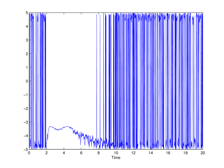
(b) Friction with the iPID

Figure 4: Model and time evolution of friction

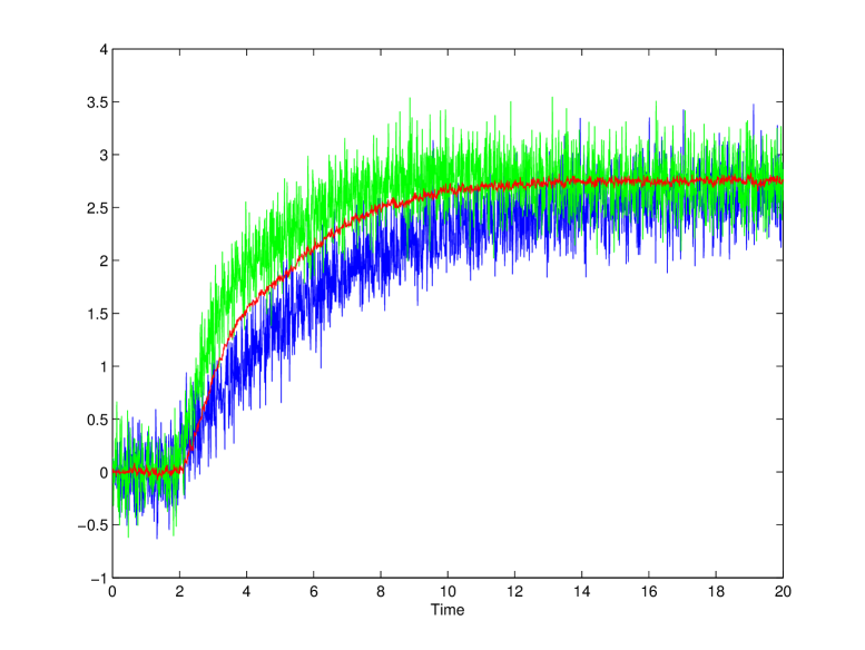
(a) Controls $F_{{\rm ext}}(t)$: PID(–, blue), iP(–, red), iPID(–, green)

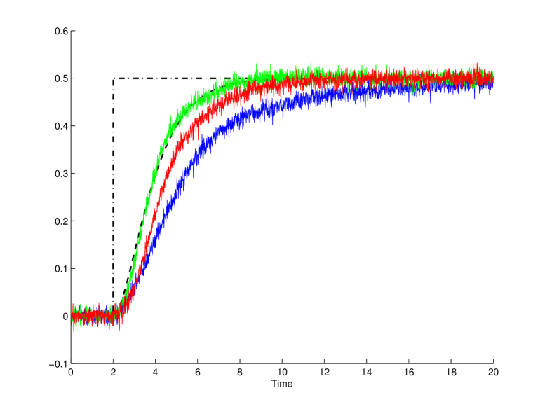
(b) Setpoint (- ., black), reference (- -, black), and output: PID(–, blue), iP(–, red), iPID(–, green)

Figure 5: Partially known system: comparisons

Remark 5.1

See also Villagra, d’Andréa-Novel, Choi, Fliess, & Mounier (2009) and Villagra & Balaguer (2011) for concrete examples related to guided vehicles.

5.2 Robustness with respect to system’s changes

The examples below demonstrate that if the system is changing, our intelligent controllers behave quite well without the need of any new calibration.

5.2.1 Scenario 1: the nominal case

The nominal system is defined by the transfer function

$$\frac{(s+2)^{2}}{(s+1)^{3}}$$ (18)

A tuning of a classic PID controller

$$u=k_{p}e+k_{i}\int e+k_{d}\dot{e}$$ (19)

where

• $e=y-y^{\ast}$ is the tracking error,

• $k_{p},k_{i},k_{d}\in\mathbb{R}$ are the gains,

yields via standard techniques (see, e.g., Åström & Hägglund (2006)) $k_{p}=1.8177$, $k_{i}=0.7755$, $k_{d}=0.1766$. A low-pass filter is moreover added to the derivative $\dot{e}$ in order to attenuate the corrupting noise. Our model-free approach utilizes the ultra-local model $\dot{y}=F+u$ and an iP (11) where $K_{P}=1.8177$. Figure 6 shows perhaps a slightly better behavior of the iP.

(a) Controls: PID(–, blue), iP(–, red)

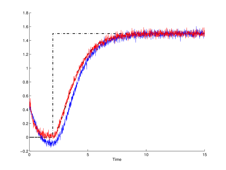
(b) Setpoint (- ., black), reference (- -, black), and outputs: PID(–, blue), iP(–, red)

Figure 6: Scenario 1: comparisons

5.2.2 Scenario 2: modifying the pole

A system change, aging for instance, might be seen by as new pole $-2.2$ in the transfer function (18) which becomes

$$\frac{(s+2)^{2}}{(s+2.2)^{3}}$$

As shown in Figure 7, without any new calibration the performances of the PID worsen whereas those of the iP remain excellent.

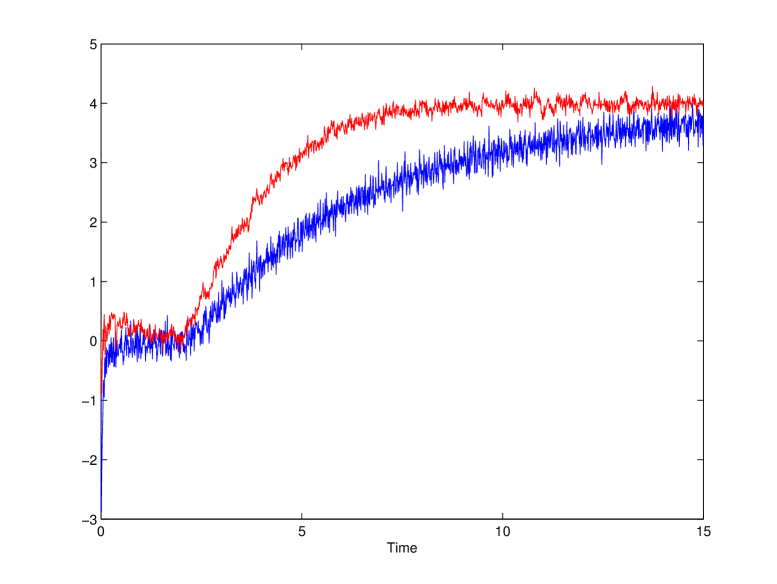
(a) Controls: PID(–, blue), iP(–, red)

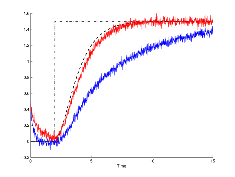
(b) Setpoint (- ., black), reference (- -, black), and outputs: PID(–, blue), iP(–, red)

Figure 7: Scenario 2: comparisons

5.2.3 Scenario 3: actuator’s fault

A power loss of the actuator occurs at time $t=8\text{s}$. It is simulated by dividing the control by $2$ at $t=8\text{s}$. Figure 8 shows an accommodation of the iP which is much faster than with the PID.

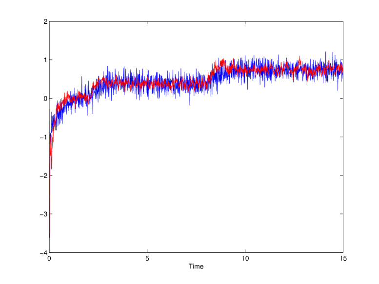
(a) Controls: PID(–, blue), iP(–, red)

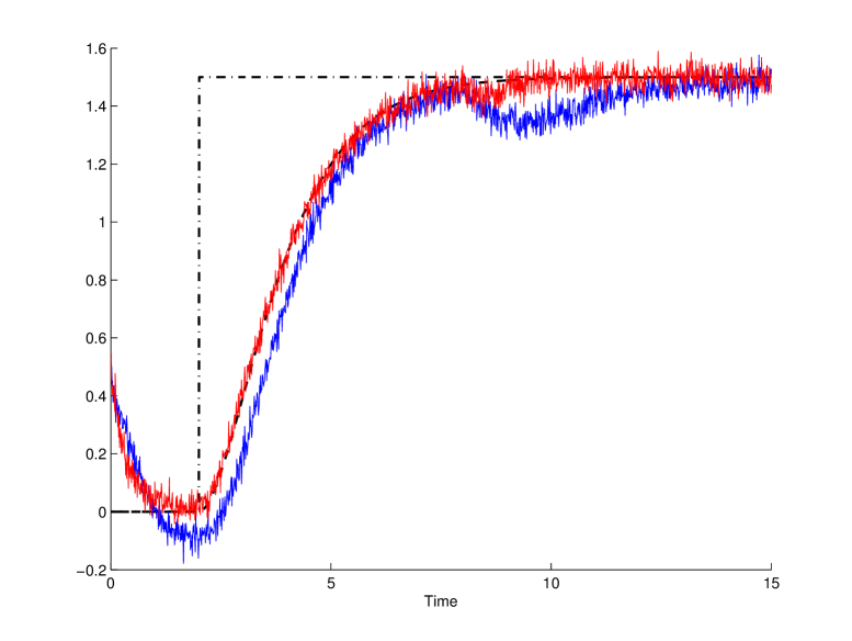
(b) Setpoint (- ., black), reference (- -, black), and outputs: PID(–, blue), iP(–, red)

Figure 8: Scenario 3: comparisons

Remark 5.2

Sections 5.2.2 and 5.2.3 may be understood as instances of fault accommodation, which contrarily to most of the existing literature are not model-based (see, also, Moussa Ali, Join & Hamelin (2012)). It is perhaps worth mentioning here that model-based fault diagnosis has also benefited from the estimation techniques summarized in Section 3 (see Fliess, Join & Sira-Ramírez (2004, 2008)).

5.3 A non-linear system

Take the following academic unstable non-linear system

$$\dot{y}-y=u^{3}$$

The clssic PID (19) is tuned with $k_{p}=2.2727$, $k_{i}=1.8769$, $k_{d}=0.1750$. The simulations depicted in Figure 9 shows a poor trajectory tracking for small values of the reference trajectory. The iP, which is related to the ultra-local model $\dot{y}=F+u$, corresponds to $K_{P}=2.2727$. Its excellent performances in the whole operating domain are also shown in Figure 9.

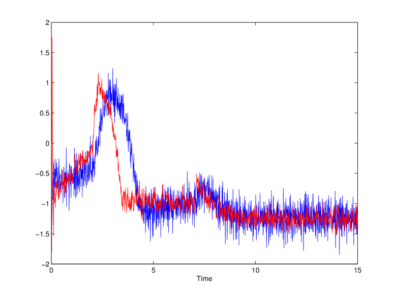
(a) Controls: PID(–, blue), iP(–, red)

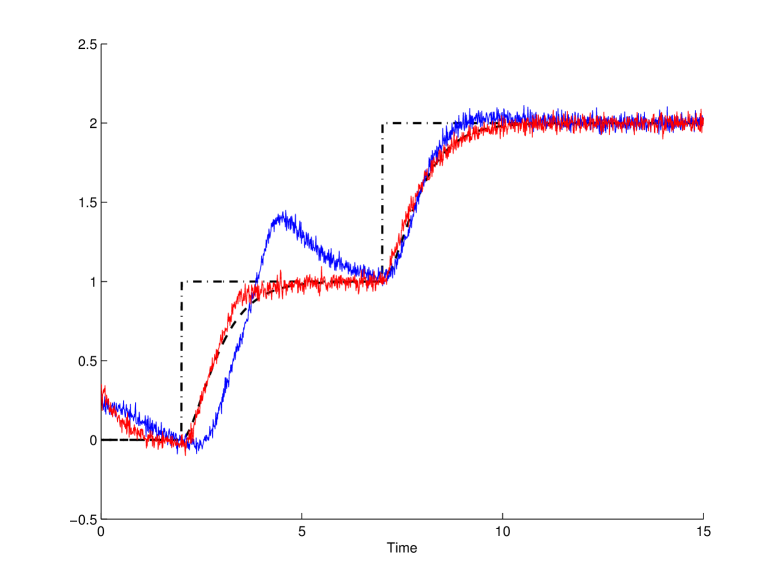
(b) Setpoint (- ., black), reference (- -, black), and outputs: PID(–, blue), iP(–, red)

Figure 9: Non-linear system: comparisons

5.4 Delay systems

Consider the system

$$\dot{y}(t)=y(t)+5y(t-\tau)+u$$

where moreover the delay $\tau$, $0\leq\tau\leq 5\text{s}$ is not assumed to be

• known,

• constant.

Set for the numerical simulations (see Figure 10)

$$\tau(t)=\tau(t-T_{e})+10T_{e}\text{sign}(N(t)),\quad\tau(0)=2.5\text{s}$$

where $N$ is a zero-mean Gaussian distribution with standard deviation $1$. An iP where $K_{P}=1$ is deduced from the ultra-local model $\dot{y}=F+u$. The results depicted in Figure 11 are quite satisfactory.

Figure 10: Delay function

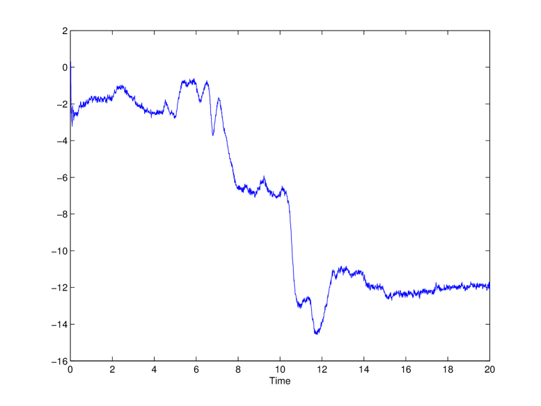
(a) Control

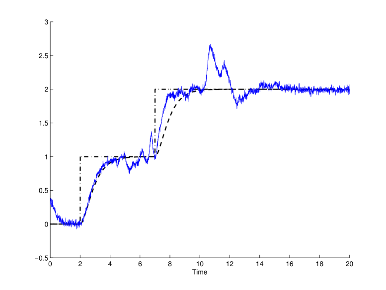
(b) Setpoint (- ., black), reference (- -, black), and output (–, blue)

Figure 11: Delay system: Model-free control

Remark 5.3

Extending the above control strategy to non-linear systems and to neutral systems is straightforward. It will not be developed here.

Remark 5.4

The delay appearing with the hydro-electric power plants studied by Join, Robert & Fliess (2010b) was taken into account via an empirical knowledge of the process. Some numerical tabulations were employed in order to get in some sense “rid” of the delay. Such a viewpoint might be the most realistic one in industry.

Remark 5.5

We only refer here to “physical” delays and not to the familiar approximation in engineering of “complex” systems via delays ones (see, e.g., Shinskey (1996)). Let us emphasize that this type of approximation is loosing its importance in our setting.

5.5 A one-dimensional semi-linear heat equation

The heat equation is certainly one of the most studied topic in mathematical physics. It would be pointless to review its corresponding huge bibliography even in the control domain, where many of the existing high-level control theories have been tested. Consider with Coron & Trélat (2004) the one-dimensional semi-linear heat equation

$$\frac{\partial w}{\partial t}=\frac{\partial^{2}w}{\partial x^{2}}+f(w)$$ (20)

where

• $0\leq x\leq L$,

• $w(t,0)=c$,

• $w(t,L)=u(t)$ is the control variable,

• $w(0,x)=sin(\pi x)+(u(0)-c)x+c$, where $c\in\mathbb{R}$ is a constant..

We want to obtain given time-dependent temperature at $x=x_{c}$. Consider the following scenarios:

1. $x_{c}=1/3L$, $f=0$, $c=0$,

2. $x_{c}=1/3L$, $f=0$, $c=0.5$,

3. $x_{c}=2/3L$, $f=0$, $c=0$,

4. $x_{c}=2/3L$, $f=y^{3}$, $c=0$.

The control synthesis is achieved thanks to the elementary one-dimensional ultra-local model

$$\dot{y}=F+10u$$

and the straightforward iP, where $K_{p}=10$. The four numerical simulations, displayed by Figures 12, 13, 14, and 15, are quite convincing.

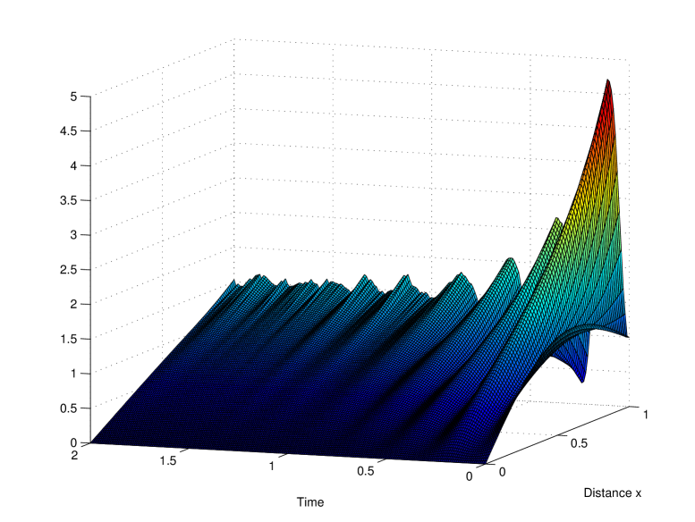
(a) Time evolution without measurement noise

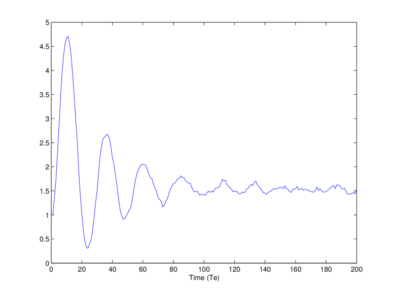
(b) Control $u(t)$

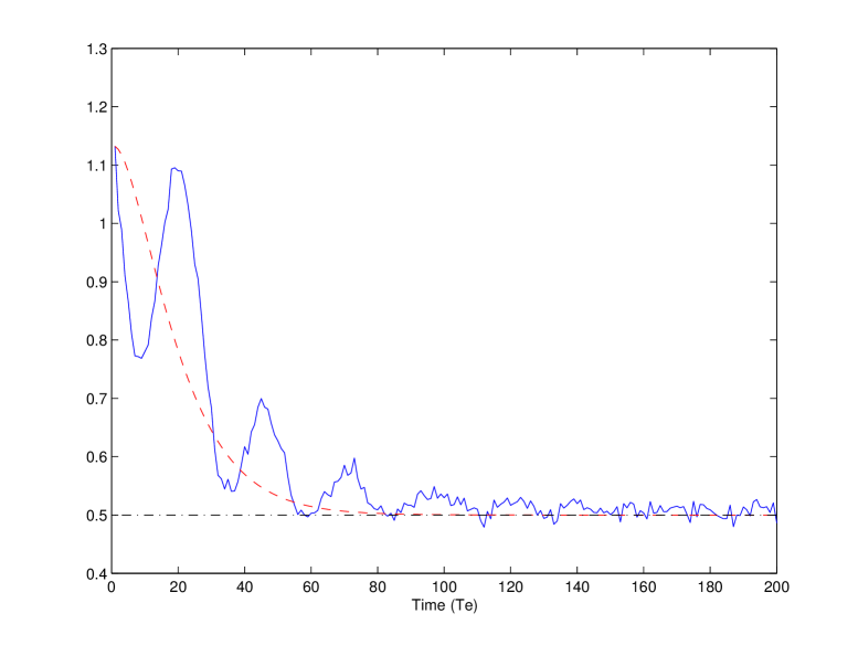
(c) Controlled heat at distance $x_{c}$ (–, blue), setpoint (- ., black), and reference (- -, red)

Figure 12: Heat equation: scenario 1

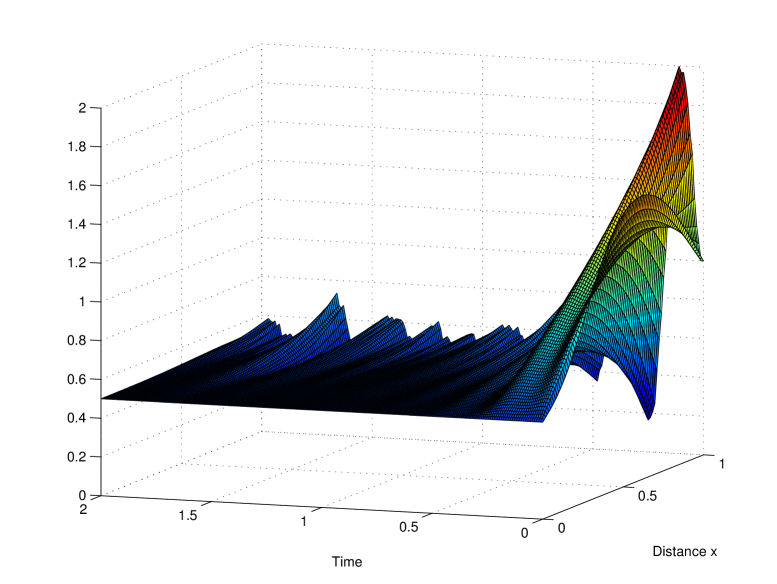
(a) Time evolution without measurement noise

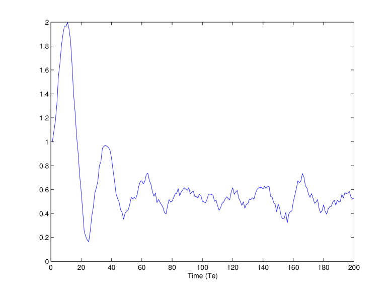
(b) Control $u(t)$

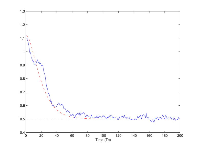
(c) Controlled heat at distance $x_{c}$ (–, blue), setpoint (- ., black), and reference (- -, red)

Figure 13: Heat equation: scenario 2

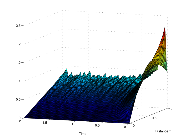
(a) Time evolution without measurement noise

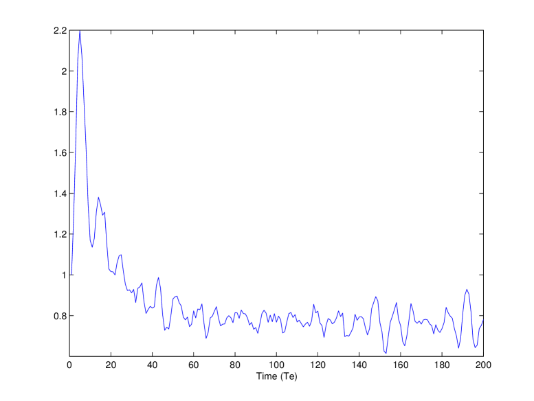
(b) Control $u(t)$

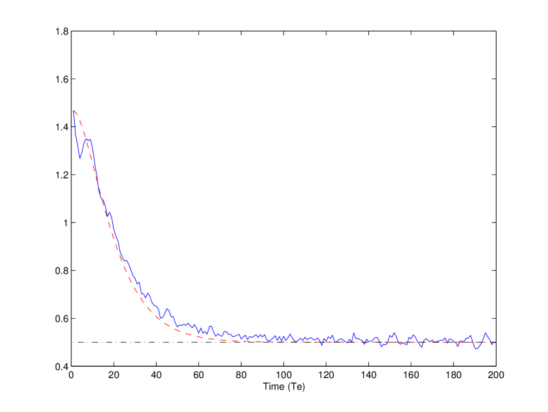
(c) Controlled heat at distance $x_{c}$ (–, blue), setpoint (- .,black), and reference (- -, red)

Figure 14: Heat equation: scenario 3

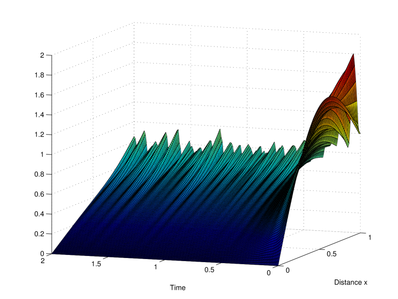
(a) Time evolution without measurement noise

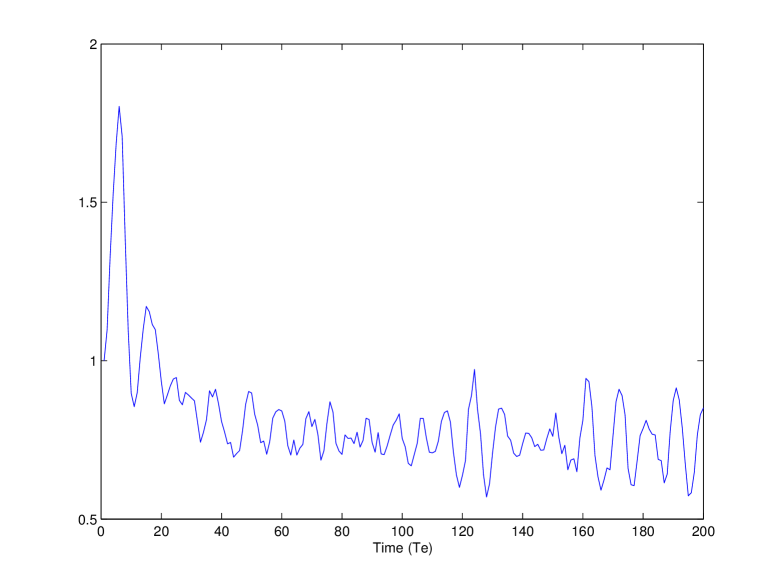
(b) Control $u(t)$

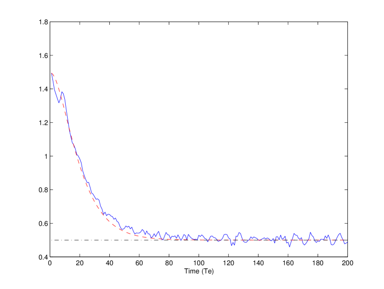
(c) Controlled heat at distance $x_{c}$ (–, blue), setpoint (- ., black), and reference (- -, red)

Figure 15: Heat equation: scenario 4

5.6 A peculiar non-minimum phase system

Consider the non-minimum phase system defined by the transfer function

$$\frac{(s-1)}{(s+1)(s+2)}$$ (21)

Utilize Equations (12) and (13). Set $\alpha=-\beta=10$, $K_{P}=3$ and $K_{I}=K_{II}=5$. Figure 16 displays good performances.

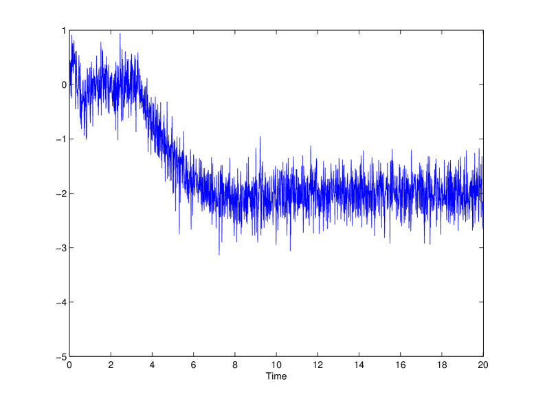
(a) Control

(b) Setpoint (- .,black) and Output (–,blue)

Figure 16: Non-minimum phase linear system: Model-free control

Remark 5.6

It is easy to check that the above calculations work only for a single unstable zero, like in Equation (21). Our approach cannot be extended to arbitrary non-minimum phase systems.

Remark 5.7

It is well known that the control synthesis of a non-minimum phase system is even a difficult task with a perfectly known mathematical model. Among the many solutions which have been suggested in the literature, let us mention a flatness-based output change (see Fliess & Marquez (2000); Fliess, Sira-Ramírez & Marquez (1998)). When a mathematical model is unknown or poorly known, the non-minimum phase character of an output cannot be deduced mathematically but only via a “bad” qualitative behavior of this output. Selecting a minimum phase output, i.e., an output with “good” qualitative properties, might be a more realistic alternative. It necessitates nevertheless an excellent “practical” knowledge of the plant behaviour.

6 Connections between classic and intelligent controllers

The results below connect classic PIDs to our intelligent controllers. They explain therefore why classic PIDs are used in rather arbitrary industrial situations thanks to a fine gain tuning, which might be quite difficult to achieve in practice.

6.1 PI and iP

6.1.1 A crude sampling of PIs

Consider the classic continuous-time PI controller

$$u(t)=k_{p}e(t)+k_{i}\int e(\tau)d\tau$$ (22)

A crude sampling of the integral $\int e(\tau)d\tau$ through a Riemann sum $I(t)$ leads to

$$\int e(\tau)d\tau\simeq I(t)=I(t-h)+he(t)$$

where $h$ is the sampling interval. The corresponding discrete form of Equation (22) reads:

$$u(t)=k_{p}e(t)+k_{i}I(t)=k_{p}e(t)+k_{i}I(t-h)+k_{i}he(t)$$

Combining the above equation with

$$u(t-h)=k_{p}e(t-h)+k_{i}I(t-h)$$

yields

$$u(t)=u(t-h)+k_{p}\left(e(t)-e(t-h)\right)+k_{i}he(t)$$ (23)

Remark 6.1

A trivial sampling of the “velocity form” of Equation (22)

$$\dot{u}(t)=k_{p}\dot{e}(t)+k_{i}e(t)$$

yields

$$\dfrac{u(t)-u(t-h)}{h}=k_{p}\left(\dfrac{e(t)-e(t-h)}{h}\right)+k_{i}e(t)$$

which is equivalent to Equation (23).

6.1.2 Sampling iPs

Utilize, if $\nu=1$, the iP, which may be rewritten as

$$u(t)=\frac{{\dot{y}}^{\ast}(t)-F+K_{P}e(t)}{\alpha}$$

Replace $F$ by ${\dot{y}}(t)-\alpha u(t-h)$ and therefore by

$$\frac{y(t)-y(t-h)}{h}-\alpha u(t-h)$$

It yields

$$u(t)=u(t-h)-\frac{e(t)-e(t-h)}{h\alpha}+\dfrac{K_{P}}{\alpha}\,e(t)$$ (24)

6.1.3 Comparison

FACT.- Equations (23) and (24) become identical if we set

$$k_{p} =-\dfrac{1}{\alpha h},\quad k_{i}=\dfrac{K_{P}}{\alpha h}$$ (25)

Remark 6.2

It should be emphasized that the above property, defined by Equations (25), does not hold for continuous-time PIs and iPs. This equivalence is strictly related to time sampling, i.e., to computer implementation, as demonstrated by taking $h\downarrow 0$ in Equations (25).

6.2 PID and iPD

Extending the calculations of Section 6.1 is quite obvious. The velocity form of the PID

$$u(t)=k_{p}e(t)+k_{i}\int e(\tau)d\tau+k_{d}\dot{e}$$

reads $\dot{u}(t)=k_{p}{\dot{e}}(t)+k_{i}e(t)+k_{d}{\ddot{e}}(t)$. It yields the obvious sampling

$$u(t)=u(t-h)+k_{p}h{\dot{e}}(t)+k_{i}he(t)+k_{d}h{\ddot{e}}(t)$$ (26)

$\nu=2$ on the other hand, Equation yields $u(t)=\dfrac{1}{\alpha}\left({\ddot{y}}^{\ast}(t)-F+K_{P}e(t)+K_{D}{\dot{e}}(t)\right)$. From the computer implementation $F=\ddot{y}(t)-\alpha u(t-h)$, we derive

$$u(t)=u(t-h)-\dfrac{1}{\alpha}{\ddot{e}}(t)+\dfrac{K_{P}}{\alpha}e(t)+\dfrac{K_{D}}{\alpha}{\dot{e}}(t)$$ (27)

FACT.- Equations (26) and (27) become identical if we set

$$k_{p}=\dfrac{K_{D}}{\alpha h},\quad k_{i}=\dfrac{K_{P}}{\alpha h},\quad k_{d}=-\dfrac{1}{\alpha h}$$ (28)

6.3 iPI and iPID

Equation (27) becomes with the iPID

$$u(t)=u(t-h)-\dfrac{1}{\alpha}{\ddot{e}}(t)+\dfrac{K_{P}}{\alpha}e(t)+\dfrac{K_{I}}{\alpha}\int e+\dfrac{K_{D}}{\alpha}{\dot{e}}(t)$$ (29)

Introduce the PI²D controller

$$u(t)=k_{p}e(t)+k_{i}\int e(\tau)d\tau+k_{ii}\int\!\!\!\!\int ed\tau d\sigma+k_{d}\dot{e}(t)$$

The double integral, which appears there, seems to be quite uncommon in control engineering. To its velocity form ${\dot{u}}(t)=k_{p}\dot{e}(t)+k_{i}e+k_{ii}\int ed\tau+k_{d}\ddot{e}(t)$ corresponds the sampling

$$u(t)=u(t-h)+k_{p}h\dot{e}(t)+k_{i}he+k_{ii}h\int ed\tau+k_{d}h\ddot{e}(t)$$

which is identical to Equation (29) if one sets

$$k_{p} =\dfrac{K_{D}}{\alpha h},\quad k_{i}=\dfrac{K_{P}}{\alpha h},\quad k_{ii}=\dfrac{K_{I}}{\alpha h},\quad k_{d}=-\dfrac{1}{\alpha h}$$ (30)

The connection between iPIs and PI²s follows at once.

6.4 Table of correspondence

The previous calculations yield the following correspondence (Table 1) between the gains of our various controllers:

		iP	iPD	iPI	iPID
PI	$k_{p}$	$-1/\alpha h$
	$k_{i}$	$K_{P}/\alpha h$
PID	$k_{p}$		$K_{D}/\alpha h$
	$k_{i}$		$K_{P}/\alpha h$
	$k_{d}$		$-1/\alpha h$
PI2	$k_{p}$			$-1/\alpha h$
	$k_{i}$			$K_{P}/\alpha h$
	$k_{ii}$			$K_{I}/\alpha h$
PI2D	$k_{p}$				$K_{D}/\alpha h$
	$k_{i}$				$K_{P}/\alpha h$
	$k_{ii}$				$K_{I}/\alpha h$
	$k_{d}$				$-1/\alpha h$

Table 1: Correspondence between the gains of sampled classic and intelligent controllers.

Remark 6.3

Due to the form of Equation (22), it should be noticed that the tuning gains of the classic regulators ought to be negative.

7 Conclusion

Several theoretical questions remain of course open. Let us mention some of them, which appear today to be most important:

• The fact that multivariable systems were not studied here is due to a lack until now of concrete case-studies. They should therefore be examined more closely.

• Even if some delay and/or non-minimum phase examples were already successfully treated (see Sections 5.4, 5.6, and (Andary, Chemori, Benoit & Sallantin (2012); Join, Robert & Fliess (2010b); Riachy, Fliess, Join & Barbot (2010))), a general understanding is still missing, like, to the best of our knowledge, with any other recent setting (see, e.g., Åström & Hägglund (2006); O’Dwyer (2009), and Xu, Li & Wang (2012)). We believe as advocated in Remarks 5.4 and 5.7 that

  • looking for a purely mathematical solution might be misleading,

  • taking advantage on the other hand of a “good” empirical understanding of the plant might lead to a more realistic track.

It goes without saying that comparisons with existing approaches should be further explored. It has already been done with

• classic PIDs here, and by Gédouin, Delaleau, Bourgeot, Join, Arab-Chirani & Calloch (2011); Milanes, Villagra, Perez & Gonzalez (2012) for some active spring and vehicles,

• some aspects of sliding modes by Riachy, Fliess & Join (2011),

• fuzzy control for some vehicles by Milanes, Villagra, Perez & Gonzalez (2012); Villagra & Balaguer (2011).

Those comparisons were until now always favourable to our setting.

If model-free control and the corresponding intelligent controllers are further reinforced, especially by numerous fruitful applications, the consequences on the future development and teaching (see, e.g., the excellent textbook by Åström & Murray (2008)) of control theory might be dramatic:

• Questions on the structure and on the parameter identification of linear and nonlinear systems might loose their importance if the need of a “good” mathematical modeling is diminishing.

• Many effort on robustness issues with respect to a “poor” modeling and/or to disturbances may be viewed as obsolete and therefore less important. As a matter of fact those issues disappear to a large extent thanks to the continuously updated numerical values of $F$ in Equation (1).

Another question, which was already raised by Abouaïssa, Fliess, Iordanova & Join (2012), should be emphasized. Our model-free control strategy yields a straightforward regulation of industrial plants whereas the corresponding digital simulations need a reasonably accurate mathematical model in order to feed the computers. Advanced parameter identification and numerical analysis techniques might then be necessary tools (see, e.g., Join, Robert & Fliess (2010b); Abouaïssa, Fliess, Iordanova & Join (2012)). This dichotomy between elementary control implementations and intricate computer simulations seems to the best of our knowledge to have been ignored until today. It should certainly be further dissected as a fundamental epistemological matter in engineering and, perhaps also, in other fields.

Appendix A An approximation property

A.1 Functionals

We restrict ourselves to a SISO system, i.e., to a system with a single control variable $u$ and a single output $y$. Even without knowing any “good” mathematical model we may assume that the system corresponds to a causal, or non-anticipative, functional, i.e., for any time instant $t>0$,

$$y(t)=\mathcal{F}\left(u(\tau)\leavevmode\nobreak\ |\leavevmode\nobreak\ 0\leq\tau\leq t\right)$$ (31)

where $\mathcal{F}$ depends on

• the past and the present, and not on the future,

• various perturbations,

• initial conditions at $t=0$.

Example A.1

A popular representation of rather arbitrary nonlinear systems in engineering is provided by Volterra series (see, e.g., Barrett (1963), Rugh (1981) and Lamnabhi-Lagarrigue (1995)). Such a series may be defined by

$$y(t)= h_{0}(t)+\int_{0}^{t}h_{1}(t,\tau)u(\tau)d\tau+$$

$$\int_{0}^{t}\int_{0}^{t}h_{2}(t,\tau_{2},\tau_{1})u(\tau_{2})u(\tau_{1})d\tau_{2}d\tau_{1}+\dots$$

$$\int_{0}^{t}\dots\int_{0}^{t}h_{\nu}(t,\tau_{\nu},\dots\tau_{1})u(\tau_{\nu})\dots u(\tau_{1})d\tau_{\nu}\dots d\tau_{1}$$

$$+\dots$$

Solutions of quite arbitrary differential equations may be expressed as Volterra series.

A.2 The Stone-Weierstraß theorem

Let

• $\mathcal{I}\subset[0,+\infty[$ be a compact subset,

• $\mathcal{C}\subset C^{0}(\mathcal{I})$ be a compact subset, where $C^{0}(\mathcal{I})$ is the space of continuous functions $\mathcal{I}\rightarrow\mathbb{R}$, which is equipped with the topology of uniform convergence.

Consider the Banach $\mathbb{R}$-algebra $\mathfrak{S}$ of continuous causal functionals (31) $\mathcal{I}\times\mathcal{C}\rightarrow\mathbb{R}$. If a subalgebra contains a non-zero constant element and separates points in $\mathcal{I}\times\mathcal{C}$, then it is dense in $\mathfrak{S}$ according to the Stone-Weierstraß theorem (see, e.g., the excellent textbooks by Choquet (2000) and Rudin (1967)).

A.3 Algebraic differential equations

Let $\mathfrak{A}\subset\mathfrak{S}$ be the set of functionals which satisfy an algebraic differential equation of the form

$$E(y,\dot{y},\dots,y^{(a)},u,\dot{u},\dots,u^{(b)})=0$$ (32)

where $E$ is a polynomial function of its arguments with real coefficients. Satisfying Equation (32) is equivalent saying that $y$ is differential algebraic over the differential field $\mathbb{R}\langle u\rangle$.

Remark A.1

Remind that a differential field (see, e.g., the two following books by Chambert-Loir (2005) and Kolchin (1973), and the papers by Delaleau (2002), Fliess, Join & Sira-Ramírez (2008) and Fliess, Lévine, Martin & Rouchon (1995)) is a commutative field which is equipped with a derivation. A typical element of $\mathbb{R}\langle u\rangle$ is a rational function of $u$, $\dot{u}$, …, $u^{(\nu)}$, …, with real coefficients.

It is known (Kolchin (1973)) that the sum and the product of two elements which are differentially algebraic over $\mathbb{R}\langle u\rangle$ is again differentially algebraic over $\mathbb{R}\langle u\rangle$. It is obvious moreover that any constant element, which satisfies $\dot{y}=0$, belongs to $\mathfrak{A}$.

Take two distinct points $(\tau,u),(\tau^{\prime},u^{\prime})\in\mathcal{I}\times\mathcal{C}$. If $\tau\neq\tau^{\prime}$, then $y=t$, which satisfies $\dot{y}=1$, separates the two points. If $\tau=\tau^{\prime}$, then assume that $u\neq u$ on the interval $[0,\tau]$. It follows from Lerch’s theorem (Lerch (1903)) (see, also, Mikusiński (1983)) that there exists a non-negative integer $\nu$ such that

$$\int_{0}^{t}\sigma^{\nu}u(\sigma)d\sigma\neq\int_{0}^{t}\sigma^{\nu}u^{\prime}(\sigma)d\sigma$$

The classic Cauchy formula demonstrates the existence of a non-negative integer $\nu$ such that $y$, which satisfies $y^{(\nu)}=u$, separates $(\tau,u)$, $(\tau,u^{\prime})$.

This proof, which mimics to some extent Fliess (1976, 1981) (see, also, Sussmann (1976)), shows that $\mathfrak{A}$ is dense in $\mathfrak{S}$.

Appendix B Justification of the ultra-local model

Assume that our SISO system is “well” approximated by a system described by Equation (32). Let $\nu$ be a non-negative integer such that

$$\frac{\partial E}{\partial y^{(\nu)}}\not\equiv 0$$

The implicit function theorem yields then locally

$$y^{(\nu)}=\mathcal{E}(y,\dot{y},\dots,y^{(\nu-1)},y^{(\nu+1)},\dots,y^{(a)},u,\dot{u},\dots,u^{(b)})$$

It may be rewritten as Equation (1).

References

- Abouaïssa, Fliess, Iordanova & Join (2012) Abouaïssa, H., Fliess, M., Iordanova, V. and Join, C. (2012), ‘Freeway ramp metering control made easy and efficient’, in 13th IFAC Symp. Control Transportation Systems, Sofia. Available at http://hal.archives-ouvertes.fr/hal-00711847/en/
- Andary, Chemori, Benoit & Sallantin (2012) Andary, S., Chemori, A., Benoit, M., and Sallantin J. (2012), ‘A dual model-free control of underactuated mechanical systems – Application to the inertia wheel inverted pendulum with real-time experiments’, in Amer. Control Conf., Montréal.
-
d’Andréa-Novel, Boussard, Fliess, el Hamzaoui, Mounier & Steux (2010)
d’Andréa-Novel, B., Boussard, C., Fliess, M., el Hamzaoui, O.,
Mounier, H., and Steux, B. (2010), ‘Commande sans modèle de vitesse
longitudinale d’un véhicule électrique’, in 6e Conf.
Internat. Francoph. Automatique, Nancy. Available at
http://hal.archives-ouvertes.fr/inria-00463865/en/ - d’Andréa-Novel, Boussard, Fliess, Join, Mounier & Steux (2010) d’Andréa-Novel, B., Fliess, M., Join, C., Mounier, H., and Steux (2010), ‘A mathematical explanation via “intelligent” PID controllers of the strange ubiquity of PIDs’, in 18th Medit. Conf. Control Automat., Marrakech. Available at http//hal.archives-ouvertes.fr/inria-00480293/en/
- Åström & Hägglund (2006) Åström, K.J., and Hägglund, T. (2006), Advanced PID Control, Instrument Soc. Amer..
- Åström, Hang, Persson & Ho (1992) Åström, K.J., Hang, C.C., Persson, P., and Ho, W.K. (1992), ‘Towards intelligent PID control’, Automatica, 28, 1–9.
- Åström & Murray (2008) Åström, K.J., and Murray, R.M. (2008), Feedback Systems: An Introduction for Scientists and Engineers, Princeton University Press.
- Barrett (1963) Barrett, J.F. (1963), ‘The use of functionals in the analysis of non-linear physical systems’, J. Electron. Control, 15, 567–615.
- Bilal Kadri (2009) Bilal Kadri, M. (2009), Model Free Adaptive Fuzzy Control: Beginners Approach, VDM Verlag.
- Chambert-Loir (2005) Chambert-Loir, A. (2005), Algèbre corporelle, Éditions École Polytechnique. English translation (2005): A Field Guide to Algebra, Springer.
- Chang, Gao & Gu (2011) Chang, Y., Gao, B., and Gu, K. (2011), ‘A model-free adaptive control to a blood pump based on heart rate’, Amer. Soc. Artificial Internal Organs J., 57, 262–267.
- Chang & Jung (2009) Chang, P.H., and Jung, P.H. (2009), ‘A systematic method for gain selection of robust PID control for nonlinear plants of second-order controller canonical form’, IEEE Trans. Contr. Systems Technology, 17, 473–483.
- Choi, d’Andréa-Novel, Fliess, Mounier & Villagra (2009) Choi, S., d’Andréa-Novel, B., Fliess, M., Mounier, H., and Villagra, J. (2009), ‘Model-free control of automotive engine and brake for Stop-and-Go scenarios’, in 10th Europ. Control Conf., Budapest. Available at http://hal.archives-ouvertes.fr/inria-00395393/en/
- Choquet (2000) Choquet, G. (2000), Cours de topologie, Dunod.
- Coron & Trélat (2004) Coron, J.-M., and Trélat, E. (2004), ‘Global steady-state controllability of one-dimensional semilinear heat equations’, SIAM J. Control Optimiz., 43, 549–569.
- Delaleau (2002) Delaleau, E. (2002), ‘Algèbre différentielle’, in ed. J.-P. Richard, Mathématiques pour les systèmes dynamiques, vol. 2, chapter 6, pp. 245–268, Hermes.
- De Miras, Riachy, Fliess, Join & Bonnet (2012) De Miras, J., Riachy, S., Fliess, M., Join, C., and Bonnet, S. (2012), ‘Vers une commande sans modèle d’un palier magnétique’, in 7e Conf. Internat. Francoph. Automatique, Grenoble. Available at http://hal.archives-ouvertes.fr/hal-00682762/en/
- Fliess (1976) Fliess, M. (1976), ‘Un outil algébrique: les séries formelles non commutatives’, in eds G. Marchesini and S.K. Mitter, Mathematical System Theory, Lect. Notes Econom. Math. Syst., Vol. 131, pp. 122–148, Springer.
- Fliess (1981) Fliess, M. (1981), ‘Fonctionnelles causales non linéaires et indéterminées non commutatives’, Bull. Soc. Math. France, 109, 3–40.
- Fliess (2006) Fliess, M. (2006), ‘Analyse non standard du bruit’, C.R. Acad. Sci. Paris Ser. I, 342, 797–802.
-
Fliess & Join (2008a)
Fliess, M., and Join, C. (2008a), ‘Intelligent PID controllers’, in
16th Medit. Conf. Control Automation, Ajaccio. Available at
http://hal.archives-ouvertes.fr/inria-00273279/en/ -
Fliess & Join (2008b)
Fliess, M., and Join, C. (2008b), ‘Commande sans modèle et commande à
modèle restreint’, e-STA, 5 (n∘ 4): 1–23. Available
at
http://hal.archives-ouvertes.fr/inria-00288107/en/ -
Fliess & Join (2009)
Fliess, M., and Join, C. (2009), ‘Model-free control and intelligent
PID controllers: towards a possible trivialization of nonlinear
control?’, in 15th IFAC Symp. System Identif.,
Saint-Malo. Available at
http://hal.archives-ouvertes.fr/inria-00372325/en/ - Fliess, Join & Mboup (2010) Fliess, M., Join, C., Mboup, M. (2010), ‘Algebraic change-point detection’, Appl. Algebra Engin. Communic. Computing, 21, 131–143.
-
Fliess, Join, Mboup & Sira-Ramírez (2006)
Fliess, M., Join, C., Mboup, M., and Sira-Ramírez, H. (2006), ‘Vers
une commande multivariable sans modèle’, in 4e Conf. Int.
Francoph. Automatique, Bordeaux. Available at
http://hal.archives-ouvertes.fr/inria-00001139/en/ -
Fliess, Join & Riachy (2011a)
Fliess, M., Join, C., and Riachy, S. (2011a), ‘Revisiting some practical issues in the implementation of model-free control’, in
18th IFAC World Congress, Milan. Available at
http://hal.archives-ouvertes.fr/hal-00576955/en/ -
Fliess, Join & Riachy (2011b)
Fliess, M., Join, C., and Riachy, S. (2011b), ‘Rien de plus utile
qu’une bonne théorie: la commande sans modèle’, in
Journées Nationales/Journées Doctorales Modélisation Analyse Conduite Systèmes, Marseille. Available at
http://hal.archives-ouvertes.fr/hal-00581109/en/ - Fliess, Join & Sira-Ramírez (2004) Fliess, M., Join, C., and Sira-Ramírez, H. (2004), ‘Robust residual generation for linear fault diagnosis: an algebraic setting with examples’, Int. J. Control, 77, 1223–1242.
- Fliess, Join & Sira-Ramírez (2006) Fliess, M., Join, C., and Sira-Ramírez, H. (2006), ‘Complex continuous nonlinear systems: Their black box identification and their control’, in 14th Symp. Syst. Identif., Newcastle, Australia. Available at http://hal.archives-ouvertes.fr/inria-00000824
-
Fliess, Join & Sira-Ramírez (2008)
Fliess, M., Join, C., and Sira-Ramírez, H. (2008), ‘Non-linear
estimation is easy’, Int. J. Modelling Identification
Control, 4, 12–27. Available at
http://hal.archives-ouvertes.fr/inria-00158855/en/ - Fliess, Lévine, Martin & Rouchon (1995) Fliess, M., Lévine, J., Martin, P., and Rouchon, P. (1995), ‘Flatness and defect of non-linear systems: introductory theory and examples’, Int. J. Control, 61, 1327–1361.
- Fliess & Marquez (2000) Fliess M., and Marquez, R. (2002), ‘Continuous-time linear predictive control and flatness: a module-theoretic setting with examples’, Int. J. Control, 73, 606-623.
- Fliess, Marquez, Delaleau & Sira-Ramírez (2002) Fliess, M., Marquez, R., Delaleau, E. and Sira-Ramírez, H.(2002), ‘Correcteurs proportionnels-intégraux généralisés’, ESAIM Control Optimiz. Calc. Variat., 7, 23–41.
- Fliess & Sira-Ramírez (2003) Fliess, M., and Sira-Ramírez, H. (2003), ‘An algebraic framework for linear identification’, ESAIM Control Optimiz. Calc. Variat., 9, 151–168.
- Fliess & Sira-Ramírez (2008) Fliess, M., and Sira-Ramírez, H. (2008), ‘Closed-loop parametric identification for continuous-time linear systems via new algebraic techniques’, in eds. H. Garnier and L. Wang, Identification of Continuous-time Models from Sampled Data, Springer, pp. 362–391.
- Fliess, Sira-Ramírez & Marquez (1998) Fliess, M., Sira-Ramírez, H., and Marquez, R. (1998), ‘Regulation of non-minimum phase outputs: a flatness based approach’, in ed. D. Normand-Cyrot, Perspectives in Control –Theory and Applications: a Tribute to Ioan Doré Landau, Springer, pp. 143–164.
- Formentin, de Filippi, Corno, Tanelli & Savaresi (2013) Formentin, S., de Filippi, P., Corno, M., Tanelli, M., and Savaresi, S. (2013), ‘Data-driven design of braking control systems’, IEEE Trans. Control Syst. Techno., 21, 186-193.
- Formentin, de Filippi, Tanelli & Savaresi (2010) Formentin, S., de Filippi, P., Tanelli, M., and Savaresi, S. (2010), ‘Model-free control for active braking systems in sport motorcycles’, in 8th IFAC Symp. Nonlinear Control Systems, Bologne.
- Gédouin, Delaleau, Bourgeot, Join, Arab-Chirani & Calloch (2011) Gédouin, P.-A., Delaleau, E., Bourgeot, J.-M., Join, C., Arab-Chirani, S., and Calloch, S. (2011), ‘Experimental comparison of classical pid and model-free control: position control of a shape memory alloy active spring’, Control Eng. Practice, 19, 433–441.
- Gehring, Knüppel, Rudolph & Woittennek (2012) Gehring, N., Knüppel, T., Rudolph, J., and Woittennek, F. (2012), ‘Algebraische Methoden zur Parameteridentifikation für das schwere Seil’, at - Automat., 60, 514–521.
- Godement (1998) Godement, R. (1998), Analyse mathématique II, Springer.
- Hahn & Oldham (2012) Hahn, B., and Oldham, K.R. (2012), ‘A model-free ON-OFF iterative adaptive controller based on stochastic approximation’, IEEE Trans. Control Systems Techno., 20, 196–204.
- Han (2009) Han, J. (2009), ‘From PID to active disturbance rejection control’, IEEE Trans. Indust. Electron., 56, 900–906.
- Hong-wei, Rong-min & Hui-xing (2011) Hong-wei, L., Rong-min, C., and Hui-xing, Z. (2011), ‘Application research on model-free control strategy of permanent magnetism linear synchronous motors’, in Internat. Conf. Electrical Machines Systems, Beijing.
-
Join, Masse & Fliess (2008)
Join, C., Masse, J., and Fliess, M. (2008), ‘Étude préliminaire
d’une commande sans modèle pour papillon de moteur’, J. Europ.
Syst. Automat., 42, 337–354. Available at
http://hal.archives-ouvertes.fr/inria-00187327/en/ - Join, Robert & Fliess (2010a) Join, C., Robert, G. and Fliess, M. (2010a), ‘Model-free based water level control for hydroelectric power plants’, in IFAC Conf. Control Method. Technologies Energy Efficiency, Vilamoura. Available at http://hal.archives-ouvertes.fr/inria-00458042/en/
- Join, Robert & Fliess (2010b) Join, C., Robert, G. and Fliess, M. (2010b), ‘Vers une commande sans modèle pour aménagements hydroélectriques en cascade’, in 6e Conf. Internat. Francoph. Automat., Nancy. Available at http://hal.archives-ouvertes.fr/inria-00460912/en/
- Keel & Bhattacharyya (2008) Keel, L.H., and Bhattacharyya, S.P. (2008), ‘Controller synthesis free of analytical models: Three term controllers’, IEEE Trans. Automat. Control, 53, 1353–1369.
- Killingsworth & Krstic (2006) Killingsworth, N.J., Krstic, M. (2006), ‘PID tuning using extremum seeking: online, model-free performance optimization’, IEEE Control Syst., 26, 70–79.
- Kolchin (1973) Kolchin, E.R. (1973), Differential Algebra and Algebraic Groups, Academic Press.
-
Lafont, Pessel, Balmat & Fliess (2013)
Lafont, F., Pessel, N., Balmat, J.-F, and Fliess, M. (2013), ‘On the model-free control of an experimental greenhouse’, in
Int. Conf. Modeling Simulation Control , San Francisco. Available at
http://hal.archives-ouvertes.fr/hal-00831598/en/ - Lamnabhi-Lagarrigue (1995) Lamnabhi-Lagarrigue, F. (1995), ‘Volterra and Fliess series expansions for nonlinear systems’, in ed. W.S. Levine, The Control Handbook, CRC Press, pp. 879–888.
- Lerch (1903) Lerch, M. (1903), ‘Sur un point de la théorie des fonctions génératrices d’Abel’, Acta Math., 27, 339–352.
- Lévine (2009) Lévine, J. (2009), Analysis and Control of Nonlinear Systems – A flatness-based approach, Springer.
- Liu, Gibaru & Perruquetti (2011) Liu, D.Y., Gibaru, O., Perruquetti, W. (2011), ‘Error analysis of Jacobi derivative estimators for noisy signals’, Numer. Algor., 58, 53–83.
- Lobry & Sari (2008) Lobry, C., Sari, T. (2008), ‘Nonstandard analysis and representation of reality’, Int. J. Control, 81, 519–536.
- Malis & Chaumette (2002) Malis, E., Chaumette, F. (2002), ‘Theoretical improvements in the stability analysis of a new class of model-free visual servoing methods’, IEEE Trans. Robotics, 18, 176–186.
- Mboup, Join & Fliess (2009) Mboup, M., Join, C., and Fliess, M. (2009), ‘Numerical differentiation with annihilators in noisy environment’, Numer. Algor., 50, 439–467.
-
Menhour, d’Andréa-Novel, Boussard, Fliess & Mounier (2011)
Menhour, L., d’Andréa-Novel, B., Boussard, C., Fliess, M., Mounier, H. (2011),
‘Algebraic nonlinear estimation and flatness-based lateral/longitudinal control for automotive vehicles’, in
14th Int. IEEE Conf. Intellig. Transport. Syst., Washington. Available at
http://hal.archives-ouvertes.fr/hal-00611950/en/ -
Michel, Join, Fliess, Sicard & Chériti (2010)
Michel, L., Join, C., Fliess, M., Sicard, P., and Chériti, A.
(2010), ‘Model-free control of dc/dc converters’, in IEEE
Compel, Boulder. Available at
http://hal.archives-ouvertes.fr/inria-00495776/en/ - Mikusiński (1983) Mikusiński, J. (1983), Operational Calculus, vol. 1, PWN & Pergamon Press.
- Milanes, Villagra, Perez & Gonzalez (2012) Milanes, V., Villagra, J., Perez, J., Gonzalez, C. (2012), ‘Low-speed longitudinal controllers for mass-produced cars: A comparative study’, IEEE Trans. Industrial Electronics, 59, 620–628.
- Morales, Feliu & Sira-Ramírez (2011) Morales, R., Feliu, V., and H. Sira-Ramírez, H. (2011), ‘Nonlinear control for magnetic levitation systems based on fast online algebraic identification of the input gain’, IEEE Trans. Control Syst. Techno., 19, 757–771.
- Morales, Nieto, Trapero, Chichamo & Pintado (2011) Morales, A., Nieto, A., Trapero J.R., Chicharro, J., and Pintado, P. (2011), ‘An adaptive pneumatic suspension based on the estimation of the excitation frequency’, J. Sound Vibration, 330, 1891–1903.
- Morales & Sira-Ramírez (2011) Morales, R., and Sira-Ramírez, H. (2010), ‘Trajectory tracking for the magnetic ball levitation system via exact feedforward linearisation and GPI control’, Int. J. Control, 83, 1155-1166.
- Moussa Ali, Join & Hamelin (2012) Moussa Ali, A., Join, C., and Hamelin F. (2012), ‘Fault diagnosis without a priori model’, Systems Control Lett., 61, 316–321.
- O’Dwyer (2009) O’Dwyer, A. (2009), Handbook of PI and PID Controller Tuning Rules, 3rd ed., Imperial College Press.
- Olsson, Aström, Canudas de Wit, Gäfvert & Lischinsky (1998) Olsson, H., Aström, K. J., Canudas de Wit, C., Gäfvert, M., and Lischinsky, P. (1998), ‘Friction models and friction compensation’, Europ. J. Control, 4, 176–195.
- Pereira, Trapero, Muñoz & Feliu (2009) Pereira, E., Trapero, J.R., Muñoz, I., and Feliu, V. (2009), ‘Adaptive input shaping for maneuvering flexible structures using an algebraic identification technique’, Automatica, 45, 1046–1051.
- Pereira, Trapero, Muñoz & Feliu (2011) Pereira, E., Trapero, J.R., Muñoz, I., and Feliu, V. (2011), ‘Algebraic identification of the first two natural frequencies of flexible-beam-like structures’, Mech. Syst. Signal Proc., 25, 2324–2335.
- Riachy, Fliess & Join (2011) Riachy, S., Fliess, M., and Join, C. (2011), High-order sliding modes and intelligent PID controllers: First steps toward a practical comparison, in 18th IFAC World Congress, Milan. Available at http://hal.archives-ouvertes.fr/hal-00580970/en/
- Riachy, Fliess, Join & Barbot (2010) Riachy, S., Fliess, M., Join, C., and Barbot, J.-P. (2010), ‘Vers une simplification de la commande non linéaire: l’exemple d’un avion à décollage vertical’, in 6e Conf. Internat. Francoph. Automatique, Nancy. Available at http://hal.archives-ouvertes.fr/inria-00463605/en/
- Rudin (1967) Rudin, W. (1967), Functional Analysis, McGraw-Hill.
- Rudin (1976) Rudin, W. (1976), Real and Complex Analysis, McGraw-Hill.
- Rugh (1981) Rugh, W.J. (1981), Nonlinear System Theory, The Johns Hopkins University Press.
- dos Santos Coelho, Wicthoff Pessôa, Rodrigues Sumar & Rodrigues Coelho (2010) dos Santos Coelho, L., Wicthoff Pessôa, M., Rodrigues Sumar, R., and Rodrigues Coelho, A.A. (2010), ‘Model-free adaptive control design using evolutionary-neural compensator’, Expert Systems Appl., 37, 499–508.
- Shinskey (1996) Shinskey, F.G.(1996), Process Control Systems – Application, Design, and Tuning (4th ed.), McGraw-Hill.
- Sira-Ramírez (2003) Sira-Ramírez, H. (2003), ‘Sliding modes, delta-modulators, and generalized proportional integral control of linear systems’, Asian J. Control, 5, 467–475.
- Sira-Ramírez & Agrawal (2004) Sira-Ramírez, H., and Agrawal, S. (2004), Differentially Flat Systems, Marcel Dekker.
- Sorcia-Vázquez, García-Beltrán, Reyes-Reyes & Rodríguez-Palacios (2010) Sorcia-Vázquez, F.-J., García-Beltrán, C.-D., Reyes-Reyes, J., A., Rodríguez-Palacios, A. (2010), ‘Control de un brazo robot de eslabón flexible mediante PID generalizado y control sin modelo’, in Congr. 2010 Asoc. México Control Automát., Puerto Vallarta.
- Spall & Cristion (1998) Spall, J.C., and Cristion, J.A. (1998), ‘Model-free control of nonlinear stochastic systems with discrete-time measurements’, IEEE Trans. Automat. Control, 43, 1198–1210.
- Swevers, Lauwerys, Vandersmissen, Maes, Reybrouck & Sas (2007) Swevers, J., Lauwerys, C., Vandersmissen, B., Maes, M., Reybrouck, K., and Sas, P. (2007), ‘A model-free control structure for the on-line tuning of the semi-active suspension of a passenger car’, Mechanical Systems Signal Processing, 21, 1422–1436.
- Sussmann (1976) Sussmann, H.J. (1976), ‘Semigroup representation, bilinear approximation of input-output maps, and generalized inputs’, in eds. G. Marchesini and S.K. Mitter, Mathematical System Theory, Lect. Notes Econom. Math. Syst., vol. 131, pp. 172–191, Springer.
- Syafiie, Tadeo, Martinez & Alvarez (2011) Syafiie, S., Tadeo, F., Martinez, E., and Alvarez, T. (2011), ‘Model-free control based on reinforcement learning for a wastewater treatment problem’, Applied Soft Computing, 11, 73–82.
- Trapero, Sira-Ramírez & Battle (2007a) Trapero, J.R., Sira-Ramírez, H., and Battle, V.F. (2007a), ‘An algebraic frequency estimator for a biased and noisy sinusoidal signal’, Signal Processing, 87, 1188–1201.
- Trapero, Sira-Ramírez & Battle (2007b) Trapero, J.R., Sira-Ramírez, H., and Battle, V.F. (2007b), ‘A fast on-line frequency estimator of lightly damped vibrations in flexible structures’, J. Sound Vibration, 307, 365–378.
- Trapero, Sira-Ramírez & Battle (2008) Trapero, J.R., Sira-Ramírez, H., and Battle, V.F. (2008), ‘On the algebraic identification of the frequencies, amplitudes and phases of two sinusoidal signals from their noisy sum’, Int. J. Control, 81, 507–518.
- Tustin (1947) Tustin, A. (1947), ‘The effect of backlash and of speed dependent friction on the stability of closed-cycle control systems’, J. Instit. Elec. Eng., 94, 143–151.
-
Villagra, d’Andréa-Novel, Choi, Fliess, & Mounier (2009)
Villagra, J., d’Andréa-Novel, B., Choi, S., Fliess, M., and Mounier,
H. (2009), ‘Robust stop-and-go control strategy: an algebraic
approach for nonlinear estimation and control’, Int. J.
Vehicle Autonomous Systems, 7, 270–291. Available at
http://hal.archives-ouvertes.fr/inria-00419445/en/ - Villagra & Balaguer (2011) Villagra, J., and Balaguer, C. (2011), ‘A model-free approach for accurate joint motion control in humanoid locomotion’, Int. J. Humanoid Robotics, 8, 27–46.
- Villagra & Herrero-Pérez (2012) Villagra, J., and Herrero-Pérez, D. (2012), ‘A comparison of control techniques for robust docking maneuves for an AVG’, IEEE Trans. Control Systems Techno., 20, 1116–1123.
- Villagra, Milanés, Pérez & de Pedro (2010) Villagra, J.,Milanés, V., Pérez, J., de Pedro, T. (2010), ‘Control basado en PID inteligentes: aplicación al control de crucero de un vehículo a bajas velocidades’, Rev. Iberoamer. Autom. Inform. Indust., 7, 44–52.
- Volterra (1910) Volterra, V. (1910), Fonctions de lignes, Gauthier-Villars.
- Volterra (1930) Volterra, V. (1930), Theory of Functionals and of Integral and Integro-Differential Equations, Blackie & Son.
- Volterra & Pérès (1936) Volterra, V., and Pérès, J. (1936), Théorie générale des fonctionnelles, Gauthier-Villars.
- Wang, Mounier, Cela & Niculescu (2011) Wang, J., Mounier, H., Cela, A., and Niculescu, S.-I. (2011), ‘Event driven intelligent PID controllers with applications to motion control’, 18th IFAC World Congress, Milan.
- Xu, Li & Wang (2012) Xu, P., Li, G., and Wang, K. (2012), ‘Self tuning of PID controller based on simultaneous perturbation stochastic approximation’, in Advances Electronic Engineering Communication Management, vol.1, pp. 647–652, Lect. Notes Elec. Engin. 139, Springer.
- Yosida (1984) Yosida K. (1984), Operational Calculus (translated from the Japanese), Springer.
- Youcef-Toumi & Ito (1990) Youcef-Toumi, K., and Ito, O. (1990), ‘Time delay controller of systems with unknown dynamics’, ASME J. Dynamic Systems Measurement Control, 112, 133–142.
- Zheng, Chen & Gao (2009) Zheng, Q, Chen, Z., and Gao Z. (2009), ‘A practical approach to disturbance decoupling control’, Control Eng. Practice, 17, 1016–1025.