Testing the well-posedness of characteristic evolution of scalar waves

Abstract

Recent results have revealed a critical way in which lower order terms affect the well-posedness of the characteristic initial value problem for the scalar wave equation. The proper choice of such terms can make the Cauchy problem for scalar waves well posed even on a background spacetime with closed lightlike curves. These results provide new guidance for developing stable characteristic evolution algorithms. In this regard, we present here the finite difference version of these recent results and implement them in a stable evolution code. We describe test results which validate the code and exhibit some of the interesting features due to the lower order terms.

I Introduction

We develop and test computational evolution algorithms based upon a recent proof of the well-posedness of characteristic initial value and boundary problems for a scalar wave wpsw . Well-posedness requires the existence of a unique solution which depends continuously upon the data with respect to an appropriate norm. Characteristic problems consist of finding a solution of a hyperbolic system of partial differential equations where the initial data is given on a characteristic hypersurface, i.e. a lightlike hypersurface for the case of scalar waves in Minkowski space. Whereas, the Cauchy problem for initial data on a spacelike surface is well posed with respect to an $L_{2}$ norm, this is not necessarily true for the Cauchy problem for initial data on a characteristic surface. For example, the characteristic Cauchy problem for the equation, $\partial_{t}\partial_{x}\Phi=S$, on the domain $t\geq 0,-\infty<x<\infty$ with compact source $S(t,x)$ and compact initial data $\Phi(0,x)$ on the characteristic $t=0$, allows the solution freedom $\Phi(t,x)\rightarrow\Phi(t,x)+g(t)$, where $g(t)$ is independent of the initial data. This lack of uniqueness caused by waves entering from past null infinity ($x=-\infty$) cannot be remedied by requiring a finite $L_{2}$ norm (integrated over $x$) because this would also rule out the existence of bonafide waves generated by the source $S$ which travel to $x=+\infty$ . However, the recent work wpsw showed that the corresponding Cauchy problem for the modified wave equation

$$\partial_{t}(\partial_{x}+a)\Phi=0,\quad a>0$$ (1)

is well posed with respect to an $L_{2}$ norm. When translated back, this result corresponds to the well-posedness of the original problem with $a=0$ in terms of a finite $L_{2}$ norm that is exponentially weighted by the factor $e^{-ax}$, which rules out waves entering from $x=-\infty$ but allows waves from the source to propagate to $x=+\infty$. In this sense, the original problem is well posed as an initial-boundary value problem with a boundary condition at $x=-\infty$. However, the benevolent behavior of the modified equation is more general. The Cauchy problem for (1) on the periodic domain $0\leq x\leq 1$ is well posed, and this property extends to higher dimensional wave equations, e.g.

$$\partial_{t}(\partial_{x}+a)\Phi+\partial_{y}^{2}\Phi=0,\quad a>0,\quad-\infty<y<\infty.$$ (2)

This is a surprising result since the problem with $a>0$ is well posed even when the characteristics in the $x$-direction form closed lightlike curves, in which case a signal propagates instantaneously back to the emitter. The corresponding problem with $a\leq 0$ is ill posed. The importance of the condition $a>0$ on a lower order term had not been previously recognized in the characteristic initial value problem for the wave equation.

These results based upon the modified wave equation generalize to characteristic initial value problems for quasilinear waves in higher dimensions. Furthermore, this approach allows application to characteristic problems the standard technique klor of proving well-posedness by splitting the problem into a Cauchy problem and a local half-plane problem, and then proving that these individual problems are well posed. In particular, the main result in wpsw is the well-posedness of the null-timelike initial-boundary value problem for quasilinear scalar waves

$$g^{ab}\nabla_{a}\nabla_{b}\Phi=S(\Phi,\partial_{c}\Phi,x^{c})$$ (3)

propagating on an asymptotically flat curved space background with source $S$, where the metric $g^{ab}$ and its associated covariant derivative $\nabla_{a}$ are explicitly prescribed functions of $(\Phi,x^{c})$. In coordinates based upon the retarded time $t=const$ outgoing lightcones, the metric takes the Bondi-Sachs form bondi ; sachs

$$g_{ab}dx^{a}dx^{b}=-(e^{2\beta}W-r^{-2}h_{AB}W^{A}W^{B})dt^{2}-2e^{2\beta}dtdr-2h_{AB}W^{B}dtdx^{A}+r^{2}h_{AB}dx^{A}dx^{B},$$ (4)

where $x^{A}$ are angular coordinates along the outgoing light rays, $r$ is a surface area coordinate and the coefficients $\beta$, $W$, $W^{A}$ and $h_{AB}$ have the appropriate falloff for asymptotic flatness. The quasilinear wave equation (3) with asymptotically flat metric (4) becomes:

$${1\over r}(-2\partial_{t}\partial_{r}+W\partial_{r}^{2})(r\Phi)+(\partial_{r}W)\partial_{r}\Phi - \frac{1}{r^{2}}D_{A}(W^{A}\partial_{r}\Phi)-{1\over r^{2}}\partial_{r}(W^{A}D_{A}\Phi)+{1\over r^{2}}D_{A}(e^{2\beta}D^{A}\Phi)$$ (5)

$$= e^{2\beta}S(\Phi,\partial_{c}\Phi,x^{c}),$$

where $D_{A}$ is the covariant derivative with respect to the conformal 2-metric $h_{AB}$. The null-timelike problem on this background consists of determining $\Phi$ in the region $(r>R,t>0)$ given data $\Phi(0,R,x^{A})$ on the initial null hypersurface $t=0$ and on the timelike worldtube $r=R$. The well-posedness of this problem was established in wpsw by considering the modified problem in terms of the variable $\Psi=e^{aR/r}\Phi$, with $a>0$, which has the same effect as the $a$-term in (2).

The use of null coordinates, as introduced by Bondi bondi , was key to the understanding and the geometric treatment of gravitational waves in the full nonlinear context of general relativity sachs ; penrose . The physical picture underlying the null-timelike problem for Einstein’s equations tam is that the worldtube data represent the outgoing gravitational radiation emanating from interior matter sources, while ingoing radiation incident on the system is represented by the initial null data. This problem has been developed into a Cauchy-characteristic matching scheme in which the worldtube data is supplied by a Cauchy evolution of the interior sources (see lr for a review). Although characteristic evolution codes have been successful at simulating many such problems, the well-posedness of the null-timelike problem for the Einstein equations has not yet been established. The recent proof of well-posedness of the corresponding problem for the quasilinear wave equation (5) is a first step toward treating the gravitational case wpsw .

In this paper, we show how this new approach can be implemented as numerically stable characteristic evolution codes. The fundamental understanding of characteristic evolution is in a primitive state in comparison to Cauchy evolution. For that reason, it is most useful to restrict our attention to model problems in a 3-dimensional spacetime. The stability of variable coefficients and quasilinear problems is based upon the stability of constant coefficients problems under lower order perturbations. The model problems considered here provide the basis for the stable treatment of more general problems. In Sec. II we establish the stability of characteristic evolution algorithms for the Cauchy problem. Test results for this problem are presented in Sec. III. Besides confirming the expected stability properties, the simulations reveal interesting features.

In Sec. IV we describe a boundary algorithm for the half-plane problem and prove that it is numerically stable provided $a>0$. In Sec. V we test this algorithm, and simulate the effect of boundaries.

The standard finite difference conventions, notation and techniques are described in kgust , where further details can be found.

II Evolution algorithms for the Cauchy problem

We consider the Cauchy problems for a scalar field $\Phi$ for the double-null system

$$\partial_{t}(\partial_{x}\Phi+a\Phi)=\partial_{y}^{2}\Phi-2b\partial_{y}\Phi+S,\quad\Phi(0,x,y)=f(x,y),$$ (6)

and the null-timelike system

$$\partial_{t}(\partial_{x}\Phi+a\Phi)=(\partial_{x}^{2}+\partial_{y}^{2})\Phi-2b\partial_{y}\Phi+S,\quad\Phi(0,x,y)=f(x,y),$$ (7)

with smooth initial data $f(x,y)$ and source $S(t,x,y)$, where $a$ and $b$ are real constants. Both the $t$ and $x$ directions are characteristic (lghtlike or null) for (6), whereas the $t$ direction is timelike for (7). We include the $b\partial_{y}\Phi$ term to illustrate how lower order terms enter the analysis. Note that the systems (6) and (7) are not transformable into each other and have essentially different stability properties (compare (13) and (16) below).

In wpsw the well-posedness of these problems, for $a>0$, was established by two methods: Fourier-Laplace theory and the energy method. Here we apply these methods to establish the stability of the discretized version of these problems. We approximate (6) on a uniform spatial grid $(x_{j_{1}},y_{j_{2}})$ by

$${{\partial}\over{\partial t}}(D_{0x}\Phi+a\Phi)=D_{+y}D_{-y}\Phi-2bD_{0y}\Phi,$$ (8)

and approximate (7) by

$${{\partial}\over{\partial t}}(D_{0x}\Phi+a\Phi)=(D_{+x}D_{-x}+D_{+y}D_{-y})\Phi-2bD_{0y}\Phi,$$ (9)

in terms of the second order accurate centered ($D_{0}$) and sidewise ($D_{\pm}$) finite difference operators kgust acting on the grid function $\Phi(t,j_{1},j_{2})=\Phi(t,x_{j_{1}},y_{j_{2}})$. For this Cauchy problem, we keep the time variable continuous and use the method of lines to treat the resulting system of ordinary differential equations.

II.1 The Fourier-Laplace method

The analysis given in wpsw showed that both the double-null and null-timelike problems are well posed for $a>0$. Although there are growing modes, for any initial data $f$ there is a constant $\delta$ which does not depend upon $\omega_{1}$ and $\omega_{2}$ such that $\Re{s}\leq\delta$, so that the growth rate is bounded. For $a<0$, both problems are ill-posed.

The treatment of the continuum problem can be based upon the Fourier decomposition

$$\Phi(t,x,y)={{1}\over{2\pi}}\int_{\omega_{1}=-\infty}^{+\infty}\int_{\omega_{2}=-\infty}^{+\infty}\hat{\Phi}(\omega_{1},\omega_{2},t)e^{i(\omega_{1}x+\omega_{2}y)}d\omega_{1}d\omega_{2})$$ (10)

on the domain $(-\infty<(x,y)<+\infty)$. First consider the double-null problem (6) with source $S=0$. After substituting (10) in (6), we obtain the Fourier space evolution equation

$$\partial_{t}\hat{\Phi}=s\hat{\Phi}$$ (11)

where

$$s=-{{\omega_{2}^{2}+2ib\omega_{2}}\over{a+i\omega_{1}}}$$ (12)

and

$$\Re s=-{a\omega_{2}^{2}+2b\omega_{1}\omega_{2}\over a^{2}+\omega_{1}^{2}}.$$ (13)

Thus for

$$|2b\omega_{1}|>|a\omega_{2}|$$ (14)

there are growing modes with $\Re s>0$. However, for $a>0$,

$$\Re s=-{a\omega_{2}^{2}+2b\omega_{1}\omega_{2}\over a^{2}+\omega_{1}^{2}}=-{a\bigg{(}\omega_{2}+(b/a)\omega_{1}\bigg{)}^{2}\over a^{2}+\omega_{1}^{2}}+{b^{2}\omega_{1}^{2}\over a(a^{2}+\omega_{1}^{2})}\leq{b^{2}\over a}.$$ (15)

so that the exponential growth is bounded independently of $(\omega_{1},\omega_{2})$ and the problem is well posed.

For the null-timelike problem (7),

$$\Re s=-{a({\omega_{2}^{2}+\omega_{1}^{2})+2b\omega_{1}\omega_{2}}\over{a^{2}+\omega_{1}^{2}}}.$$ (16)

In this case there are no growing modes for $a>0$, provided $|b|\leq a$. For $a<0$, $\Re s\rightarrow+\infty$ as $\omega_{2}^{2}\rightarrow+\infty$ with $\omega_{1}$ fixed so that there is unbounded exponential growth and the problem is ill posed.

In order to establish the analogous finite difference results, we consider the discretized equation (8) on a 2-dimensional periodic grid

$$x_{j_{1}}=hj_{1},~{}y_{j_{2}}=hj_{2},~{}~{}(j_{1},j_{2})=[0,N-1],~{}~{}h=2\pi/N$$ (17)

for the grid function

$$\Phi(t)_{j_{1},j_{2}}=\Phi(t,x_{j_{1}},y_{j_{2}})$$

with $2\pi$-periodicity,

$$\Phi(t,x,y)=\Phi(t,x+2\pi,y+2\pi)=>\Phi(t,{{j_{1}},j_{2}})=\Phi(t,{{j_{1}+N},j_{2}+N}).$$ (18)

After representing $\Phi$ in terms of the discrete Fourier transform

$$\Phi(t,j_{1},j_{2})={{1}\over{N}}\sum_{\omega_{1}=0}^{N-1}\sum_{\omega_{2}=0}^{N-1}\hat{\Phi}(\omega_{1},\omega_{2},t)e^{ih(\omega_{1}j_{1}+\omega_{2}j_{2})}\$$ (19)

and substituting in (6), we obtain the discrete Fourier space evolution equation

$$\partial_{t}\hat{\Phi}=s\hat{\Phi},$$ (20)

where now

$$s=-\left({2-e^{ih\omega_{2}}-e^{-ih\omega_{2}}\over{h}}+b(e^{ih\omega_{2}}-e^{-ih\omega_{2}})\right)/({e^{ih\omega_{1}}-e^{-ih\omega_{1}}\over{2}}+ah).$$ (21)

With the notation

$$\omega_{10}={{\sin(h\omega_{1})}\over{h}},\quad\omega_{20}={{\sin(h\omega_{2})}\over{h}},\quad\omega_{21}={{\sin(h\omega_{2}/2)}\over{h/2}},$$ (22)

(21) takes a form similar to the analytic expression (12),

$$s=-{{\omega_{21}^{2}+2ib\omega_{20}}\over{a+i\omega_{10}}}.$$ (23)

Therefore

$$\Re s = -{a\omega_{21}^{2}+2b\omega_{20}\omega_{10}\over a^{2}+\omega_{10}^{2}}$$ (24)

$$= -\bigg{(}4a\sin^{2}({\omega_{2}h\over 2})+2b\sin(\omega_{2}h)\sin(\omega_{1}h)\bigg{)}/\bigg{(}h^{2}a^{2}+\sin^{2}(\omega_{1}h)\bigg{)}.$$

The stability of the finite difference algorithm requires that there is a constant $\delta>0$ such that $\Re s\leq\delta$ for all $(\omega_{1}h,\omega_{2}h)$ kgust . Since the numerator of (24) is bounded, an examination of the denominator of (24) shows that this is certainly true if there is a constant $\delta_{1}>0$ such that $|\sin\omega_{1}h|\geq\delta_{1}$ for all $\omega_{1}h$. Thus we can reduce the analysis to the case that there is a sequence $\omega_{1}h$ such that $\sin\omega_{1}h\to 0.$ Then an examination of the numerator of (24) shows $\Re s<0$ if $|{\omega_{2}h\over 2}|\geq\delta_{2}>0.$ Thus we can further reduce the analysis to the case that there is a sequence such that $\omega_{2}h\to 0$. In that limit we can simplify (24) to

$$\Re s = -\bigg{(}a\omega_{2}^{2}+2b\omega_{2}{\sin(\omega_{1}h)\over h}\bigg{)}/\bigg{(}a^{2}+{\sin^{2}(\omega_{1}h)\over h^{2}}\bigg{)}$$ (25)

$$= \bigg{(}-a[\omega_{2}+{b\over a}{\sin(\omega_{1}h)\over h}]^{2}+{{b^{2}\over a}{\sin^{2}(\omega_{1}h)\over h^{2}}\bigg{)}/\bigg{(}a^{2}+{\sin^{2}\omega_{1}h\over h^{2}}}\bigg{)}.$$

Now, for $a>0$,

$$\Re s\leq{b^{2}\over a}.$$ (26)

This is the discrete version of the continuum result in wpsw and establishes stability of the finite difference algorithm for $a>0$. For $a<0$ the continuum problem is ill posed.

II.2 The energy method

For the generalization of numerical stability to variable coefficients and quasilinear problems, it is necessary to show that the finite difference equation (8) is stable against lower order perturbations. For that purpose, we first establish an energy estimate.

We denote by $(\Phi,\Psi)_{h}$ and $\|\Phi\|_{h}$ the usual discrete version of the $L_{2}$ scalar product and norm. Also, we employ the standard $D_{0}$ and $D_{\pm}$ finite difference operators which obey the summation by parts rules so that periodicity guarantees that there are no boundary terms. We denote $\partial_{t}\Phi=\Phi_{t}$.

We first consider the semi-discrete equation

$$\partial_{t}(D_{0x}\Phi+a\Phi)=D_{+y}D_{-y}\Phi-2bD_{0y}\Phi+S,\quad a>0.$$ (27)

We have

$$\left(\Phi,\partial_{t}(D_{ox}\Phi+a\Phi)\right)_{h}=-\|D_{+y}\Phi\|^{2}_{h}+(\Phi,S)_{h}$$

or

$$(\Phi,D_{0x}\Phi_{t})_{h}+{a\over 2}\partial_{t}\|\Phi\|^{2}_{h}=-\|D_{+y}\Phi\|^{2}_{h}+(\Phi,S)_{h},$$

which gives

$${a\over 2}\partial_{t}\|\Phi\|^{2}_{h}+\|D_{+y}\Phi\|_{h}^{2}=(D_{0x}\Phi,\Phi_{t})_{h}+(\Phi,S)_{h}.$$ (28)

Next,

$$\left(\Phi_{t},\partial_{t}(D_{0x}\Phi+a\Phi)\right)_{h}=(\Phi_{t},D_{+y}D_{-y}\Phi)_{h}-2b(\Phi_{t},D_{0y}\Phi)_{h}+(\Phi_{t},S)_{h},$$

which gives

$$a\|\Phi_{t}\|^{2}_{h}+\frac{1}{2}\partial_{t}\|D_{+y}\Phi\|^{2}_{h}=-2b(\Phi_{t},D_{0y}\Phi)_{h}+(\Phi_{t},S)_{h}.$$ (29)

Next,

$$\left(D_{0x}\Phi,\partial_{t}(D_{0x}\Phi+a\Phi)\right)_{h}=(D_{0x}\Phi,D_{+y}D_{-y}\Phi)-2b(D_{0x}\Phi,D_{0y}\Phi)+(D_{0x}\Phi,S)_{h},$$

which gives

$$\frac{1}{2}\partial_{t}\|D_{0x}\Phi\|^{2}_{h}=-2b(D_{0x}\Phi,D_{0y}\Phi)-(D_{0x}\Phi,a\Phi_{t})_{h}+(D_{0x}\Phi,S)_{h}.$$ (30)

Addition of (28)–(30) gives

$$\partial_{t}\bigg{(}{a\over 2}\|\Phi\|^{2}_{h} + \frac{1}{2}\|D_{+y}\Phi\|^{2}_{h}+\frac{1}{2}\|D_{0x}\Phi\|^{2}_{h}\bigg{)}+\|D_{+y}\Phi\|^{2}+a\|\Phi_{t}\|_{h}^{2}$$ (31)

$$= (1-a)(D_{0x}\Phi,\Phi_{t})_{h}-2b(\Phi_{t},D_{0y}\Phi)_{h}-2b(D_{0x}\Phi,D_{0y}\Phi)_{h}+(\Phi+\Phi_{t}+D_{0x}\Phi,S)_{h}.$$

Now standard inequalities, e.g. $2(\Phi,\Psi)_{h}\leq\|C\Phi\|^{2}_{h}+\|C^{-1}\Psi\|^{2}_{h}$, lead to the finite difference version of the energy estimate for the continuum problem obtained in wpsw ,

$$\frac{1}{2}\partial_{t}\bigg{(}a\|\Phi\|^{2}_{h} + \|D_{+y}\Phi\|^{2}_{h}+\|D_{0x}\Phi\|^{2}_{h}\bigg{)}+\|D_{+y}\Phi\|^{2}_{h}+\frac{3a}{8}\|\Phi_{t}\|_{h}^{2}$$ (32)

$$\leq const\bigg{(}\|\Phi\|^{2}_{h}+\|D_{+y}\Phi\|^{2}_{h}+\|D_{0x}\Phi\|^{2}_{h}+\|S\|^{2}_{h}\bigg{)},$$

which controls the growth of $\Phi$ and its derivatives.

As in the continuum problem, the same technique shows that the finite difference equation

$$\partial_{t}(D_{0x}\Phi+a\Phi)=(D_{+x}D_{-x}+D_{+y}D_{-y})\Phi-2bD_{0y}\Phi+cD_{0x}\Phi+d\partial_{t}\Phi+e\Phi+S$$ (33)

has an energy estimate provided the lower order terms satisfy $(a-d)>0$. In addition, estimates for the higher derivatives of $\Phi$ follow from the equations obtained by differentiating or finite differencing (33). These properties are sufficient to guarantee the stability of the corresponding evolution problem with variable coefficients.

III Simulation of the Cauchy problem

In order to test and explore the properties of the characteristic evolution algorithms described in Sec. II, we implement a code based upon a 2-dimensional discrete Fourier transform on a periodic $(x,y)$ grid, with a $4^{th}$ order Runge-Kutta time integrator. For convenience, we carry out the simulations in the domain $(x,y)\in[0,1)$, with the appropriate rescaling of the conventions used in Sec. II. Except for convergence tests, the simulations were carried out on a basic grid of size $N\times N=64^{2}$, with $h=\Delta x=1/N$ and timestep $\Delta t=h/5$, corresponding to a Courant factor $\Delta t/\Delta x=1/5$.

Periodicity in the $x$-direction implies that the $x$-axis is a closed lightlike line. The simulations are performed in order to test and analyze the resulting behavior of the wave equations (6) and (7), and are divided between (i) source free evolution with non-zero initial data and (ii) evolution with non-vanishing source and vanishing initial data.

For the first set of simulations, we prescribe initial data consisting of a compact pulse

$$\Phi(0,x,y)=f(x,y)=Ax^{4}y^{4}(x-1)^{4}(y-1)^{4},$$ (34)

and vanishing source $S=0$, with amplitude $A=10^{4}$, which normalizes the magnitude close to unity.

For the second set of simulations, we prescribe vanishing initial data $\Phi(0,x,y)=0$ and switch a compact source on and off according to

$$S = A\partial_{t}\left[(t-t_{1})(x-x_{1})(y-y_{1})(t-t_{2})(x-x_{2})(y-y_{2})\right]^{4},\quad t_{1}\leq t\leq t_{2},\,x_{1}\leq x\leq x_{2},\,y_{1}\leq y\leq y_{2},$$ (35)

$$S = 0,\quad{\rm otherwise},$$

where the amplitude is again $A=10^{4}$, for the same consideration. The source is turned on at $t_{1}=2$, and shut off at $t_{2}=8$, with peak amplitude at $t=4$. The spatial dependence of the pulse is compactified between $x_{1}=y_{1}=0.2$, and $x_{2}=y_{2}=0.8$.

III.1 Convergence Tests

Convergence tests were based upon three grids of size $N_{A}\times N_{A}$, with $N_{A}=64/A$, in the ratio $A=(1,2,4)$, $h_{A}=Ah$, while keeping the Courant factor fixed at $\Delta t_{A}/h_{A}=1/5$. The Cauchy convergence rate $r$ was found in terms of the corresponding computed solutions $\Phi_{A}(t,j_{1},j_{2})$ according to the formula

$$r(t)=\frac{\log(||\Phi_{4}-\Phi_{2})||_{h}/||\Phi_{2}-\Phi_{1}||)_{h}}{\log(2)}.$$ (36)

In Fig. 1 we plot the measured convergence rate (36) for the three grids in the interval $0\leq t\leq 10$. The convergence rate $r(t)\approx 2$ is in excellent accord with that expected from the second order finite difference approximations (8) and (9). At late times, the convergence rate for the double-null problem slowly degrades because of the inability of the coarsest $16\times 16$ grid to resolve the high frequency growing modes (14).

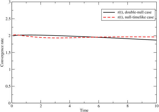
Figure 1: Convergence rate $r(t)$, in the interval $0\leq t\leq 10$, of the numerical solution $\Phi$ for the double-null case (6) and null-timelike case (7), with $b=0.1$ and $a=1$.

III.2 Stability Tests

Test runs for the two systems (6) and (7) confirmed the results for the well-posedness of the analytic problem found in wpsw :

• For $a<0$, both problems are ill posed. Numerical instability is evident and the runs quickly crash.

• For the double-null system (6) with $a=1$ and $|b|>0$, there are exponentially growing modes but the runs are numerically stable and convergent.

• For the null-timelike system (7) with $a=1$ and $|b|<a$, there are no growing modes. For $|b|>a$, there are exponentially growing modes, but the runs are numerically stable and convergent.

• In all simulations for $a>0$, the wave remains smooth and there is no sign of numerical instability.

Figure 2 displays the effect of the lower order terms for the evolution of the double-null system with $a=2b=1$, for the initial pulse (34) and source $S=0$. The fastest growing mode in the analytic problem is not evident at the early time $t=1$ but becomes dominant at $t=25$. The solution continues to grow but remains smooth, showing no sign of a numerically induced instability. There is more extreme growth for the case $a=b=1$.

For the null-timelike system (6), the quasi-normal modes

$$\Phi=e^{st+i(\omega_{1}x+\omega_{2}y)}$$ (37)

have growth (decay) rate $\Re s$ given by (16). Consequently, $\Re s<0$ for $|b|<a$ and the modes are damped. Simulations for $a=1$ and $b=0.5$ show no sign of growth and the wave decays at late times. For $b>a$, (16) implies that the dominant growing mode satisfies $\omega_{2}=-b\omega_{1}/a$ so that the wave develops a symmetry along the lines $x-(b/a)y=const$. For the neutrally stable case $a=b=1$ illustrated in Fig. 3, initial growth of the critical mode with $\omega_{2}=-\omega_{1}$ is evident at $t=5$. As shown in Fig. 4, this neutrally stable mode does not exhibit exponential growth or decay but settles into a constant amplitude traveling wave. The late time behavior shows the expected symmetry along the diagonal lines $x-y=const$. (For $b=-a$ the symmetry switches to the diagonals $x+y=const$.)

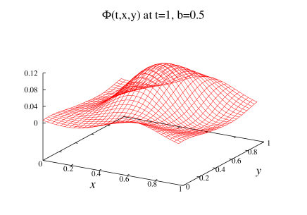
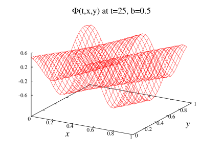
Figure 2: Snapshots of the simulation of the double-null system (6), with initial pulse (34), for $b=0.5$ and $a=1$. On the left, at $t=1$, the growing mode is barely visible. On the right, at $t=25$, the growing mode dominates but the smoothness indicates no sign of a numerically induced instability. The case $b=1$ shows more extreme growth.

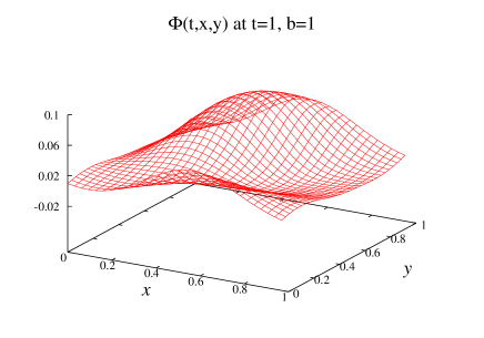
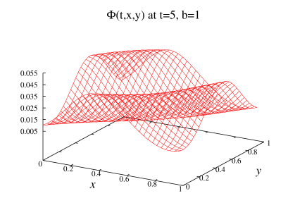
Figure 3: Snapshots of the simulation of the null-timelike system (7), with initial pulse (34) for the neutrally stable case $b=a=1$ At $t=1$ (left), the pulse has begun to develop asymmetry. At $t=5$ (right), the critical mode with symmetry along the diagonal lines has begun to form.

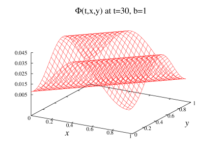
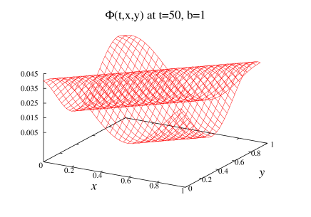
Figure 4: Late time behavior of the null-timelike system (7), with initial initial pulse (34), for the neutrally stable case $b=a=1$. The late time behavior at $t=30$ (left) and $t=50$ (right) shows that critical mode maintains a constant amplitude as the wave travels.

III.3 Simulations of the double-null problem

Here we present simulations of the double-null problem (6) for the case $a=1$ and $b=0.1$ where no growing modes are excited. First, for the compact initial pulse (34) with source $S=0$, Fig’s. 5 and 6 show that two qualitative features emerge on the order of a few crossing times: the $y$-dependence become uniform and the wave freezes in shape. This behavior can be inferred from the integral

$$\int dxdy\Phi_{t}\bigg{(}\partial_{t}(\Phi_{x}+a\Phi)-\partial_{y}^{2}\Phi+2b\partial_{y}\Phi\bigg{)}=0$$ (38)

which implies

$$\partial_{t}\int dxdy(\partial_{y}\Phi)^{2}=-2a\int dxdy{\Phi_{t}}^{2}-4b\int dxdy{\Phi_{t}}\partial_{y}\Phi.$$ (39)

Thus, for $b<<a$, the $y$-dependence monotonically becomes homogeneous as $\Phi_{t}\rightarrow 0$ and the waveform freezes as it propagates with zero coordinate velocity along the characteristic in the $t$-direction.

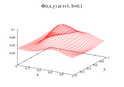
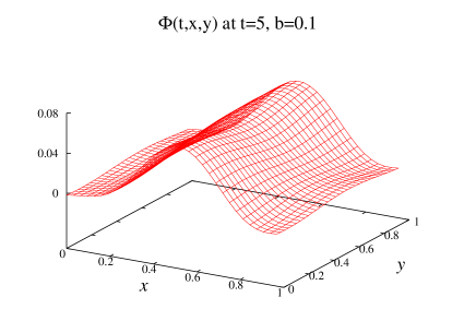
Figure 5: Early time simulation of the double-null problem for $b=0.1$ and $a=1$ with initial data (34) and source $S=0$. At $t=1$ (left plot) the wave has undergone little change but at $t=15$ (right plot) it begins to homogenize in the $y$=direction.

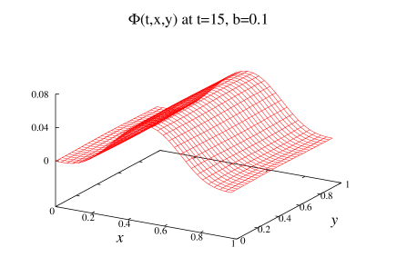
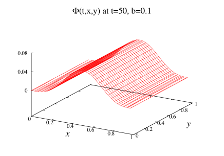
Figure 6: Late time simulation of the double-null problem for $b=0.1$ and $a=1$ with initial data (34) and source $S=0$. At $t=15$ (left plot) the wave has become uniform in the $y$-direction. At this time the wave has settled into a stable mode and its shape has frozen, as evident from comparison with the right plot at $t=50$.

Next we present simulations with vanishing initial data and a non-vanishing source. As an indication of what to expect, consider the example

$$S=\delta(x-\frac{1}{2})\partial_{t}\psi(t),$$

where $\psi(t)$ is a compact signal in time. The corresponding solution of (6) is

$$\Phi(t,x)=\frac{e^{-a/2}}{1-e^{-a}}e^{-ax}\psi(t),\quad 0\leq x<\frac{1}{2}$$

$$\Phi(t,x)=\frac{e^{a/2}}{1-e^{-a}}e^{-ax}\psi(t),\quad\frac{1}{2}<x<1.$$

Notably, a signal emitted in the forward $x$-direction instantaneously circuits the closed lightlike line and returns to the source.

Figures 7 and 8 present snapshots of the numerical evolution of the double-null problem with the compact pulse-shaped source (35) for $b=0.1$ and $a=0.5$. In Fig. 7, at $t=2.1$ just after the source has turned on, it is clear that the signal has instantaneously propagated around the closed lightlike curve in the $x$-direction. The effect of the $a$-term is to damp the signal as it returns to the source.

After the source is turned off at $t=8$, the wave continues to spread in the $y$-direction as its amplitude decays. At $t=10$, there is little evidence of the original compactness of the source. At late times, as shown in Fig. 8, the wave continues to decay as it becomes more uniform.

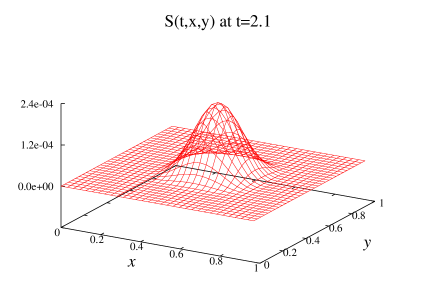
Figure 7: Simulation of the double-null problem for $b=0.1$ and $a=0.5$ with compact source (35). The left plot shows the shape of the source, at $t=2.1$, just after it has been turned on. At this same time, the right plot shows that the resulting wave has instantaneously propagated around the closed lightlike line in the $x$-direction.

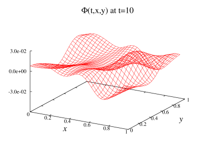
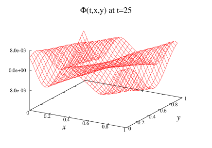
Figure 8: The propagation of the signal several crossing times after the source (35) has turned off for the double-null problem with $b=0.1$ and $a=0.5$. At $t=10$ (left plot), the wave has spread in the $y$-direction and there is no remaining evidence of the original compactness of the source. The plot at $t=25$ (right) shows that the solution continues to slowly decay as it becomes more uniform.

III.4 Simulations of the null-timelike problem

Here we present simulations of the null-timelike problem (7), for the case $a=1$ and $b=0.1$ where no growing modes are present. Now the $t$-direction is no longer characteristic and there are waves propagating in both the $\pm x$-directions. For simulations with source $S=0$, an analysis analogous to that leading to (39) for the double-null problem gives

$$\partial_{t}\int dxdy\bigg{(}(\partial_{x}\Phi)^{2}+(\partial_{y}\Phi)^{2}\bigg{)}=-2a\int dxdy{\Phi_{t}}^{2}-4b\int dxdy{\Phi_{t}}\partial_{y}\Phi.$$ (40)

For $b<<a$, (40) implies that the amplitude decays monotonically as $\Phi_{t}\rightarrow 0$. As in the double-null problem, the simulations with initial pulse (34) show that the $y$-dependence becomes uniform after a few crossing times, as illustrated in Fig. 9. However, the $x$-dependence persists as the wave decays, as can be understood in terms of the damping rate (16) for the quasi-normal modes. After the $y$-dependence has damped out, i.e. as $\omega_{2}\rightarrow 0$, (16) reduces to

$$\Re s\rightarrow-\frac{a}{1+(a^{2}/\omega_{1}^{2})}$$ (41)

so that the long wavelength $x$-dependence damps very slowly as $\Phi\rightarrow const$.

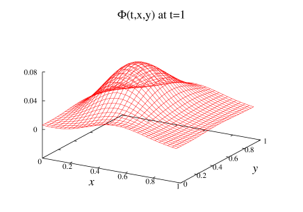
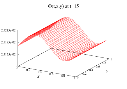
Figure 9: Evolution of the null-timelike problem for $b=0.1$ and $a=1$ with initial pulse (34) and source $S=0$. At $t=1$ (left plot) the wave has undergone little change. At $t=15$ (right plot) the wave has become uniform in the $y$-direction and has settled into a long wavelength mode traveling in the $x$-direction.

Next, we present snapshots of the simulation of the null-timelike problem for $b=0.1$ and $a=0.5$ with vanishing initial data and the compact pulse-shaped source $S$ given by (35). The left snapshot in Fig. 10 at $t=2.1$, just after the source is turned on, shows that the signal has instantaneously propagated around the closed lightlike line in the $x$-direction. The right snapshot at $t=25$ shows that at late times the wave has homogenized in the $y$-direction as it decays into a long wavelength mode of diminishing amplitude traveling in the $x$-direction.

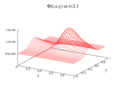
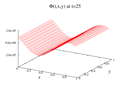
Figure 10: Simulation of the null-timelike problem for $b=0.1$ and $a=0.5$ with compact source (35). The left snapshot at $t=2.1$, just after the source is turned on, shows that the signal has instantaneously propagated around the closed lightlike line in the $x$-direction, very similar to the corresponding double-null problem illustrated in Fig. 7. The late time behavior in the right snapshot at $t=25$ shows that the wave homogenizes in the $y$-direction as it decays, but in a quite different manner than the decay in the double-null problem illustrated in Fig. 8.

IV Marching algorithm for the half-plane problem

We first consider the initial-boundary value problem for

$$\partial_{t}(\partial_{x}\Phi+a\Phi)=\partial_{x}^{2}\Phi$$ (42)

with the semi-discrete approximation

$$\partial_{t}\bigg{(}D_{0x}\Phi+a\Phi\bigg{)}=D_{+x}D_{-x}\Phi,$$ (43)

in the half-plane $0\leq x\leq\infty$, with Dirichlet boundary conditions at the inner time-like boundary $x=0$. The lines $t=\text{const}$ are outgoing characteristics. For this problem, there is no periodicity in the $x$ direction so that the discrete Fourier approach of Sec. II.1 is no longer appropriate for a numerical algorithm. Although a different spectral (or pseudo-spectral) algorithm could be adopted, we pursue a local finite difference approach. In this case the method of lines is not applicable because reduction of (43) to a first order system does not lead to a system of ordinary differential equations in time. Instead, we construct a marching algorithm along the outgoing characteristics, as first developed in march .

We discretize (43) in both time and space on a grid with boundary at $x=0$. This leads to the finite difference equation

$$D_{0t}(D_{0x}\Phi+a\Phi)=D_{+x}D_{-x}\Phi,$$ (44)

where $t_{n}=n\Delta t$. We denote $\Delta t=\lambda\Delta x=\lambda h$, in terms of the Courant factor $\lambda$. Setting $\Phi^{n}_{j}=\Phi(n\lambda h,jh)$ and centering (44) about the virtual grid point $(n+\frac{1}{2},j-\frac{1}{2})$, we use the second order accurate approximations

$$\partial_{t}D_{0}\Phi=\frac{\Phi^{n+1}_{j}-\Phi^{n+1}_{j-1}-\Phi^{n}_{j}+\Phi^{n}_{j-1}}{\lambda h^{2}},$$ (45)

$$\partial_{t}\Phi=\frac{\Phi^{n+1}_{j}+\Phi^{n+1}_{j-1}-\Phi^{n}_{j}-\Phi^{n}_{j-1}}{2\lambda h},$$ (46)

$$\partial_{x}\Phi=\frac{\Phi^{n+1}_{j}-\Phi^{n+1}_{j-1}+\Phi^{n}_{j}-\Phi^{n}_{j-1}}{2h},$$ (47)

and

$$D_{+}D_{-}\Phi=\frac{\Phi^{n+1}_{j}-2\Phi^{n+1}_{j-1}+\Phi^{n+1}_{j-2}+\Phi^{n}_{j+1}-2\Phi^{n}_{j}+\Phi^{n}_{j-1}}{2h^{2}}.$$ (48)

With these approximations (44) is equivalent to

$$\frac{\Phi^{n+1}_{j}-\Phi^{n+1}_{j-1}-\Phi^{n}_{j}+\Phi^{n}_{j-1}}{\lambda h^{2}}+\frac{a(\Phi^{n+1}_{j}+\Phi^{n+1}_{j-1}-\Phi^{n}_{j}-\Phi^{n}_{j-1})}{2\lambda h}=\frac{\Phi^{n+1}_{j}-2\Phi^{n+1}_{j-1}+\Phi^{n+1}_{j-2}+\Phi^{n}_{j+1}-2\Phi^{n}_{j}+\Phi^{n}_{j-1}}{2h^{2}}$$ (49)

so that

$$\bigg{(}1+(ah/2)-(\lambda/2)\bigg{)}\Phi^{n+1}_{j} = \bigg{(}1-(ah/2)-\lambda\bigg{)}\Phi^{n+1}_{j-1}+(\lambda/2)\Phi^{n+1}_{j-2}+(\lambda/2)\Phi^{n}_{j+1}$$ (50)

$$+ \bigg{(}1+(ah/2)-\lambda\bigg{)}\Phi^{n}_{j}+\bigg{(}-1+(ah/2)+(\lambda/2)\bigg{)}\Phi^{n}_{j-1},$$

which determines $\Phi^{n+1}_{j}$, in terms of $(\Phi^{n+1}_{j-1},\Phi^{n+1}_{j-2},\Phi^{n}_{j+1},\Phi^{n}_{j},\Phi^{n}_{j-1})$. For $a=0$, this is identical to the approximation obtained in march which was obtained from an integral identity satisfied by a scalar wave at the corners of a characteristic parallelogram.

The marching algorithm based upon (50) proceeds as follows. Let $\Phi^{n}_{j}$ be given on time level $t_{n}$ and let $\Phi^{n+1}_{0}$ and $\Phi^{n+1}_{1}$ be given on time level $t_{n+1}$. Then (50) determines $\Phi^{n+1}_{2}$ and then, sequentially, $\Phi^{n+1}_{3},\Phi^{n+1}_{4},\Phi^{n+1}_{5}\dots$. After updating the $t_{n+1}$ time level, this outward march along the characteristic is repeated to update $t_{n+2}$. The required initial data are $\Phi^{0}_{j}$, which are supplied by the characteristic initial data $\Phi(0,x)$. The required boundary data are $\Phi^{n}_{0}$, which are supplied by the Dirichlet boundary data $\Phi(t,0)$. In addition, a start-up algorithm is needed to obtain $\Phi^{n}_{1}$ (see below).

The stability of the algorithm can be determined by analyzing the behavior of the Fourier-Laplace modes

$$\Phi^{n}_{j}=e^{st_{n}}e^{i\omega jh},\quad t_{n}=n\lambda h.$$ (51)

Substitution into (49) leads, after some algebra, to the amplification factor

$$\hat{Q}=e^{s\lambda h}=\frac{1-\lambda\sin^{2}(\omega h/2)+i\cot(\omega h/2)(\lambda\sin^{2}(\omega h/2)-(ah/2))}{1-\lambda\sin^{2}(\omega h/2)-i\cot(\omega h/2)(\lambda\sin^{2}(\omega h/2)+(ah/2))}.$$ (52)

Thus, as found in march , $|\hat{Q}|=1$ for the case $a=0$, i.e. the algorithm is unimodular. For $a>0$, $|\hat{Q}|<1$ and the algorithm is damped. The algorithm is unstable for $a<0$.

An algorithm is unconditionally stable if $|\hat{Q}|\leq 1$ and stable if $|\hat{Q}|$ has an upper bound independent of the values of $\omega$ and $h$. The above algorithm is unconditionally stable for $a\geq 0$. In addition, it is convergent provided $\lambda<1$ so that the Courant-Friedrichs-Lewy (CFL) condition (that the numerical domain of dependence contain the analytic domain of dependence) is satisfied. However, the unimodular stability for the limiting case $a=0$ makes the algorithm prone to instabilities when extended to higher dimensional systems. In addition, see luisdiss for a discussion of potential nonlinear instabilities and a technique to control them by introducing artificial dissipation into (49). Modulo such higher order terms, the basic finite difference approximation (49) appears to be the unique 2-level algorithm which is stable, convergent and second order accurate, i.e. we have not been able to find any other other algorithm with these properties.

The generalization of the marching algorithm to higher dimensions is straightforward using the techniques described in march . However, instabilities can arise from the introduction of additional lower order terms. A critical case is the 2-spatial dimension wave equation

$$\partial_{t}(\partial_{x}\Phi+a\Phi)=\partial_{x}^{2}\Phi+\partial_{y}^{2}\Phi-2b\partial_{y}\Phi,\quad a>0.$$ (53)

The corresponding CFL condition is $\lambda<1/2$, which is determined by the characteristics in the $(t,\pm y)$ planes. As before, we discretize the $y$-dependence on a periodic grid and write $\Phi^{n}_{j_{1},j_{2}}=\Phi(t_{n},x_{j_{1}},y_{j_{2}})$. We introduce the second order approximation

$$[\partial_{y}^{2}\Phi-2b\partial_{y}\Phi]^{n+1/2}_{j_{1}-1/2,j_{2}}=\frac{1}{2}(D_{+y}D_{-y}-2bD_{0y})(\Phi^{n+1}_{j_{1}-1,j_{2}}+\Phi^{n}_{j_{1}.j_{2}}),$$ (54)

which does not involve the values $\Phi^{n+1}_{j_{1},j_{2}}$ so that the marching algorithm can be extended to 2-dimension. In order to analyze the stability of the resulting marching algorithm, we consider the modes

$$\Phi^{n}_{j_{1},j_{2}}=e^{sn\lambda h}e^{i\omega_{1}j_{1}h}e^{i\omega_{2}j_{2}h}.$$ (55)

From a calculation analogous to that leading to (52), we find

$$|\hat{Q}|^{2}=\frac{\bigg{(}1-A-hB\cot(h\omega_{1}/2)\bigg{)}^{2}+\bigg{(}(A-(ah/2))\cot(\omega_{1}h/2)-hB\bigg{)}^{2}}{\bigg{(}1-A+hB\cot(\omega_{1}h/2)\bigg{)}^{2}+\bigg{(}(A+(ah/2))\cot(\omega_{1}h/2)+hB\bigg{)}^{2}},$$ (56)

where

$$A=\lambda(\sin^{2}(h\omega_{1}/2)+\sin^{2}(h\omega_{2}/2))$$ (57)

and

$$B=\frac{\lambda b\sin(\omega_{2}h)}{2}.$$ (58)

Thus

$$|\hat{Q}|^{2}=1+\frac{-4hB\cot(h\omega_{1}/2)-2ahA\cot^{2}(h\omega_{1}/2)}{\bigg{(}1-A+hB\cot(h\omega_{1}/2)\bigg{)}^{2}+\bigg{(}(A+(ah/2))\cot(h\omega_{1}/2)+hB\bigg{)}^{2}}.$$ (59)

For $b=0$ and $a\geq 0$, $|\hat{Q}|\leq 1$ and the algorithm is unconditionally stable.

In order to analyze the effect of $b\neq 0$, first consider the continuum approximation $h\approx 0$ with bounded values of $(\omega_{1},\omega_{2})$, for which

$$\bigg{(}-4hB\cot(h\omega_{1}/2)-2ahA\cot^{2}(h\omega_{1}/2)\bigg{)}\sin^{2}(h\omega_{1}/2)\approx-\frac{\lambda h^{3}}{2}\bigg{(}2b\omega_{1}\omega_{2}+a(\omega_{1}^{2}+\omega_{2}^{2})\bigg{)}\leq\frac{\lambda h^{3}}{2}(|b|-a)(\omega_{1}^{2}+\omega_{2}^{2}),$$ (60)

so that, referring to (56), $|\hat{Q}|\leq 1$ for $|b|\leq a$ and the algorithm remains unconditionally stable. More generally in this approximation,

$$|\hat{Q}|^{2} \approx 1-\frac{2\lambda h\bigg{(}2b\omega_{1}\omega_{2}+a(\omega_{1}^{2}+\omega_{2}^{2})\bigg{)}}{\omega_{1}^{2}+a^{2}}$$

$$\leq 1-\frac{2\lambda h\bigg{(}a(\omega_{2}+{b\over a}\omega_{1})^{2}-{b^{2}\over a}\omega_{1}^{2}\bigg{)}}{\omega_{1}^{2}+a}\leq 1+\frac{2\lambda hb^{2}}{a},$$

so that the growth rate is bounded independent of $(\omega_{1},\omega_{2})$. Hence the algorithm remains numerically stable but reflects the existence of exponentially growing modes in the analytic problem. In this approximation, note that for $a=0$ and $b\neq 0$ that

$$|\hat{Q}|^{2}\approx 1-4\lambda b{\omega_{2}\over\omega_{1}},$$ (61)

so there would be a catastrophic instability for $(-b\omega_{2})/\omega_{1}\rightarrow\infty$. This again reflects the important role of the condition $a>0$ in determining the well-posedness of the problem.

Next, for $a>0$, consider the limiting cases where either $\omega_{1}\rightarrow\infty$ or $\omega_{2}\rightarrow\infty$, or both, as $h\rightarrow 0$. We express (59) in the form

$$|\hat{Q}|^{2}=1+\frac{-2h\bigg{(}B(Aa)^{-1/2}+(Aa)^{1/2}\cot(h\omega_{1}/2)\bigg{)}^{2}+2hB^{2}(Aa)^{-1}}{\bigg{(}1-A+hB\cot(h\omega_{1}/2)\bigg{)}^{2}+\bigg{(}(A+(ah/2))\cot(h\omega_{1}/2)+hB\bigg{)}^{2}},$$ (62)

so that

$$|\hat{Q}|^{2} \leq 1+\frac{2hB^{2}(Aa)^{-1}}{\bigg{(}1-A+hB\cot(h\omega_{1}/2)\bigg{)}^{2}+\bigg{(}(A+(ah/2))\cot(h\omega_{1}/2)+hB\bigg{)}^{2}}$$ (63)

$$\leq 1+\frac{2hb^{2}/a}{\bigg{(}1-A+hB\cot(h\omega_{1}/2)\bigg{)}^{2}+\bigg{(}(A+(ah/2))\cot(h\omega_{1}/2)+hB\bigg{)}^{2}},$$

where we have used the identity $\sin^{4}\theta=4\sin^{2}(\theta/2)\cos^{2}(\theta/2)$ to obtain

$$B^{2}A^{-1}=\frac{b^{2}\sin^{2}(h\omega_{2}/2)\cos^{2}(h\omega_{2}/2)}{\sin^{2}(h\omega_{1}/2)+\sin^{2}(h\omega_{2}/2)}\leq b^{2}.$$ (64)

We observe that uncontrolled growth can only occur if there are values of $(\omega_{1},\omega_{2})$ such that the denominator in (63) vanishes, which requires

$$hB=-\frac{1-A}{\cot(h\omega_{1}/2)}=-(A+\frac{ah}{2})\cot(h\omega_{1}/2).$$ (65)

The second equality in (65) implies

$$\cot^{2}(h\omega_{1}/2)=\frac{1-A}{A+(ah/2)}=\frac{1-\lambda\bigg{(}\sin^{2}(h\omega_{1}/2)+\sin^{2}(h\omega_{2}/2)\bigg{)}}{\lambda\bigg{(}\sin^{2}(h\omega_{1}/2)+\sin^{2}(h\omega_{2}/2)\bigg{)}+(ah/2)},$$ (66)

so that solving for $\sin^{2}(h\omega_{1}/2)$ gives

$$\sin^{2}(h\omega_{1}/2)=\frac{\lambda\sin^{2}(h\omega_{2}/2)+(ah/2)}{1-\lambda+(ah/2)}$$ (67)

as a necessary condition for an unstable mode. However, because $B=O(h)$, a straightforward analysis shows that the first equality in (65) rules out such modes for reasonably small values of $h$. As an example, consider the mode $\sin^{2}(h\omega_{1}/2)=\sin^{2}(h\omega_{2}/2)=1/2$, (67) with $\lambda=(1/2)-(ah/4)$, which satisfies (67) and is consistent with the Courant condition $\lambda<1/2$. Then the first equality in (65) would require,

$$|b|h=2|1-\lambda^{-1}|,$$ (68)

which would not be satisfied. The robust stability boundary test described in Sec. V.1 verifies this conclusion that the marching algorithm is stable.

In Sec. V, we present tests and simulations of the null-timelike problem

$$\partial_{t}(\partial_{x}\Phi+a\Phi)=\partial_{x}\bigg{(}(1-x)^{2}\partial_{x}\Phi\bigg{)}+\partial_{y}^{2}\Phi-2b\partial_{y}\Phi,\quad 0\leq x\leq 1,\quad 0\leq y<1,\quad t\geq 0,$$ (69)

with periodicity in $y$. We assign Dirichlet boundary values at $x=0$. The boundary at $x=1$ is an ingoing characteristic surface and requires no boundary condition. It is analogous to the boundary at null infinity obtained by conformal compactification. The finite difference approximation (48) is modified according to

$$\partial_{x}\bigg{(}(1-x)^{2}\partial_{x}\Phi\bigg{)}=(1-x)^{2}\partial^{2}_{x}\Phi-2(1-x)\partial_{x}\Phi\approx(1-x)^{2}D_{+x}D_{-x}\Phi-2(1-x)D_{0x}\Phi,$$ (70)

which is evaluated at the mid-point $(j_{1}-1/2,j_{2})$ at time $t_{n+1/2}$ by

$$(1-x)^{2}D_{+x}D_{-x}\Phi=\frac{1}{2}(1-x_{j_{1}-1})^{2}D_{+x}D_{-x}\Phi^{n+1}_{j_{1}-1,j_{2}}+\frac{1}{2}(1-x_{j_{1}})^{2}D_{+x}D_{-x}\Phi^{n}_{j_{1},j_{2}}$$ (71)

and

$$-2(1-x)D_{0x}\Phi=-(1-x_{j_{1}-1/2})D_{0x}\bigg{(}\Phi^{n+1}_{j_{1}-1/2,j_{2}}+\Phi^{n}_{j_{1}-1/2,j_{2}}\bigg{)}.$$ (72)

These approximations, along with the previous second order approximations for the other terms in the wave equation, allow the values of $\Phi^{n+1}_{N_{1},j_{2}}$ at the outer (characteristic) boundary $x=1$ to be updated in terms of values previously determined by the marching algorithm. The startup algorithm at the inner boundary $x=0$ is more complicated since an approximation for $\partial_{x}^{2}\Phi$ requires a minimum of three grid points. In order to circumvent this difficulty we write

$$\partial_{x}^{2}\Phi=\lambda\partial_{x}\partial_{t}\Phi-\partial_{x}(\lambda\partial_{t}-\partial_{x})\Phi.$$ (73)

Here the first term on the right hand side only requires a two-point stencil as in (45). In addition, the second term can be approximated to second order by a stencil involving only the first two points on the upper time level,

$$\partial_{x}(\lambda\partial_{t}-\partial_{x})\Phi^{n+1/2}_{1/2,j_{2}}=\frac{1}{h}D_{0x}(\Phi^{n+1}_{1/2,j_{2}}-\Phi^{n}_{3/2,j_{2}})=\frac{1}{h^{2}}(\Phi^{n+1}_{1,j_{2}}-\Phi^{n+1}_{0,j_{2}}-\Phi^{n}_{2,j_{2}}+\Phi^{n}_{1,j_{2}}).$$ (74)

Along with the other terms in the wave equation, this can be used to determine $\Phi^{n+1}_{1,j_{2}}$ in terms of the Dirichlet boundary data $\Phi^{n+1}_{0,j_{2}}$ and previously determined values.

V Simulation of the null-timelike strip problem

Here we apply the marching algorithm described in Sec. IV to simulate the initial-boundary value problem for the wave equation (69),

$$\partial_{t}(\partial_{x}\Phi+a\Phi)=\partial_{x}\bigg{(}(1-x)^{2}\partial_{x}\Phi\bigg{)}+\partial_{y}^{2}\Phi-2b\partial_{y}\Phi,\quad t\geq 0,$$ (75)

in the strip $0\leq x\leq 1$, $0\leq y<1$, with periodicity in the $y$-direction. We assign initial data and Dirichlet boundary data

$$\Phi(0,x,y)=f(x,y)\quad\Phi(t,0,y)=q(t,y).$$ (76)

The principle part of the wave operator in (75) corresponds to the metric

$$ds^{2}=-4(1-x)^{2}dt^{2}-4dtdx+dy^{2}.$$

This implies that the boundary at $x=1$ is an ingoing characteristic hypersurface so that no boundary condition should be applied there.

This strip problem with $a>0$ was shown to be well posed in wpsw , where an energy estimate established that the solution and its derivatives remain bounded. We demonstrate this by the stability and convergence tests in Sec’s. V.1 and V.2. The simulations in Sec’s V.3 illustrate the effects of the lower order $a$-term.

V.1 Stability

The analysis in Sec. IV showed that the marching algorithm for the problem (75) is stable for $a>0$. For $a<0$, the problem is ill posed and numerical stability cannot be expected. We confirm these results by carrying out robust stability boundary tests robust based upon random initial and boundary data. The test is implemented using a random number generator that changes at each time-step. The test was run on a grid of size $N\times N=64^{2}$, with $h=\Delta x=1/N$ and timestep $\Delta t=h/5$, with an amplitude for the random noise of $A=1$, for a time $t=10$. The graph of the time dependence of the $L_{\infty}$ norm for the case $a=b=1$ is shown in Figure 11. There is no sign of numerical instability.

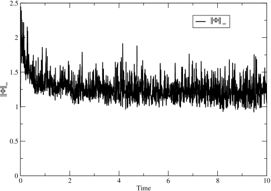
Figure 11: Time dependence of the $L_{\infty}$ norm $||\Phi||_{\infty}$ for the robust stability boundary test with $a=b=1$.

The instability for cases $a<0$ is not as pronounced as for the tests of the Cauchy problem. This is because the unstable modes are propagated off the grid through the characteristic boundary at $x=1$. Consequently, the robust stability test is not as effective as in the case of the strip problem between two timelike boundaries. Nevertheless, rapid unstable growth is evident for sufficiently negative values of $a$.

V.2 Convergence

We carry out two convergence tests. In the first, the initial-boundary data is based upon the exact solution for $b=0$,

$$\Phi=e^{st}\phi(x)\cos(\omega y),\quad s=-\frac{\omega^{2}}{a}$$ (77)

where

$$\phi(x)=e^{sx/(1-x)}.$$ (78)

In this test we set $\omega=2\pi$ and $a=10$ so that the exponential decay of the solution can be resolved with reasonable sized grids $N_{A}\times N_{A}$, with $N_{A}=64/A$ in the ratio $A=(1,2)$. On these grids, the convergence to the exact solution is measured with Courant factor $\Delta t_{A}/h_{A}=1/5$ in the interval $0\leq t\leq 1$. The convergence rate $r(t)\approx 2$, shown in the left plot of Fig. 12, is in excellent accord with the second order finite difference approximations.

We also test Cauchy convergence for the case $a=b=1$ for the simulation of the initial pulse

$$\Phi(0,x,y) = A\left[(x-x_{1})(y-y_{1})(x-x_{2})(y-y_{2})\right]^{4},\quad x_{1}\leq x\leq x_{2},\,y_{1}\leq y\leq y_{2},$$

$$\Phi(0,x,y) = 0,\quad{\rm otherwise},$$ (79)

with vanishing boundary data. We take $x_{1}=y_{1}=0.1$, $x_{2}=y_{2}=0.9$ and amplitude $A=10^{5}$. The Cauchy convergence rate $r(t)$, measured for three grids of size $N_{A}\times N_{A}$, with $N_{A}=128/A$, with $A=(1,2,4)$,and Courant factor $\Delta t_{A}/h_{A}=1/5$, is shown in the right plot of Fig. 12. We again obtain clean second order convergence $r(t)\approx 2$.

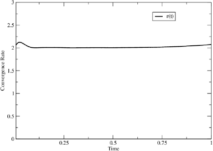
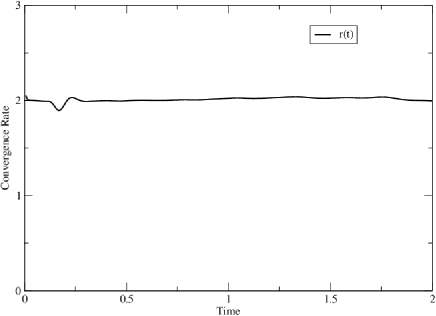
Figure 12: Left: Convergence rate $r(t)$ to the exact solution (77) in the interval $0\leq t\leq 1$, with $a=10$ and $b=0$.
Right: Cauchy convergence rate $r(t)$ for simulation of the initial pulse (79) with $a=b=1$.

V.3 Damping, radiation tails and the $a$-term

In order to reveal the effects of the $a$-term in (75) first consider the exact 1-dimensional solutions for the case $a=0$,

$$\Phi(t,x)=F_{1}(t)+F_{2}(t+\frac{1}{1-x}).$$ (80)

Here $F_{1}(t)$, with $F_{2}=0$, describes a purely outgoing wave emanating from the inner boundary. For the simulation of such a purely outgoing wave, we choose the pulsed signal

$$F_{1}(t)=A[(t-t_{1})(t-t_{2})]^{4},\quad t_{1}=0.2,\,t_{2}=0.8,\quad F_{1}(t)=0\,\text{for}\,t<t_{1}\,\text{and}\,t>t_{2},$$

corresponding to the initial and boundary data

$$\Phi(0,x)=0\,,\quad\Phi(t,0)=F_{1}(t).$$ (81)

We choose the amplitude $A=10^{4}$ to make the peak of order unity. For $a=0$ the profile $\Phi(t,1)$ of the waveform passing through the outer boundary is identical with the inner boundary data, i.e. $\Phi(t,1)=F_{1}(t)$, and the error is the order of machine precision. For $a>0$. the solution to (75) resulting from the data (81) is no longer given by (80) and shows the effects of backscatter. Figure 13, which compares the waveforms $\Phi(t,1)$ resulting from the initial data (81) for the cases $a=0$, $a=0.1$ and $a=1$, illustrates the damping of the outgoing waveform due to the $a$-term. The $a$-term produces a tail to the waveform which decays on a time scale increasing with the size of $a$.

Snapshots of $\Phi(t,x)$ for $a=1$ are given in Fig. 14 at times $t=0.5$ (in the middle of the signal $F_{1}(t)$) and $t=2.0$ (after the signal has turned off). The snapshots exhibit a distinctive, almost horizontal slope near the outer boundary, which can be explained by evaluating (75) at $x=1$,

$$\partial_{t}\bigg{(}\partial_{x}\Phi(t,1)-a\Phi(t,1)\bigg{)}=0,\,\quad a=1,$$ (82)

which implies

$$\partial_{x}\Phi(t,1)=-\Phi(t,1),$$ (83)

since $\Phi(0,x)=0$. During the signal, when $\Phi(t,1)$ is large and positive, this results in a negative slope at $x=1$ but during the tail, as $\Phi(t,1)$ decays to zero, this slope becomes very small.

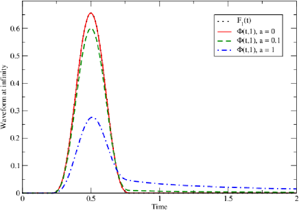
Figure 13: The waveform at the outer characteristic boundary corresponding to the purely outgoing data (81). The $a$-term produces a tail which decays on a time scale increasing with $a$.

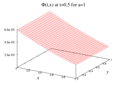
Figure 14: Snapshots $\Phi(t,x)$ for $a=1$, with boundary data (81). The left plot in the middle of the signal at $t=0.5$ is dominated by the negative slope at the outer boundary resulting from (83). The right plot at $t=2$ shows that this slope becomes small during the tail decay.

These 1-dimensional results shed light on the behavior in the 2-dimensional case obtained by adding a compact $y$-dependence to the pulsed boundary data,

$$\Phi(0,x,y)=0\,,\quad\Phi(t,0,y)=A[(t-t_{1})(t-t_{2})(y-y_{1})(y-y_{2})]^{4},\quad(t_{1},y_{1})=0.2,\,(t_{2},y_{2})=0.8.$$ (84)

The left plot of Fig. 15 shows a snapshot of the wave in the middle of the signal at $t=0.5$. Where the $y$-dependence of the pulse is peaked, it is similar to the left plot Fig. 14 for the 1-dimensional case. Similarly the snapshot during the tail decay at $t=2$ in the right plot of Fig. 15 is almost identical to the right plot of Fig. 14, differing only by some backscatter of the original pulse.

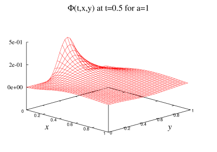
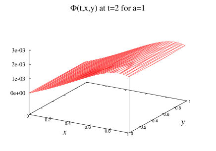
Figure 15: Snapshots $\Phi(t,x,y)$ for $a=1$ and $b=0$, with pulse shaped boundary data (84) during the middle of the signal at $t=0.5$ (left plot) and during the tail decay at $t=2$ (right plot). The similarity to the 1-dimensional case in Fig. 14 is evident.

VI Summary

Analytic results regarding the importance of the $a$-term for the well-posedness of the characteristic initial-boundary value problems for the wave equation have been extended to the finite difference formulation. Based upon these results, we have developed computational evolution algorithms for the scalar wave equation in characteristic coordinates. We proved the numerical stability of the algorithms analytically, by means of both Fourier-Laplace theory and the energy method. The approach allowed us to individually test the finite difference code for the pure Cauchy problem and for the initial-boundary value problem in a strip. The main result for both problems is that numerical stability is controlled by the condition $a>0$, an important feature which had been overlooked in treatments of the characteristic initial value problem for the wave equation.

The pure Cauchy problem was implemented with periodic boundary conditions so that characteristics formed closed timelike curves. This gave rise to simulations in which a signal propagated instantaneously back to the source. The evolution code for the strip problem, with timelike inner boundary and characteristic outer boundary, was modeled upon the characteristic marching algorithm, which has been used for characteristic evolution in general relativity. The knowledge gained from the model problems considered here should be of benefit to a better understanding of the gravitational case and other applications of characteristic evolution lr .

- (1) H.-O. Kreiss and J. Winicour, “The well-posedness of the null-timelike boundary problem for quasilinear waves”, Class. Quantum Grav. 28,145020 (2011).
- (2) H-O. Kreiss and J. Lorenz, “Initial-Boundary Value Problems and the Navier-Stokes Equations”, (Academic Press, New York, 1989), Reprint Siam Classics (2004).
- (3) M. van der Burg, H. Bondi and A. Metzner, “Gravitational waves in general relativity VII. Waves from axi-symmetric isolated systems”, Proc. R. Soc. London A, 269, 21 (1962).
- (4) R. Sachs. “Gravitational waves in general relativity VIII. Waves in asymptotically flat space-time”, Proc. R. Soc. London A, 270, 103 (1962).
- (5) R. Penrose, Phys. Rev. Letters, 10 66 (1963).
- (6) L. Tamburino and J. Winicour, “Gravitational fields in finite and conformal Bondi frames”, Phys. Rev., 150, 1039 (1966).
- (7) J, Winicour, “Characteristic evolution and matching”, Living Rev. Relativity 12 3 (2009).
- (8) B. Gustafsson, H-O Kreiss and J. Oliger, “Time Dependent Problems and Difference Methods”, John Wiley and Sons, Inc (1995)
- (9) EinsteinToolkit home page: http://www.einsteintoolkit.org.
- (10) Cactus Computational Toolkit home page: http://www.cactuscode.org
- (11) R. Gómez, J. Winicour, and R. Isaacson, “Evolution of scalar fields from characteristic data”, J. Comp. Phys. 98, 11 (1992).
- (12) L. Lehner, “A dissipative algorithm for wave-like equations in the characteristic formulation”, J. Comp. Phys. 149, 59 (1999).
- (13) “Boundary conditions in linearized harmonic gravity”, B. Szilágyi, B. Schmidt and J. Winicour, Phys. Rev. D 65, 064015 (2002).