Average Consensus on Arbitrary Strongly Connected Digraphs with Time-Varying Topologies

Abstract

We have recently proposed a “surplus-based” algorithm which solves the multi-agent average consensus problem on general strongly connected and static digraphs. The essence of that algorithm is to employ an additional variable to keep track of the state changes of each agent, thereby achieving averaging even though the state sum is not preserved. In this note, we extend this approach to the more interesting and challenging case of time-varying topologies: An extended surplus-based averaging algorithm is designed, under which a necessary and sufficient graphical condition is derived that guarantees state averaging. The derived condition requires only that the digraphs be arbitrary strongly connected in a joint sense, and does not impose “balanced” or “symmetric” properties on the network topology, which is therefore more general than those previously reported in the literature.

I Introduction

The average consensus problem of multi-agent systems has attracted much attention in the literature (e.g., [1, 2, 3]). The problem can be described as follows. Consider a network of $n$ agents whose state is $x(k)=[x_{1}(k)\ \cdots\ x_{n}(k)]^{T}\in\mathbb{R}^{n}$ at discrete time $k=0,1,2,\ldots$. Every agent $i\in[1,n]$ interacts locally with its neighbors for the exchange of state information, and based on the obtained neighbors’ states it updates its own $x_{i}(k)$ to a new value $x_{i}(k+1)$ according to a prescribed algorithm. One aims at designing distributed algorithms by which agents may iteratively update their states such that $x(k)=x_{a}\textbf{1}$ asymptotically, where $x_{a}:=\textbf{1}^{T}x(0)/n$ is the average of the initial states and $\textbf{1}:=[1\ \cdots\ 1]^{T}\in\mathbb{R}^{n}$.

In [4] we proposed a novel algorithm which provably achieves average consensus on general strongly connected, static networks. This result extends [2, 3] in that it does not require the “balanced” property on the network topology which can be restrictive as every agent needs to maintain exactly equal amounts for incoming and outgoing information. This is realized by augmenting for each agent an additional variable $s_{i}\in\mathbb{R}$, which we call “surplus”. Each surplus $s_{i}(k)$ at time $k$ keeps track of the state change $x_{i}(k)-x_{i}(k-1)$ of agent $i$, in such a way that $\textbf{1}^{T}(x(k)+s(k))$ is time-invariant (here $s(k)=[s_{1}(k)\ \cdots\ s_{n}(k)]^{T}$) despite that the state sum $\textbf{1}^{T}x(k)$ is in general not. The idea was originated in [5] for dealing with a quantized averaging problem.

A more interesting, yet more challenging, scenario is where the agents’ network topology is dynamic, as opposed to static. In real networks, many practical factors could result in a dynamic topology. There can be unpredictable communication issues like random packet loss, link failure, and node malfunction. There might also exist deterministic, supervisory switchings among different modes of the network. A gossip-type randomized dynamic topology has been considered in [4], where we proved that an arbitrary strongly connected topology in expectation is necessary and sufficient for our surplus-based algorithm to achieve average consensus in mean-square and almost surely. In this note, we focus on dynamic network topology varying in some deterministic fashion, and design an extended surplus-based algorithm to achieve state averaging in a uniform sense (defined below). Parts of the results here are contained in the conference precursor [6].

Our main contribution is that the required connectivity condition on time-varying network topology is weakened, as compared to those previously reported in the literature. In [2], it was shown that a sufficient connectivity condition for average consensus is that the network topology at every time (possibly different) should be both strongly connected and balanced. By contrast, supported by surplus variables, we justify that average consensus can be uniformly achieved if and only if the dynamic network is jointly strongly connected (the precise definition is given in Section II). Thus for one, the “balanced” requirement at every instant is dropped; for the other, “strongly connected” is needed only in a joint sense. As to the convergence proof, we use a Lyapunov-type argument, in the spirit of [7]. Extending the algorithm in [4], we introduce a new switching mechanism, which gives rise to a suitable Lyapunov function for state evolution. Finally, when the derived result is specialized to the static network case, we effectively relax a conservative requirement on a parameter of the algorithm in [4].

There are well-known results (existence of a spanning tree jointly, e.g., [7, 8]) for achieving a general consensus over dynamic networks, as well as new conditions of cut-balanced in [9]. To further achieve the special average consensus on the initial state, either the state sum is kept invariant or there is a way of tracking the changes of the state sum. We consider arbitrary strongly connected dynamic topologies where the state sum is time-varying in general, and propose additional surplus update dynamics to keep track of the state changes of individual agents. The surplus values are used in turn to influence the state update dynamics, thereby forcing the states to converge to, and only to, the initial average value.

We note that [10, 11] also addressed average consensus on general dynamic networks by employing auxiliary variables. In [10], an auxiliary variable is associated to each agent and a linear “broadcast gossip” algorithm is proposed; however, the convergence of that algorithm is not proved. Reference [11] also uses extra variables, and a nonlinear (division involved) algorithm is designed and proved to achieve state averaging on non-balanced digraphs. The idea is based on computing the stationary distribution for the Markov chain characterized by the agent network, and is thus different from consensus-type algorithms [1, 2, 3]. Moreover, the dynamic networks considered are of randomized type; consequently the algorithms and results are not directly applicable to the deterministic time-varying case studied in this note. In addition, [12] presents distributed algorithms which iteratively update a column-stochastic matrix into a doubly-stochastic one, and then embeds this matrix update into a standard consensus state update to achieve average consensus. Since the time-varying update matrices used are all column-stochastic, the state sum is invariant in [12]; this is different from the case of time-varying state sum we study here. Finally, centralized and distributed algorithms are designed in [13] to make a general static topology balanced. The algorithm may in principle be used also for dynamic networks, which would require a complete execution at each time for different topologies. This requirement might be strong for applications where networks vary fast.

The rest of the paper is organized as follows. First, in Section II we formulate the average consensus problem for deterministic time-varying networks. Then an extended surplus-based algorithm is designed in Section III, and the corresponding convergence result presented and proved in Section IV. A numerical example is shown in Section V, and finally in Section VI we state our conclusions.

II Average Consensus Problem

First, a review of graph notions relevant to this note is provided; and then, the average consensus problem on deterministic time-varying networks is formulated.

For a network of $n$ agents, we model their time-varying interconnection structure at time $k$ by a dynamic digraph $\mathcal{G}(k)=(\mathcal{V},\mathcal{E}(k))$: Each node in $\mathcal{V}=\{1,...,n\}$ stands for an agent, and each directed edge $(j,i)$ in $\mathcal{E}(k)\subseteq\mathcal{V}\times\mathcal{V}$ represents that agent $j$ communicates to agent $i$ at time $k$. For each node $i\in\mathcal{V}$, let $\mathcal{N}_{i}^{+}(k):=\{j\in\mathcal{V}:(j,i)\in\mathcal{E}(k)\}$ denote the set of its “in-neighbors”, and $\mathcal{N}_{i}^{-}(k):=\{j\in\mathcal{V}:(i,j)\in\mathcal{E}(k)\}$ the set of its “out-neighbors”. Also we adopt the convention $(i,i)\notin\mathcal{E}(k)$ and $i\notin\mathcal{N}_{i}^{+}(k),\mathcal{N}_{i}^{-}(k)$.

For the dynamic digraph $\mathcal{G}(k)$, we introduce a notion of joint connectivity over some finite time interval. In $\mathcal{G}(k)$ a node $i$ is reachable from a node $j$ if there exists a sequence of directed edges from $j$ to $i$ which respects the direction of the edges. We say $\mathcal{G}(k)$ is strongly connected if every node is reachable from every other node. For a time interval $[k_{1},k_{2}]$ define the union digraph $\mathcal{G}([k_{1},k_{2}]):=\left(\mathcal{V},\bigcup_{k\in[k_{1},k_{2}]}\mathcal{E}(k)\right)$; namely, the edge set of $\mathcal{G}([k_{1},k_{2}])$ is the union of those over the interval $[k_{1},k_{2}]$. A dynamic digraph $\mathcal{G}(k)$ is jointly strongly connected if there is $k_{1}$ such that for every $k_{0}$ the union digraph $\mathcal{G}([k_{0},k_{0}+k_{1}])$ is strongly connected.

The “joint” type connectivity notions have appeared in many previous works, e.g., [7, 14, 8]. In particular, to achieve a general consensus (where the consensus value need not be the initial average $x_{a}$), the following joint connectivity is essential. A node $v\in\mathcal{V}$ is called a globally reachable node if every other node is reachable from $v$. A dynamic digraph $\mathcal{G}(k)$ jointly contains a globally reachable node (or a spanning tree) if there is $k_{1}$ such that for every $k_{0}$ the union digraph $\mathcal{G}([k_{0},k_{0}+k_{1}])$ contains a globally reachable node. It is shown in [7, 14, 8] that a general consensus can be uniformly achieved on a dynamic digraph $\mathcal{G}(k)$ if and only if $\mathcal{G}(k)$ jointly contains a globally reachable node. This joint connectivity notion is weaker than the above “jointly strongly connected” notion, because a strongly connected union digraph $\mathcal{G}([k_{0},k_{0}+k_{1}])$ is equivalent to that every node of $\mathcal{G}([k_{0},k_{0}+k_{1}])$ is globally reachable. This notion is, however, too weak to achieve average consensus, as we will see in the necessity proof of our main result; there we show that the “jointly strongly connected” notion is, indeed, a necessary and sufficient condition for uniformly achieving average consensus.

We present several additional graph notions, which will be needed in the necessity proof of our main result. For $\mathcal{G}(k)=(\mathcal{V},\mathcal{E}(k))$ and a nonempty subset $\mathcal{U}$ of $\mathcal{V}$, we say $\mathcal{U}$ is closed if every node $u$ in $\mathcal{U}$ is not reachable from any node $v$ in $\mathcal{V}-\mathcal{U}$ at time $k$. Also, the digraph $\mathcal{G}(k)_{\mathcal{U}}=(\mathcal{U},\mathcal{E}(k)\cap(\mathcal{U}\times\mathcal{U}))$ is called the induced subdigraph by $\mathcal{U}$. Lastly, a strong component of $\mathcal{G}(k)$ is a maximal induced subdigraph of $\mathcal{G}(k)$ which is strongly connected.

The average consensus problem on deterministic time-varying networks is formulated as follows.

Definition 1.

A network of agents achieves uniform average consensus if for all $c_{1},c_{2}>0$ there exists $k_{1}$ such that for every $k_{0}$,

$$||(x(k_{0}),s(k_{0}))-(x_{a}\textbf{1},0)||_{\infty}<c_{1}\ \Rightarrow\ (\forall k\geq k_{0}+k_{1})\ ||(x(k),s(k))-(x_{a}\textbf{1},0)||_{\infty}<c_{2}.$$

The above definition of average consensus is in a “uniform” sense with respect to $k_{0}$. For studying consensus on deterministic time-varying networks, this uniform consensus notion is typical, e.g., [7, 8].

Problem: Design a distributed algorithm and find a necessary and sufficient connectivity condition on dynamic digraphs such that the agents achieve uniform average consensus.

III Surplus-Based Averaging Algorithm

In this section, we present a surplus-based averaging algorithm, which is an extension of the one in [4]. Implementation issues of the algorithm are discussed, and basic properties of the algorithm are shown.

In the algorithm, there are three operations that every agent $i$ performs at time $k$. First (sending stage), agent $i$ sends its state $x_{i}(k)$ and weighted surplus $b_{ih}(k)s_{i}(k)$ to each out-neighbor $h\in\mathcal{N}_{i}^{-}(k)$ (weights $b_{ih}(k)$ are specified below). Second (receiving stage), agent $i$ receives state $x_{j}(k)$ and weighted surplus $b_{ji}(k)s_{j}(k)$ from each in-neighbor $j\in\mathcal{N}_{i}^{+}(k)$. Third (updating stage), agent $i$ updates its own state $x_{i}(k)$ and surplus $s_{i}(k)$ as follows:

$$\begin{split}x_{i}(k+1)=x_{i}(k)+c_{i}(k)\sum_{j\in\mathcal{N}_{i}^{+}(k)}a_{ij}(k)(x_{j}(k)-x_{i}(k))+\epsilon_{i}(k)s_{i}(k)\end{split}$$ (1)

$$\begin{split}s_{i}(k+1)=(1-\sum_{h\in\mathcal{N}_{i}^{-}(k)}b_{ih}(k))s_{i}(k)+\sum_{j\in\mathcal{N}_{i}^{+}(k)}b_{ji}(k)s_{j}(k)-\Big{(}x_{i}(k+1)-x_{i}(k)\Big{)}\end{split}$$ (2)

where the parameters $\epsilon_{i}(k),a_{ij}(k),b_{ih}(k),c_{i}(k)$ used in (1) and (2) satisfy the following items, for every $i,j,h\in\mathcal{V}$ and every $k$:

(P1)

The parameter $\epsilon_{i}(k)\in(0,1)$, which specifies the amount of surplus used for state update.

(P2)

The updating weights $a_{ij}(k)\in(0,1)$ if $j\in\mathcal{N}_{i}^{+}(k)$, $a_{ij}(k)=0$ otherwise, and $\sum_{j\in\mathcal{N}_{i}^{+}(k)}a_{ij}(k)<1$.

(P3)

The sending weights $b_{ih}(k)\in(0,1)$ if $h\in\mathcal{N}_{i}^{-}(k)$, $b_{ih}(k)=0$ otherwise, and $\sum_{h\in\mathcal{N}_{i}^{-}(k)}$ $b_{ih}(k)<1-\epsilon_{i}(k)$. The last inequality means that the amount of surplus sent to out-neighbors should be strictly less than the total surplus subtracted by the part used for state update.

(P4)

The switching parameters $c_{i}(k)=1$ if $\sum_{j\in\mathcal{N}_{i}^{+}(k)}a_{ij}(k)(x_{j}(k)-x_{i}(k))\leq 0$, and $c_{i}(k)=0$ otherwise. This means that whenever an agent determines to make a positive state update based on the information from in-neighbors, it may use only its surplus for that update.

(P1)-(P4) will enable desired properties of the proposed algorithm. In particular, (P3) and (P4) will establish that all the surpluses are nonnegative; see Lemma 1 below. Note also that at the sending stage of the algorithm, each agent should know its out-neighbors at time $k$, namely the members of $\mathcal{N}_{i}^{-}(k)$.

We discuss the implementation of the above protocol in applications of sensor networks. Let $\mathcal{G}(k)=(\mathcal{V},\mathcal{E}(k))$ represent a dynamic network of sensor nodes. Our protocol deals particularly with scenarios where information flow among sensors is directed and time-varying. A concrete example is using sensor networks for monitoring geological areas (e.g., volcanic activities), where sensors are fixed at certain locations. At the time of setting them up, the sensors may be given different transmission power for saving energy (such sensors must run for a long time) or owing to geological reasons. Once the power is fixed, the neighbors (and their IDs) can be known to each sensor; at time $k$, each sensor may choose to broadcast its information to all neighbors, or to communicate with a random subset of neighbors, or even not to communicate at all (saving power). Thus, a directed and time-varying topology can arise in this sensor networks application. To implement states and surpluses, we see from (1), (2) that they are ordinary variables locally stored, updated, and exchanged; thus they may be implemented by allocating memories in sensors. Similarly, since the values of the time-varying weights $a_{ij}(k)$, $b_{ih}(k)$ and parameters $c_{i}(k)$, $\epsilon_{i}(k)$ can all be locally determined, these variables may be implemented as sensors’ memories as well.

Now define the adjacency matrix $A(k)$ of the digraph $\mathcal{G}(k)$ by $A(k):=[c_{i}(k)a_{ij}(k)]$. Then the Laplacian matrix $L(k)$ is defined as $L(k):=D(k)-A(k)$, where $D(k)=\mbox{diag}(d_{1}(k),\ldots,d_{n}(k))$ with $d_{i}(k)=\sum_{j=1}^{n}c_{i}(k)a_{ij}(k)$. It is easy to see that $L(k)$ has nonnegative diagonals, nonpositive off-diagonal entries, and zero row sums. Consequently the matrix $I-L(k)$ is nonnegative (by $\sum_{j\in\mathcal{N}_{i}^{+}(k)}a_{ij}(k)<1$ in (P2)), and every row sums up to one; namely $I-L(k)$ is row stochastic.

Also, let $B(k):=[b_{ih}(k)]^{T}$ (note that the transpose in the notation is needed because $h\in\mathcal{N}_{i}^{-}(k)$ for $b_{ih}(k)$). Define the matrix $S(k):=(I-\tilde{D}(k))+B(k)$, where $\tilde{D}(k)=\mbox{diag}(\tilde{d}_{1}(k),\ldots,$ $\tilde{d}_{n}(k))$ with $\tilde{d}_{i}(k)=\sum_{h=1}^{n}b_{ih}(k)$. Then $S(k)$ is nonnegative (by $\sum_{h\in\mathcal{N}_{i}^{-}(k)}b_{ih}<1-\epsilon_{i}(k)$ in (P3) and $\epsilon_{i}(k)\in(0,1)$ in (P1)), and every column sums up to one; that is, $S(k)$ is column stochastic. As can be observed from (2), $S(k)$ captures the part of the update induced by sending and receiving surpluses. Finally, let $E(k):=\mbox{diag}(\epsilon_{1}(k),\ldots,\epsilon_{n}(k))$.

With the above matrices defined, the iteration of states (1) and surpluses (2) can be written in the following matrix form:

$$\begin{split}\begin{bmatrix}x(k+1)\\ s(k+1)\end{bmatrix}=M(k)\begin{bmatrix}x(k)\\ s(k)\end{bmatrix},\mbox{where }M(k):=\begin{bmatrix}I-L(k)&E(k)\\ L(k)&S(k)-E(k)\end{bmatrix}\in\mathbb{R}^{2n\times 2n}.\end{split}$$ (3)

Notice that the matrix $M(k)$ has negative entries due to the presence of the Laplacian matrix $L(k)$ in the $(2,1)$-block. Note also that the column sums of $M(k)$ are equal to one (here $S(k)$ being column stochastic is crucial), which implies that the quantity $\textbf{1}^{T}(x(k)+s(k))$ is a constant for all $k$.

Some other useful implications derived from this algorithm (3) are collected in the following lemma. Define the minimum and maximum states, $\underline{m}(x)$ and $\overline{m}(x)$, respectively, by

$$\underline{m}(x):=\min_{i\in\mathcal{V}}x_{i},\ \ \ \overline{m}(x):=\max_{i\in\mathcal{V}}x_{i}.$$ (4)

Lemma 1.

In the algorithm (3), the following properties hold:

(i)

The surplus is nonnegative, $s_{i}(k)\geq 0$, for every $i\in\mathcal{V}$ and $k$.

(ii)

The minimum state $\underline{m}(x)$ is non-decreasing, i.e., $\underline{m}(x(k_{1}))\leq\underline{m}(x(k_{2}))$ if $k_{1}\leq k_{2}$.

(iii)

The minimum state satisfies $\underline{m}(x(k))\leq x_{a}$ for every $k\in\mathbb{Z}_{+}$; and $\underline{m}(x(k))=x_{a}$ implies $(\forall i\in\mathcal{V})\ x_{i}(k)=x_{a}$ and $s_{i}(k)=0$, i.e., average consensus.

(iv)

The unique equilibrium of (3) is $(x_{a}\textbf{1},0)$.

Proof. (i) We show this property by induction on the time index $k$. For the base case $k=0$, we have $s_{i}(0)=0$ for all $i$. Now suppose that $s_{i}(k)\geq 0$, $k>0$, for all $i$. According to (1) and (2) we derive

$$s_{i}(k+1)= \Big{(}1-\sum_{h\in\mathcal{N}_{i}^{-}(k)}b_{ih}(k)-\epsilon_{i}(k)\Big{)}s_{i}(k)$$

$$+\sum_{j\in\mathcal{N}_{i}^{+}(k)}b_{ji}(k)s_{j}(k)-\sum_{j\in\mathcal{N}_{i}^{+}(k)}c_{i}(k)a_{ij}(k)(x_{j}(k)-x_{i}(k)).$$

It then follows from (P3), (P4), and the induction hypothesis that $s_{i}(k+1)\geq 0$ for all $i$. This completes the induction.

(ii) Let $k$ be arbitrary. First consider a node $i\in\mathcal{V}$ such that $x_{i}(k)=\underline{m}(x(k))$. It must hold that $\sum_{j\in\mathcal{N}_{i}^{+}(k)}a_{ij}(k)(x_{j}(k)-x_{i}(k))\geq 0$. Thus by (1) and (P4), the state update of node $i$ is $x_{i}(k+1)=x_{i}(k)+\epsilon_{i}(k)s_{i}(k)\geq x_{i}(k)=\underline{m}(x(k))$. Next consider a node $i$ such that $x_{i}(k)>\underline{m}(x(k))$; there are two cases. Case 1: $c_{i}(k)=0$. Then $x_{i}(k+1)=x_{i}(k)+\epsilon_{i}(k)s_{i}(k)\geq x_{i}(k)>\underline{m}(x(k))$. Case 2: $c_{i}(k)=1$. Then $x_{i}(k+1)=x_{i}(k)+\sum_{j\in\mathcal{N}_{i}^{+}(k)}a_{ij}(k)(x_{j}(k)-x_{i}(k))+\epsilon_{i}(k)s_{i}(k)$. Notice that the first two terms of the above summation consist of a convex combination of $x_{i}(k)$ and $x_{j}(k)$, $j\in\mathcal{N}_{i}^{+}(k)$, and hence $x_{i}(k)+\sum_{j\in\mathcal{N}_{i}^{+}(k)}a_{ij}(k)(x_{j}(k)-x_{i}(k))>\min_{j\in\{i\}\cup\mathcal{N}_{i}^{+}(k)}x_{j}(k)\geq\underline{m}(x(k))$. In turn $x_{i}(k+1)>\underline{m}(x(k))$. Therefore, the minimum state cannot decrease.

(iii) Suppose on the contrary that $\underline{m}(x(k))>x_{a}$ for some $k$. This implies that $\textbf{1}^{T}x(k)+\textbf{1}^{T}s(k)>nx_{a}+\textbf{1}^{T}s(k)$. But since $\textbf{1}^{T}x(k)+\textbf{1}^{T}s(k)=\textbf{1}^{T}x(0)=nx_{a}$, one obtains $\textbf{1}^{T}s(k)<0$, a contradiction to the property (i). Hence we conclude that $\underline{m}(x(k))\leq x_{a}$ for all $k$. And when $\underline{m}(x(k))=x_{a}$, we must also have $\overline{m}(x(k))=x_{a}$ owing again to (i). Therefore $x_{i}(k)=x_{a}$ and $s_{i}(k)=0$ for all $i$.

(iv) For every $i\in\mathcal{V}$, substituting $x_{i}(k)=x_{a}$ and $s_{i}(k)=0$ into equations (1) and (2) yields $x_{i}(k+1)=x_{i}(k)$ and $s_{i}(k+1)=s_{i}(k)$. Hence $(x_{a}\textbf{1},0)$ is an equilibrium of (3). For uniqueness, suppose $(x,s)\neq(x_{a}\textbf{1},0)$ is another equilibrium. Then by $x_{i}(k+1)=x_{i}(k)$ in (1) we have $c_{i}(k)\sum_{j\in\mathcal{N}_{i}^{+}(k)}a_{ij}(k)(x_{j}(k)-x_{i}(k))+\epsilon_{i}(k)s_{i}(k)=0$ for all $i$. Since $s_{i}(k)\geq 0$ according to (i), it must hold that $s_{i}(k)=0$ and $x_{i}(k)=x_{j}(k)$, for all $i,j\in\mathcal{V}$. So $(x,s)$ is of the form $(x_{b}\textbf{1},0)$, $x_{b}\neq x_{a}$ (otherwise $(x,s)=(x_{a}\textbf{1},0)$). However, $\textbf{1}^{T}(x+s)=nx_{b}\neq nx_{a}=\textbf{1}^{T}(x(0)+s(0))$; this contradicts that $\textbf{1}^{T}(x(k)+s(k))$ is a time-invariant quantity for the algorithm (3). $\blacksquare$

IV Convergence Result and Proof

In this section, we present our main result and provide its proof.

Theorem 1.

Using the algorithm (3), a network of agents achieves uniform average consensus if and only if the dynamic digraph $\mathcal{G}(k)$ is jointly strongly connected.

Comparing our derived graphical condition with the one in [2], we drop the balanced requirement at every moment on one hand, and need strongly connected property only in a joint sense on the other hand. Also, for the special case of static digraphs, we can use the algorithm (3) with a fixed constant parameter $\epsilon\in(0,1)$; there will still be switching in the updates. However, the original algorithm in [4] may not converge because this $\epsilon$ value might be too large for the algorithm to remain stable (in [4], $\epsilon$ is required to be sufficiently small (conservative bounds available) to ensure convergence of the designed algorithms). Finally, the proof techniques in [4] and here are very different: [4] relied on matrix perturbation theory, while here a Lyapunov-type argument is used, below.

We note that there have been efforts in the literature addressing time-varying consensus/averaging problems with second order dynamics. In [15], an “accelerated gossip” algorithm is designed which relies heavily on symmetry of undirected graphs. The algorithm studied in [14], on the other hand, is based on the assumption of dwell-time switching of the time-varying topology. By contrast, we study general dynamic digraphs that vary at every discrete time instant and each resulting update matrix (3) is not nonnegative.

We now proceed to the proof of Theorem 1, for which we rely on the following Lyapunov result (cf. [7, Theorem 4 and Remark 5]). For any given $x_{a}$, let

$$\mathcal{X}(x_{a}):=\{(x,s):\textbf{1}^{T}(x+s)/n=x_{a},\ s\geq 0\}.$$ (5)

Lemma 2.

Consider the algorithm (3). Suppose that continuous functions $V:\mathcal{X}(x_{a})\rightarrow\mathbb{R}_{+}$ and $\delta:\mathcal{X}(x_{a})\rightarrow\mathbb{R}_{+}$ satisfy the following conditions:

(i) $V$ is bounded on bounded subsets of $\mathcal{X}(x_{a})$, and positive definite with respect to the average consensus point $(x_{a}\textbf{1},0)$ (i.e., $V(x_{a}\textbf{1},0)=0$ and $V(x,s)>0$ if $(x,s)\neq(x_{a}\textbf{1},0)$);

(ii) $\delta$ is also positive definite with respect to the average consensus point $(x_{a}\textbf{1},0)$ (i.e., $\delta(x_{a}\textbf{1},0)=0$ and $\delta(x,s)>0$ if $(x,s)\neq(x_{a}\textbf{1},0)$);

(iii) there exists a finite time $\kappa$ such that for every $(x(k),s(k))\in\mathcal{X}(x_{a})$,

$$V(x(k+\kappa),s(k+\kappa))-V(x(k),s(k))\leq-\delta(x(k),s(k)).$$

Then, the network of agents achieves uniform average consensus.

Lemma 2 is an application of the more general result [7, Theorem 4 and Remark 5] to the dynamic system (3) with the equilibrium $(x_{a}\textbf{1},0)$. Note that the function $V$ in Lemma 2 corresponds to a compound $\mu\circ V^{\prime}$ of two functions $V^{\prime}$ and $\mu$ in [7, Theorem 4], where $V^{\prime}$ is a set-valued function on $\mathcal{X}(x_{a})$ and $\mu:\mbox{Im}\,V^{\prime}\rightarrow\mathbb{R}_{+}$ assigns a nonnegative real number to every element in the image of $V^{\prime}$. For the proof of Lemma 2, refer to that of [7, Theorem 4]; see also [16, Section 4.5]. In the sequel, we will construct two functions that satisfy the conditions in Lemma 2.

First consider $V(x,s)$, $(x,s)\in\mathcal{X}(x_{a})$ in (5), given by

$$V(x,s):=\frac{\textbf{1}^{T}(x+s)}{n}-\underline{m}(x).$$ (6)

Clearly $V$ depends continuously on $(x,s)$. Take any finite $(x,s)\in\mathcal{X}(x_{a})$; then both $\textbf{1}^{T}(x+s)/n$ and $\underline{m}(x)$ are finite. Thus $V$ is bounded on any bounded subsets of $\mathcal{X}(x_{a})$. Since $\textbf{1}^{T}(x(k)+s(k))/n=\textbf{1}^{T}x(0)/n=x_{a}$ for all $k$, we obtain by (ii), (iii) of Lemma 1 that $V(x,s)$ is non-increasing (i.e., $V(x(k_{1}),s(k_{1}))\geq V(x(k_{2}),s(k_{2}))$ if $k_{1}\leq k_{2}$), and positive definite with respect to the average consensus point $(x_{a}\textbf{1},0)$ (i.e., $V(x_{a}\textbf{1},0)=0$ and $V(x,s)>0$ if $(x,s)\neq(x_{a}\textbf{1},0)$).

Second, for a given $\kappa$ let $\delta_{\kappa}(x,s)$, $(x,s)\in\mathcal{X}(x_{a})$ in (5), be

$$\delta_{\kappa}(x,s):= \inf_{\zeta_{0},\zeta_{1},\ldots,\zeta_{\kappa}}V(\zeta_{0})-V(\zeta_{\kappa}),$$ (7)

where the infimum is taken over all sequences $\zeta_{0},\zeta_{1},\ldots,\zeta_{\kappa}\in\mathcal{X}(x_{a})$ satisfying

$$\zeta_{0} =(x,s)$$

$$\zeta_{1} =M(k)\zeta_{0}$$

$$\ \ \vdots$$

$$\zeta_{\kappa} =M(k+\kappa-1)\zeta_{\kappa-1}$$

for a given $k$. Thus $\zeta_{i}$, $i\in[1,\kappa]$, are the pairs of states and surpluses possibly reachable from $(x,s)$ in $i$ time steps.

Lemma 3.

The function $\delta_{\kappa}:\mathcal{X}(x_{a})\rightarrow\mathbb{R}_{+}$ in (7) is continuous in $(x,s)\in\mathcal{X}(x_{a})$.

Proof. For given $k,\ \kappa$, consider an arbitrary sequence $(x(k),s(k)),(x(k+1),s(k+1)),\ldots,(x(k+\kappa),s(k+\kappa))$ satisfying

$$\begin{bmatrix}x(k+1)\\ s(k+1)\end{bmatrix}=M(k)\begin{bmatrix}x(k)\\ s(k)\end{bmatrix},\ \ldots,\$$

$$\begin{bmatrix}x(k+\kappa)\\ s(k+\kappa)\end{bmatrix}=M(k+\kappa-1)\begin{bmatrix}x(k+\kappa-1)\\ s(k+\kappa-1)\end{bmatrix}.$$

First, we show that each $M(l)$, $l=k,\ldots,k+\kappa$, is a continuous function of $(x,s)$. According to (1) and (2), it suffices to show that each of the functions $x_{i}:\mathbb{R}^{2n}\rightarrow\mathbb{R}$ and $s_{i}:\mathbb{R}^{2n}\rightarrow\mathbb{R}$, $i\in\mathcal{V}$, is continuous in $(x,s)$. For this, let $y_{i}:=\sum_{j\in\mathcal{N}_{i}^{+}}a_{ij}(x_{j}-x_{i})$ and $f\left(y_{i}\right):=c_{i}y_{i}$. By (P4)

$$f\left(y_{i}\right)=\left\{\begin{array}[]{ll}y_{i},&\hbox{$y_{i}\leq 0$;}\\ 0,&\hbox{$y_{i}>0$.}\end{array}\right.$$

Clearly $f$ is continuous in $y_{i}$. Since $y_{i}$ is a linear function of $x$, function $f$ is continuous in $x$. Now substituting the term $(x_{i}(k+1)-x_{i}(k))$ from (1) into (2), we derive that $s_{i}$ is continuous in $(x,s)$. It then follows from (1) that $x_{i}$ is also continuous in $(x,s)$.

Second, the sequence $(x(k),s(k)),(x(k+1),s(k+1)),\ldots,(x(k+\kappa),s(k+\kappa))$ depends continuously on $(x(k),s(k))$. This is because each function $M(l)$, $l=k,\ldots,k+\kappa$, is continuous, and there is only a finite number of possible switching sequences of $\kappa-1$ digraphs. Thus, it follows from (6) that the expression $V(x(k),s(k))-V(x(k+\kappa),s(k+\kappa))$ depends continuously on $(x(k),s(k))$. Finally, by the infimum definition of (7), we conclude that the function $\delta_{\kappa}(x,s)$ is continuous in $(x(k),s(k))$. $\blacksquare$

Now from (7), one may easily see that the function $\delta_{\kappa}(x,s)=0$ if $V(x,s)=0$; so $\delta_{\kappa}(x_{a}\textbf{1},0)=0$. The following result will be vital, which asserts that there always exists a finite $\kappa$ such that the function $\delta_{\kappa}(x,s)$ is positive definite with respect to the average consensus point $(x_{a}\textbf{1},0)$, provided that the digraph is jointly strongly connected.

Lemma 4.

Suppose that the dynamic digraph $\mathcal{G}(k)$ is jointly strongly connected. There exists a finite $\kappa$ such that if $V(x,s)$ is strictly positive, then $\delta_{\kappa}(x,s)$ is also strictly positive.

In the proof of Lemma 4, we will derive that a valid $\kappa$ value is $\kappa=(n-1)(n+1)\mathcal{K}$, where $\mathcal{K}$ is the period when the dynamic network is jointly strongly connected. This $\kappa$ value is the one we will use in the proof of Theorem 1. Lemma 4 indicates that the function satisfies $\delta_{\kappa}(x,s)>0$ for $(x,s)\neq(x_{a}\textbf{1},0)$. We postpone the proof of Lemma 4, and provide now the proof of Theorem 1.

Proof of Theorem 1. (Sufficiency) Suppose that $\mathcal{G}(k)$ is jointly strongly connected. Then it follows from Lemmas 3 and 4 that the function $\delta_{\kappa}$ defined in (7) and the function $V$ defined in (6) satisfy the conditions in Lemma 2. Therefore uniform average consensus is achieved.

(Necessity) Suppose that $\mathcal{G}(k)$ is not jointly strongly connected. Namely for every $\mathcal{K}$ there exists $k_{0}$ such that the union digraph $\mathcal{G}([k_{0},k_{0}+\mathcal{K}])$ is not strongly connected. Thus during this interval $[k_{0},k_{0}+\mathcal{K}]$, there are some nodes not globally reachable; denote the number by $r\in[1,n]$. Case 1: $r=n$ (i.e., there is no globally reachable node). Then $\mathcal{G}([k_{0},k_{0}+\mathcal{K}])$ has at least two distinct closed strong components, say $\mathcal{V}_{1}$ with $n_{1}$ nodes and $\mathcal{V}_{2}$ with $n_{2}$ nodes such that $n_{1}+n_{2}=n$ (by [8, Theorem 2.1]). Consider a state-surplus pair $(x(k_{0}),s(k_{0}))$ such that the nodes in $\mathcal{V}_{1}$ have states $a$, those in $\mathcal{V}_{2}$ have states $b$, and $a\neq b$; all surpluses are zero, $s(k_{0})=0$. In this case, no update of state or surplus will occur. One computes that $||(x(k_{0}),s(k_{0}))-(x_{a}\textbf{1},0)||_{\infty}=\max\{|(a-b)n_{2}/n|,|(b-a)n_{1}/n|\}$; let $c_{2}=||(x(k_{0}),s(k_{0}))-(x_{a}\textbf{1},0)||_{\infty}$ and $c_{1}=c_{2}+\lambda$, $\lambda>0$. Then $||(x(k_{0}),s(k_{0}))-(x_{a}\textbf{1},0)||_{\infty}<c_{1}$ but $||(x(k_{0}+\mathcal{K}),s(k_{0}+\mathcal{K}))-(x_{a}\textbf{1},0)||_{\infty}=c_{2}$. Therefore uniform average consensus is not achieved.

Case 2: $r<n$. We denote by $\mathcal{V}_{g}$ the set of all globally reachable nodes. Then $\mathcal{V}_{g}$ is the unique closed strong component in $\mathcal{G}([k_{0},k_{0}+\mathcal{K}])$ (again by [8, Theorem 2.1]). Consider a state-surplus pair $(x(k_{0}),s(k_{0}))$ such that the nodes in $\mathcal{V}_{g}$ have states $a$, those in $\mathcal{V}-\mathcal{V}_{g}$ have states $b$, and $a\neq b$; all surpluses are zero, $s(k_{0})=0$. In this case, no update will occur for the states in $\mathcal{V}_{g}$. Let $c_{1}=||(x(k_{0}),s(k_{0}))-(x_{a}\textbf{1},0)||_{\infty}+\lambda$, $\lambda>0$, and $c_{2}=|a-x_{a}|=|(a-b)(n-r)/n|$. Then $||(x(k_{0}),s(k_{0}))-(x_{a}\textbf{1},0)||_{\infty}<c_{1}$ but $||(x(k_{0}+\mathcal{K}),s(k_{0}+\mathcal{K}))-(x_{a}\textbf{1},0)||_{\infty}\geq c_{2}$. Therefore uniform average consensus is not achieved.  $\blacksquare$

In the necessity proof above, Case 2 shows that even if $\mathcal{G}(k)$ jointly contains a globally reachable node (e.g., [7, 14, 8]), uniform average consensus cannot be achieved for certain state and surplus conditions. In fact, state averaging requires the stronger connectivity notion: jointly strongly connected $\mathcal{G}(k)$.

Finally we prove Lemma 4. By the definitions of $\delta_{\kappa}$ in (7) and $V$ in (6), it must be shown that there exists a finite $\kappa$ such that for every time $k_{0}$ the minimum state satisfies $\underline{m}(x(k_{0}))<\underline{m}(x(k_{0}+\kappa))$. The proof is organized into two steps. First we show that if some nodes have positive surpluses, then all nodes in the network will have positive surpluses after a finite time. Second, we show that using positive surpluses, the nodes having the minimum state will increase their values after a finite time. Although some other nodes may decrease their state values, it is justified that the minimum state of the whole network increases. The proof relies mainly on the graphical condition of jointly strong connectedness as well as the state and surplus update dynamics (1) and (2).

Proof of Lemma 4. Fix an arbitrary time $k_{0}$, and denote by $\mu:=\underline{m}(x(k_{0}))$ the minimum state at this time. Assume $\mu<x_{a}$ (i.e., average consensus is not yet reached); thus $V(x(k_{0}),s(k_{0}))$ is strictly positive. It must be shown that $\delta_{\kappa}(x(k_{0}),s(k_{0}))$ is also strictly positive, for some finite $\kappa$. This amounts to, by the definitions of $\delta_{\kappa}$ in (7) and $V$ in (6), showing that $\mu<\underline{m}(x(k_{0}+\kappa))$. We proceed in two steps.

Step 1: We prove the following claim, which asserts that positive surpluses can diffuse across the network under jointly strongly connected topology.

Claim. Suppose that at time $k\geq k_{0}$ there are $r\in[1,n-1]$ surpluses strictly positive, say $s_{1}(k),\ldots,s_{r}(k)>0$, and $s_{r+1}(k)=\cdots=s_{n}(k)=0$. Then $s_{i}(k+(n-r)\mathcal{K})>0$, for every $i\in\mathcal{V}$.

To prove the claim, we introduce a set $\mathcal{B}(k)$, $k\geq k_{0}$, given by

$$\mathcal{B}(k):=\{i\in\mathcal{V}:s_{i}(k)>0\}.$$ (8)

By the assumption of the claim, $\mathcal{B}(k)$ is a proper subset of $\mathcal{V}$ (namely, $\mathcal{B}(k)\neq\emptyset,\mathcal{V}$). First, owing to the surplus update (2), together with (P1) and (P3), any strictly positive surplus cannot decay to zero in finite time. This indicates $\mathcal{B}(k)\subseteq\mathcal{B}(k+1)$, $k\geq k_{0}$. Next, since $\mathcal{G}(k)$ is jointly strongly connected, there is an instant $\bar{k}$ in the interval $[k,k+\mathcal{K}]$ such that a directed edge $(h,j)$ exists, for some $h\in\mathcal{B}(\bar{k})$ and some $j\in\mathcal{V}-\mathcal{B}(\bar{k})$. Then agent $j$ receives surplus of the amount $b_{ij}(\bar{k})s_{i}(\bar{k})>0$, and hence $\mathcal{B}(k)$ is strictly contained in $\mathcal{B}(k+\mathcal{K})$. Repeating this argument leads to the conclusion that $\mathcal{B}(k+(n-r)\mathcal{K})=\mathcal{V}$, which shows the claim.

Step 2: Applying the above claim, we establish that the minimum state of the network increases after a finite time $\kappa$. To this end, let another set $\mathcal{A}(k)$, $k\geq k_{0}$, be

$$\mathcal{A}(k):=\{i\in\mathcal{V}:x_{i}(k)=\mu\}.$$ (9)

Then $\mathcal{A}(k)$ is the set of agents whose states are equal to $\mu$ at time $k\geq k_{0}$. First, owing to the state update (1), together with (P2) and (P4), any $x_{j}(k)>\mu$ cannot decrease to $\mu$ in finite time. This implies $\mathcal{A}(k+1)\subseteq\mathcal{A}(k)$, $k\geq k_{0}$. Next, we will establish that when the topology $\mathcal{G}(k)$ is jointly strongly connected of period $\mathcal{K}$, there exists $\tilde{\kappa}(\mathcal{K})\in\mathbb{Z}_{+}$ such that $\mathcal{A}(k+\tilde{\kappa}(\mathcal{K}))$ is strictly contained in $\mathcal{A}(k)$, $k\geq k_{0}$ (that is, $\mathcal{A}(k+\tilde{\kappa}(\mathcal{K}))$ has strictly less agents than $\mathcal{A}(k)$).

We distinguish three cases. (i) $\mathcal{B}(k)=\mathcal{V}$. Under jointly strongly connected topology, there is a directed edge $(h,j)$, $h\in\mathcal{V}-\mathcal{A}(\bar{k})$ and $j\in\mathcal{A}(\bar{k})$, for some time $\bar{k}\in[k,k+\mathcal{K}]$. Then by (1) and (P4) we have $x_{j}(\bar{k}+1)=x_{j}(\bar{k})+\epsilon_{j}(\bar{k})s_{j}(\bar{k})>x_{j}(\bar{k})\geq x_{j}(k)$. So $\mathcal{A}(k+\mathcal{K})$ is strictly contained in $\mathcal{A}(k)$. (ii) $\mathcal{B}(k)$ is a proper subset of $\mathcal{V}$. It follows from the above claim that $\mathcal{B}(k+(n-r)\mathcal{K})=\mathcal{V}$. Then by the same argument as in case (i) we obtain that $\mathcal{A}(k+(n-r+1)\mathcal{K})$ is strictly contained in $\mathcal{A}(k)$. (iii) $\mathcal{B}(k)=\emptyset$. Owing again to jointly strongly connected topology, there is a directed edge $(h,j)$, with $x_{h}(\bar{k})<\overline{m}(k)$ and $x_{j}(\bar{k})=\overline{m}(k)$ (here $\overline{m}(k)$ is the maximum state at time $k$), for some time $\bar{k}\in[k,k+\mathcal{K}]$. Then by (1), (2), and (P4) we have $s_{j}(\bar{k}+1)=-(x_{j}(\bar{k}+1)-x_{j}(\bar{k}))=-a_{jh}(\bar{k})(x_{h}(\bar{k})-x_{j}(\bar{k}))>0$, and thereby $\mathcal{B}(k+\mathcal{K})=\{j\}$. Now applying the derivation in case (ii) leads us to that $\mathcal{A}(k+(n+1)\mathcal{K})$ is strictly contained in $\mathcal{A}(k)$. Summarizing the above three cases, and letting $\tilde{\kappa}=(n+1)\mathcal{K}$, we obtain that $\mathcal{A}(k+\tilde{\kappa})$ is strictly contained in $\mathcal{A}(k)$.

Finally, since there are at most $n-1$ agents in $\mathcal{A}(k_{0})$, for $\kappa:=(n-1)\tilde{\kappa}$ we have $\mathcal{A}(k_{0}+\kappa)=\emptyset$. This implies $\mu<\underline{m}(x(k_{0}+\kappa))$ with $\kappa=(n-1)(n+1)\mathcal{K}$. $\blacksquare$

V Numerical Example

Figure 1: Periodically time-varying topology: a b c d a b c d $\cdots$.

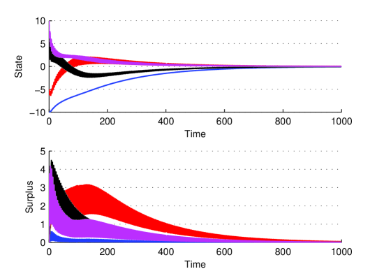
Figure 2: Convergence trajectories of states and surpluses obtained by applying the algorithm (3) for the topology in Fig. 1

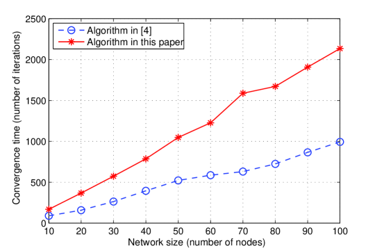
Figure 3: Convergence time comparison between the algorithm (3) and the one in [4]. Consider digraphs $\mathcal{G}_{n}$ with $n$ nodes derived from complete graphs with $n$ nodes by removing $n-2$ edges $(h,n)$, $h\in[2,n-1]$. Thus $\mathcal{G}_{n}$ are strongly connected, non-balanced digraphs, and we consider static $\mathcal{G}_{n}$ since the algorithm in [4] applies only to this case. For simplicity choose $a_{ij}=b_{ij}=1/n$ and $\epsilon_{i}=1/(2n)$. Run both algorithms on digraphs $\mathcal{G}_{n}$ with different $n$, and with initial states $x_{i}(0)$ randomly selected from $[-50,50]$, initial surpluses $s_{i}(0)=0$. Find the convergence times $t$ to be the minimum times when $||(x(t),s(t))-(x_{a}\textbf{1},0)||_{1}<0.05$, and each sample point on the displayed curves is the average convergence time of $50$ algorithm executions. Comparing the two curves we see that the convergence time of algorithm (3) is approximately twice as much as the one in [4], which is due to the former’s enforcement on nonnegative surpluses that produces undesirable switchings.

We provide a numerical example to illustrate the convergence result of the algorithm (3). Consider the periodically time-varying digraph $\mathcal{G}(k)=(\mathcal{V},\mathcal{E}(k))$, with period $\mathcal{K}=4$, displayed in Fig. 1. No single digraph is strongly connected, but $\mathcal{G}(k)$ is jointly strongly connected. For simplicity, we apply the algorithm (3) by choosing the parameters and weights to be constant: $\epsilon_{h}=a_{ij}=b_{ij}=1/4$ for all agents $h$ and all edges $(j,i)$. It is easily verified that this choice satisfies the requirements (P1)-(P3).

For the initial state $x(0)=[-10\ \-5\ 5\ 10]^{T}$ and the initial surplus $s(0)=0$, the state and surplus trajectories are displayed in Fig. 2. Observe that every state converges to the desired average $0$, and every surplus is always nonnegative and vanishes eventually. Also we see that there are considerable switchings in both states and surpluses due to the enforcement of nonnegative surpluses, which may undesirably slow down the convergence speed. Indeed, in a simulation study displayed in Fig. 3, we compare the algorithm (3) to the one in [4] (the latter poses no restriction on nonnegative surpluses), and find that the convergence time of algorithm (3) is approximately twice as much as the one in [4] for a class of digraphs. An important future study then would be to find appropriate (possibly time-varying) values of the parameters and weights so as to reduce switchings and accelerate convergence.

VI Conclusions

We have proposed a new surplus-based algorithm which enables networks of agents to achieve uniform average consensus on general time-varying digraphs that vary in some deterministic fashion. Our derived graphical condition does not require balanced or symmetric network topologies, and is hence more general than those previously reported in the literature. Future research will target convergence speed analysis of the algorithm as well as the design of fast surplus-based averaging algorithms.

References

- [1] D. P. Bertsekas and J. N. Tsitsiklis, Parallel and Distributed Computation: Numerical Methods. Prentice-Hall, 1989.
- [2] R. Olfati-Saber and R. M. Murray, “Consensus problems in networks of agents with switching topology and time-delays,” IEEE Trans. Autom. Control, vol. 49, no. 9, pp. 1520–1533, 2004.
- [3] L. Xiao and S. Boyd, “Fast linear iterations for distributed averaging,” Systems & Control Letters, vol. 53, pp. 65–78, 2004.
- [4] K. Cai and H. Ishii, “Average consensus on general strongly connected digraphs,” Automatica, vol. 48, no. 11, pp. 2750–2761, 2012. Also in Proc. 50th IEEE Conf. on Decision and Control and European Control Conf., pp. 1956-1961, 2011.
- [5] ——, “Quantized consensus and averaging on gossip digraphs,” IEEE Trans. Autom. Control, vol. 56, no. 9, pp. 2087–2100, 2011.
- [6] ——, “Average consensus on arbitrary strongly connected digraphs with dynamic topologies,” in Proc. American Control Conf., no. 14-19, Montreal, Canada, 2012.
- [7] L. Moreau, “Stability of multi-agent systems with time dependent communication links,” IEEE Trans. Autom. Control, vol. 50, no. 2, pp. 169–182, 2005.
- [8] Z. Lin, Distributed Control and Analysis of Coupled Cell Systems. VDM Verlag, 2008.
- [9] J. M. Hendrickx and J. N. Tsitsiklis, “Convergence of type-symmetric and cut-balanced consensus seeking systems,” IEEE Trans. Autom. Control, vol. 58, no. 1, pp. 214–218, 2013.
- [10] M. Franceschelli, A. Giua, and C. Seatzu, “Distributed averaging in sensor networks based on broadcast gossip algorithms,” IEEE Sensors J., vol. 11, no. 3, pp. 808–817, 2011.
- [11] F. Benezit, V. Blondel, P. Thiran, J. Tsitsiklis, and M. Vetterli, “Weighted gossip: distributed averaging using non-doubly stochastic matrices,” in Proc. IEEE Int. Symposium on Information Theory, Austin, TX, 2010, pp. 1753–1757.
- [12] A. D. Dominguez-Garcia and C. N. Hadjicostis, “Distributed matrix scaling and application to average consensus in directed graphs,” IEEE Trans. Autom. Control, no. 9, to appear, 2013. Also in Proc. 50th IEEE Conf. on Decision and Control and European Control Conf., pp. 2124-2129, 2011.
- [13] B. Gharesifard and J. Cortés, “Distributed strategies for generating weight-balanced and doubly stochastic digraphs,” European J. of Control, vol. 18, no. 6, pp. 539–557, 2012. Also arXiv:0911.0232v4 [math.OC].
- [14] W. Ren and R. W. Beard, Distributed Consensus in Multi-vehicle Cooperative Control: Theory and Applications. Springer-Verlag, 2008.
- [15] J. Liu, B. D. O. Anderson, M. Cao, and A. S. Morse, “Analysis of accelerated gossip algorithms,” in Proc. 48th IEEE Conf. on Decision and Control, Shanghai, China, 2009, pp. 871–876.
- [16] H. K. Khalil, Nonlinear Systems. 3rd ed., Prentice-Hall, 2002.