Handelman’s hierarchy for the maximum stable set problem

Abstract

The maximum stable set problem is a well-known NP-hard problem in combinatorial optimization, which can be formulated as the maximization of a quadratic square-free polynomial over the (Boolean) hypercube. We investigate a hierarchy of linear programming relaxations for this problem, based on a result of Handelman showing that a positive polynomial over a polytope with non-empty interior can be represented as conic combination of products of the linear constraints defining the polytope. We relate the rank of Handelman’s hierarchy with structural properties of graphs. In particular we show a relation to fractional clique covers which we use to upper bound the Handelman rank for perfect graphs and determine its exact value in the vertex-transitive case. Moreover we show two upper bounds on the Handelman rank in terms of the (fractional) stability number of the graph and compute the Handelman rank for several classes of graphs including odd cycles and wheels and their complements. We also point out links to several other linear and semidefinite programming hierarchies.

1 Introduction

In this paper we consider the maximum stable set problem, a well-known NP-hard problem in combinatorial optimization. We study a global optimization approach, based on reformulating the maximum stability number $\alpha(G)$ of a graph $G$ as the maximum of a (square-free) quadratic polynomial on the hypercube $[0,1]^{n}$, as in relation (2) below. We investigate a hierarchy of linear programming bounds, motivated by a result of Handelman DH88 for certifying positive polynomials on the hypercube. While several other linear or semidefinite programming hierarchical relaxations exist, a main motivation for focusing on the relaxations of Handelman type is that they appear to be easier to analyze. Indeed, explicit error bounds have been given for general polynomials in KL10 and sharper bounds that apply at any order of relaxation have been given in PH11 ; PH12 for square-free quadratic polynomials, as we will recall below. Moreover, we focus on the maximum stable set problem, since it is fundamental in the sense that any polynomial optimization problem on the hypercube can be transformed into a maximum stable set problem using the so-called conflict graph BB89 . Moreover, Cornaz and Jost CJ08 give a direct explicit reformulation for the graph coloring problem as an instance of maximum stable set problem.

Algebraic approaches for the maximum stable set problem have been long studied; see e.g. the early work of Lovász Lov94 and the more recent work of De Loera et al. LLMO09 , where Hilbert’s Nullstellensatz plays a central role to show the non-existence of a solution to a system of polynomial equations. For instance, LLMO09 uses the polynomial system: $x_{i}-x_{i}^{2}=0$ for $i\in V(G)$, $x_{i}x_{j}=0$ for $ij\in E(G)$ and $\sum_{i\in V(G)}x_{i}=k$, to encode the question of existence of a stable set of size $k$ in $G$. For $k\geq\alpha(G)+1$ this sytem is infeasible and LLMO09 gives an explicit Nullstellensatz certificate certifying this and such certificates can be searched using Gaussian elimination (or linear programming). Other algebraic approaches, based on finding conditions for expressing positivity of polynomials, permit to construct upper bounds for the stability number. Depending on the type of positivity certificates one finds linear or semidefinite programming bounds (cf. e.g. GPT ; KP02 ; Las02 ; Lau03 ; PVZ12 ; SA90 ). In this paper we focus on the Handelman approach, where one searches for positivity certificates obtained as conic combinations of the linear polynomials defining the hypercube. This approach for the maximum stable set problem was initiated by Park and Hong PH12 (also in PH11 for the maximum cut problem) and we will extend several of their results.

We now introduce the Handelman hierarchy for polynomial optimization problems and recall some known results for optimization on the standard simplex and on the hypercube.

1.1 Polynomial optimization

Given polynomials $p,g_{1},\ldots,g_{m}\in{\mathbb{R}}[x]$ in $n$ variables $x=(x_{1},\ldots,x_{n})$, we consider the following polynomial optimization problem:

$$p_{\text{\rm max}}=\max\ p(x)\ \text{ s.t. }\ x\in K=\{x\in{\mathbb{R}}^{n}:g_{1}(x)\geq 0,\ldots,g_{m}(x)\geq 0\},$$ (1)

which asks to maximize $p$ over the basic closed semialgebraic set $K$. This is an NP-hard problem, since it contains e.g. the maximum stable set problem and the maximum cut problem, two well-known NP-hard problems. Both problems can indeed be formulated as instances of (1) where $p$ is a quadratic polynomial and $K=[0,1]^{n}$ is the hypercube. Namely, given a graph $G=(V,E)$, the maximum cardinality $\alpha(G)$ of a stable set in $G$ can be computed via the polynomial optimization problem:

$$\alpha(G)=\max_{x\in[0,1]^{n}}\sum_{i\in V}x_{i}-\sum_{ij\in E}x_{i}x_{j},$$ (2)

and the maximum cardinality of a cut in $G$ can be computed via the following problem:

$${\rm mc}(G)=\max_{x\in[0,1]^{n}}\sum_{i\in V}\deg(i)x_{i}-2\sum_{ij\in E}x_{i}x_{j},$$ (3)

where $\deg(i)$ denotes the degree of node $i$ in $G$. See e.g. PH11 ; PH12 and Proposition 2 below.

With $\mathscr{P}(K)$ denoting the set of real polynomials that are nonnegative on the set $K$, problem (1) can be rewritten as

$$p_{\text{\rm max}}=\min\ \lambda\ \ \text{\rm{s.t.}}\ \ \lambda-p\in\mathscr{P}(K).$$

A popular approach in the recent years is based on replacing the (hard to test) positivity condition $\lambda-p\in\mathscr{P}(K)$ by a tractable, sufficient condition for positivity. For instance, one may search for positivity certificates of the form $\lambda-p=\sum_{\alpha\in{\mathbb{N}}^{m}}c_{\alpha}g_{1}^{\alpha_{1}}\cdots g_{m}^{\alpha_{m}}$, where the multipliers $c_{\alpha}$ are nonnegative scalars, which leads to the so-called Handelman hierarchy of linear programming relaxations for (1). When the $g_{j}$’s are linear polynomials and $K$ is a polytope, the asymptotic convergence to $p_{\text{\rm max}}$ is guaranteed by the following result of Handelman DH88 .

Theorem 1.1

DH88 Assume that $g_{1},\dots,g_{m}\in{\mathbb{R}}[x]$ are linear polynomials and that the set

$$K=\{x\in{\mathbb{R}}^{n}:g_{1}(x)\geq 0,\dots,g_{m}(x)\geq 0\}$$ (4)

is compact and has a non-empty interior. Then for any polynomial $p\in{\mathbb{R}}[x]$ strictly positive on $K$, $p$ can be written as $\sum_{\alpha\in{\mathbb{N}}^{m}}c_{\alpha}g_{1}^{\alpha_{1}}\cdots g_{m}^{\alpha_{m}}$ for some nonnegative scalars $c_{\alpha}$.

In the case of the hypercube $K=\{x\in{\mathbb{R}}^{n}:0\leq x_{i}\leq 1\ \forall i\in[n]\}$, this result was shown already earlier by Krivine Kr64 .

Alternatively, one may search for positivity certificates of the form $\sum_{\alpha\in{\mathbb{N}}^{m}}s_{\alpha}g_{1}^{\alpha_{1}}\cdots g_{m}^{\alpha_{m}}$ (or of the simpler form $s_{0}+\sum_{j=1}^{m}s_{j}g_{j}$), where the multipliers $s_{\alpha}$ (or $s_{0},s_{j}$) are now sums of squares of polynomials. This leads to the Lasserre hierarchy of semidefinite programming relaxations for (1), whose asymptotic convergence is guaranteed for $K$ compact (satisfying an additional Archimedean condition) by results of real algebraic geometry (see e.g. Las02 ; Lau09 ).

Although the Lasserre hierarchy is stronger, it is more difficult to analyze and computationally more expensive as it relies on semidefinite programming. This motivates the study of the linear programming based Handelman hierarchy which is generally easier to analyze, and might yet provide some insightful information, also for the SDP based hierarchies which dominate it. Some results have been proved on the convergence rate in the case when $K$ is the standard simplex or the hypercube $[0,1]^{n}$, which we recall below.

1.2 The Handelman hierarchy

We now present a hierarchy of linear relaxations for problem (1), which is motivated by the above mentioned result of Handelman for certifying positivity of polynomials on a semialgebraic set $K$ of the form (4). We let $g$ denote the set of polynomials $g_{1},\ldots,g_{m}$. For an integer $t\geq 1$, define the Handelman set of order t as

$${\mathcal{H}}_{t}(g):=\left\{\sum_{\alpha\in{\mathbb{N}}^{m}:|\alpha|\leq t}c_{\alpha}g^{\alpha}:c_{\alpha}\geq 0\right\}$$

and the corresponding Handelman bound of order $t$ as

$$p_{\text{\rm han}}^{(t)}:=\inf\{\lambda:\lambda-p\in{\mathcal{H}}_{t}(g)\}.$$

Clearly, any polynomial in ${\mathcal{H}}_{t}(g)$ is nonnegative on $K$ and one has the following chain of inclusions:

$$\mathcal{H}_{1}(g)\subseteq\ldots\subseteq\mathcal{H}_{t}(g)\subseteq{\mathcal{H}}_{t+1}(g)\subseteq\ldots\subseteq\mathscr{P}(K),$$

giving the chain of inequalities: $p_{\text{\rm max}}\leq p_{\text{\rm han}}^{(t+1)}\leq p_{\text{\rm han}}^{(t)}\leq\dots\leq p_{\text{\rm han}}^{(1)}$ for $t\geq 1$. When $K$ is a polytope with non-empty interior and $g_{1},\ldots,g_{m}$ are linear polynomials, the asymptotic convergence of the bounds $p_{\text{\rm han}}^{(t)}$ to $p_{\text{\rm max}}$ as the order $t$ increases is guaranteed by Theorem 1.1 above. We mention two cases where results are known about the quality of the Handelman bounds, when $K$ is the standard simplex or the hypercube.

Application to optimization on the simplex.

We first consider the case when $K=\Delta$ is the standard simplex $\Delta=\{x\in{\mathbb{R}}^{n}:x\geq 0,\ \sum_{i=1}^{n}x_{i}=1\}.$ Define the polynomial $\sigma=\sum_{i=1}^{n}x_{i}$. Let $\langle 1-\sigma\rangle$ denote the ideal in ${\mathbb{R}}[x]$ generated by the polynomial $1-\sigma$ and, for an integer $t$, let $\langle 1-\sigma\rangle_{t}$ denote its truncation at degree $t$, consisting of all polynomials of the form $u(1-\sigma)$ where $u\in{\mathbb{R}}[x]$ has degree at most $t-1$. Moreover, let ${\mathbb{R}}_{+}[x]$ denote the set of polynomials with nonnegative coefficients and ${\mathbb{R}}_{+}[x]_{t}$ its subset consisting of polynomials of degree at most $t$. With $g$ standing for the set of polynomials $x_{1},\ldots,x_{n},\pm(1-\sigma)$, one can easily see that the Handelman set of order $t$ is given by

$${\mathcal{H}}_{t}(g)={\mathbb{R}}_{+}[x]_{t}+\langle 1-\sigma\rangle_{t}.$$

Suppose we wish to maximize $p$ over $\Delta$, where $p\in{\mathbb{R}}[x]$ is a polynomial of degree $d$ which we can assume to be homogeneous without loss of generality. It turns out that the corresponding Handelman bound $p_{\text{\rm han}}^{(t)}$ coincides with the LP bound studied in Fay03 ; KLP06 , based on Pólya’s positivity certificate and defined as follows:

$$\inf\{\lambda:(\lambda\sigma^{d}-p)\sigma^{t-d}\in{\mathbb{R}}_{+}[x]\}.$$

This follows from the following lemma (based on similar arguments as in KLP05 ).

Lemma 1

Let $p$ be a homogeneous polynomial of degree $d$, $\lambda\in{\mathbb{R}}$ and an integer $t\geq d$. Then, $\lambda-p\in{\mathbb{R}}_{+}[x]_{t}+\langle 1-\sigma\rangle_{t}$ if and only if $(\lambda\sigma^{d}-p)\sigma^{t-d}\in{\mathbb{R}}_{+}[x].$ Therefore, $p_{\text{\rm han}}^{(t)}=\inf\{\lambda:(\lambda\sigma^{d}-p)\sigma^{t-d}\in{\mathbb{R}}_{+}[x]\}.$

Proof

Assume $(\lambda\sigma^{d}-p)\sigma^{t-d}\in{\mathbb{R}}_{+}[x].$ By writing $\sigma=1+(\sigma-1)$ and expanding the products $\sigma^{d}$ and $\sigma^{t}$, one obtains a decomposition of $\lambda-p$ in ${\mathbb{R}}_{+}[x]_{t}+\langle 1-\sigma\rangle_{t}$. Conversely, assume that $\lambda-p\in{\mathbb{R}}_{+}[x]_{t}+\langle 1-\sigma\rangle_{t}$. This implies that $\lambda\sigma^{d}-p=f+u(1-\sigma)$, where $f\in{\mathbb{R}}_{+}[x]_{t}$ and $u\in{\mathbb{R}}[x]_{t-1}$. By evaluating both sides at $x/\sigma$ and multiplying throughout by $\sigma^{t}$, we obtain that $\sigma^{t-d}(\lambda\sigma^{d}-p)=f(x/\sigma)\sigma^{t}\in{\mathbb{R}}_{+}[x]$, since $f$ has degree at most $t$. ∎

Therefore the results of de Klerk, Laurent and Parrilo KLP06 apply and give the following error estimates for the Handelman bound of order $t\geq d$:

$$p_{\text{\rm han}}^{(t)}-p_{\text{\rm max}}\leq d^{d}{2d-1\choose d}\frac{{d\choose 2}}{t-{d\choose 2}}(p_{\text{\rm max}}-p_{\text{\rm min}}),$$

where $p_{\text{\rm min}}$ is the minimum value of $p$ over the simplex $\Delta$.

Application to optimization on the hypercube.

We now turn to the case when $K=[0,1]^{n}$ is the hypercube. Using Bernstein approximations, de Klerk and Laurent KL10 have shown the following error estimates for the Handelman hierarchy. If $p$ is a polynomial of degree $d$ and $r\geq 1$ is an integer then the Handelman bound of order $t=rn$ satisfies:

$$p_{\text{\rm han}}^{(rn)}-p_{\text{\rm max}}\leq{L(p)\over r}{d+1\choose 3}n^{d},$$

setting $L(p)=\max_{\alpha}{\alpha!\over|\alpha|!}|p_{\alpha}|$. In the quadratic case a better estimate can be shown.

Theorem 1.2

(KL10, , Proposition 3.2) Let $p=x^{T}Ax+b^{T}x$ be a quadratic polynomial. For any integer $r\geq 1$,

$$p_{\text{\rm han}}^{(rn)}-p_{\text{\rm max}}\leq\frac{-\sum_{i:A_{ii}<0}A_{ii}}{r}.$$

We observe that the above results hold only for relaxations of order $t\geq n$. Moreover, if $p$ is a square-free quadratic polynomial (i.e., $A_{ii}=0$ for all $i$), then equality $p_{\text{\rm max}}=p_{\text{\rm han}}^{(n)}$ holds and the Handelman relaxation of order $n$ gives the exact value $p_{\text{\rm max}}$. This is consistent with the fact that a square-free polynomial takes the same maximum value on the hypercube $[0,1]^{n}$ as on the Boolean hypercube $\{0,1\}^{n}$.

Using a combinatorial version of Bernstein approximations, Park and Hong PH12 can analyze the Handelman bound of any order $t\leq n$, in the quadratic square-free case. They show the following result (see Section 2.2 for a proof).

Theorem 1.3

PH12 Let $p=x^{T}Ax+b^{T}x$ be a quadratic polynomial which is square-free, i.e., $A_{ii}=0$ for all $i\in[n]$. Assume moreover that $A_{ij}\leq 0$ for all $i\neq j\in[n]$. Then, for any integer $2\leq t\leq n$,

$$p_{\text{\rm han}}^{(t)}\leq{n\over t}p_{\text{\rm max}}.$$

1.3 Contribution of the paper

The error analysis from Theorem 1.3 applies in particular to the bounds obtained by applying the Handelman hierarchy to the formulation (2) of the maximum stable set problem and to the formulation (3) of the maximum cut problem PH11 ; PH12 , whereas no error analysis is known for other (potentially stronger) linear or semidefinite programming hierarchies. This is one of the main motivations for investigating the Handelman hierarchy. Park and Hong PH11 ; PH12 give some preliminary results on the rank of the Handelman hierarchy, defined as the smallest order $t$ for which the Handelman bound is exact. In particular, they show that when applied to both the maximum stable set and cut problems, the Handelman hierarchy has rank 2 for bipartite graphs and rank 3 for odd cycles (in the unweighted case) and they ask whether these results extend to weighted graphs. We give an affirmative answer to this open question.

The paper is devoted to the Handelman hierarchy applied to the formulation (2) of the maximum stable set problem. In particular, we bound the rank of the Handelman hierarchy for several graph classes, including perfect graphs, odd cycles and wheels, and their complements, in the general weighted case. Moreover we show that the Handelman bound of order 2 is equal to the fractional stability number (see Theorem 3.1). We also prove two different upper bounds for the Handelman rank for a weighted graph, one in terms of the (unweighted) stability number and one in terms of the weighted stability and fractional stability numbers (see Theorem 3.2 and Corollary 4). For this we develop the following two main tools.

First we show a relationship between the Handelman bound of order $t$ and the fractional $t$-clique cover number, at any given order $t\geq 2$, by constructing explicit decompositions in the Handelman set of order $t$ from clique covers. At the smallest order $t=2$, we show that both bounds coincide, which implies that the Handelman bound of order 2 coincides with the fractional stable set number. Additionally this allows us to upper bound the Handelman rank of any perfect graph $G$ by its maximum clique size, with equality when $G$ is vertex-transitive (Proposition 5).

Second we observe a simple identity for square-free polynomials (Lemma 5), which can be used to relate the algebraic operation of setting a variable to 0 (resp. to 1) to the graph operation of deleting a node (resp., deleting a node and its neighbours). This technique permits to relate the Handelman rank with structural properties of graphs and can be applied to show the upper bounds and to deal e.g. with odd cycles and odd wheels.

In addition, for the maximum cut problem, we clarify how the Handelman hierarchy applies to the formulation (3) and show that it can be reformulated as optimization over a polytope defined by an explicit subset of valid inequalities for the cut polytope; as an application we find again several results of PH11 ; PH12 (see Section 5).

More specifically the paper is organized as follows. In Section 2 we present some preliminary results about square-free polynomials and the Handelman hierarchy. In particular we prove the error bound from Theorem 1.3 (for polynomials of arbitrary degree) and we introduce the Handelman hierarchy for the maximum stable set problem. Section 3 contains our new results. In Section 3.1 we show a relation to fractional clique coverings and we show that the Handelman bound of order 2 is equal to the fractional stability number. Section 3.2 contains the two new upper bounds for the Handelman rank, in Section 3.3 we determine the Handelman rank of several classes of graphs, and in Section 3.4 we study the behaviour of the Handelman rank under some graph operations like edge deletion and clique sums. In Section 4 we point out links to the linear or semidefinite programming hierarchies of Sherali-Adams, Lasserre, Lovász-Schrijver, and de Klerk-Pasechnik. In Section 5 we give an explicit formulation for the Handelman hierarchy applied to the maximum cut problem in terms of valid inequalities of the cut polytope.

1.4 Notation

For an integer $n\geq 1$, we set $[n]:=\{1,2\dots,n\}$. Given a finite set $V$ and an integer $t$, ${\mathcal{P}}(V)$ denotes the collection of all subsets of $V$, ${\mathcal{P}}_{t}(V):=\{I\subseteq V:|I|\leq t\}$, and ${\mathcal{P}}_{=t}(V):=\{I\subseteq V:|I|=t\}$. The support of $x\in{\mathbb{R}}^{n}$ is the set $\{i\in[n]:x_{i}\neq 0\}$. For $x\in{\mathbb{R}}^{n}$ and $S\subseteq[n]$, $x(S)=\sum_{i\in S}x_{i}$. We let $e$ denote the all-ones vector in ${\mathbb{R}}^{n}$ and $e_{1},\dots,e_{n}$ denote the standard unit vectors in ${\mathbb{R}}^{n}$. For a subset $I\subseteq[n]$, $\chi^{I}\in\{0,1\}^{n}$ denotes its characteristic vector. The space of symmetric $n\times n$ matrices is denoted as $\mathcal{S}_{n}$. A matrix $A\in\mathcal{S}_{n}$ is positive semidefinite (resp., copositive) if $x^{T}Ax\geq 0$ for all $x\in{\mathbb{R}}^{n}$ (resp., $x^{T}Ax\geq 0$ for all $x\geq 0$). Then, $\mathcal{S}_{n}^{+}$ denotes the positive semidefinite cone, consisting of all positive semidefinite matrices in $\mathcal{S}_{n}$, and ${\mathcal{C}}_{n}$ is the copositive cone, consisting of all copositive matrices.

Let ${\mathbb{R}}[x]={\mathbb{R}}[x_{1},\dots,x_{n}]$ denote the ring of multivariate polynomials in $n$ variables with real coefficients. Monomials in ${\mathbb{R}}[x]$ are denoted as $x^{\alpha}=x_{1}^{\alpha_{1}}\cdots x_{n}^{\alpha_{n}}$ for $\alpha\in{\mathbb{N}}^{n}$, with degree $|\alpha|:=\sum_{i=1}^{n}\alpha_{i}$. For a polynomial $p=\sum_{\alpha\in{\mathbb{N}}^{n}}p_{\alpha}x^{\alpha}$, its degree is defined as ${\rm deg}(p):=\max_{\alpha|p_{\alpha}\neq 0}|\alpha|$. For an integer $t$, ${\mathbb{R}}[x]_{t}$ denotes the subspace of polynomials with degree at most $t$. The monomial $x^{\alpha}$ is said to be square-free (aka multilinear) if $\alpha\in\{0,1\}^{n}$ and a polynomial $p$ is square-free if all its monomials are square-free. For $I\subseteq[n]$, we use the notation $x^{I}=\prod_{i\in I}x_{i}$. Hence a square-free polynomial can be written as $\sum_{I\subseteq[n]}p_{I}x^{I}$. Given a subset $S\subseteq{\mathbb{R}}^{n}$, we say that $p\in{\mathbb{R}}[x]$ is positive (resp., nonnegative) on $S$ when $p(x)>0$ (resp., $p(x)\geq 0$) for all $x\in S$. Given $g_{1},\dots,g_{m}\in{\mathbb{R}}[x]$ and $s\in{\mathbb{N}}^{m}$, we often use the notation $g^{s}=g_{1}^{s_{1}}\cdots g_{m}^{s_{m}}$, with $g^{0}=1$. The ideal generated by a set of polynomials $g_{1},\ldots,g_{m}\in{\mathbb{R}}[x]$ is the set, denoted as $\langle g_{1},\ldots,g_{m}\rangle$, consisting of all polynomials of the form $\sum_{j=1}^{m}u_{j}g_{j}$ where $u_{j}\in{\mathbb{R}}[x]$.

Given a graph $G=(V,E)$, $\overline{G}=(V,\overline{E})$ denotes its complementary graph whose edges are the pairs of distinct nodes $i,j\in V(G)$ with $ij\notin E$. Throughout we also set $V=V(G)$, $E=E(G)$ and we often assume $V(G)=[n]$. $K_{n}$ denotes the complete graph and $C_{n}$ the circuit on $n$ nodes. A set $S\subseteq V$ is stable (or independent) if no two distinct nodes of $S$ are adjacent in $G$ and a clique in $G$ is a set of pairwise adjacent nodes. The maximum cardinality of a stable set (resp., clique) in $G$ is denoted by $\alpha(G)$ (resp., $\omega(G)$); thus $\omega(G)=\alpha(\overline{G})$. The chromatic number $\chi(G)$ is the minimum number of colors needed to color the nodes of $G$ in such a way that adjacent nodes receive distinct colors. For a node $i\in V$, $G-i$ denotes the graph obtained by deleting node $i$ from $G$, and $G\ominus i$ denotes the graph obtained from $G$ by removing $i$ as well as the set $N(i)$ of its neighbours. For $U\subseteq V$, $G\backslash U$ denotes the graph obtained by deleting all nodes of $U$. For an edge $e\in E$, let $G\backslash e$ denote the graph obtained by deleting edge $e$ from $G$, and let $G/e$ denote the graph obtained from $G$ by contracting edge $e$. Consider two graphs $G_{1}=(V_{1},E_{1})$ and $G_{2}=(V_{2},E_{2})$ such that $V_{1}\cap V_{2}$ is a clique of cardinality $t$ in both $G_{1}$ and $G_{2}$. Then the graph $G=(V_{1}\cup V_{2},E_{1}\cup E_{2})$ is called the clique $t$-sum of $G_{1}$ and $G_{2}$.

2 Preliminaries

2.1 Maximization of square-free polynomials over the hypercube

In this section we group some observations about the Handelman hierarchy when it is applied to the problem of maximizing a square-free polynomial $p$ over the hypercube:

$$p_{\text{\rm max}}=\max_{x\in[0,1]^{n}}p(x).$$

In what follows we let ${\mathcal{I}}$ denote the ideal generated by the polynomials $x_{i}^{2}-x_{i}$ for $i\in[n]$. Using the description of the hypercube by the inequalities: $x_{i}\geq 0,1-x_{i}\geq 0$ for $i\in[n]$, the corresponding Handelman set of order $t$ reads:

$$\mathcal{H}_{t}=\left\{\sum_{\alpha,\beta\in{\mathbb{N}}^{n}:|\alpha+\beta|\leq t}c_{\alpha,\beta}x^{\alpha}(1-x)^{\beta}:c_{\alpha,\beta}\geq 0\right\}.$$ (5)

We also consider the following subset consisting of all square-free polynomials in ${\mathcal{H}}_{t}$ involving only terms which do not lie in the ideal ${\mathcal{I}}$:

$$H_{t}:=\left\{\sum_{T\in{\mathcal{P}}_{t}(V),I\subseteq T}c_{T,I}x^{I}(1-x)^{T\setminus I}:c_{T,I}\geq 0\right\}.$$ (6)

Clearly, in the definition of $H_{t}$, we can restrict without loss of generality to sets $T\in{\mathcal{P}}_{=t}(V)$. Indeed, if $T<t$, pick an element $k\in V\setminus T$ and elevate the degree of $x^{I}(1-x)^{T\setminus I}$ by writing $x^{I}(1-x)^{T\setminus I}=x^{I\cup\{k\}}(1-x)^{T\setminus I}+x^{I}(1-x)^{(T\setminus I)\cup\{k\}}$.

By construction, the Handelman bound $p_{\text{\rm han}}^{(t)}$ for the maximum value $p_{\text{\rm max}}$ of $p$ over $[0,1]^{n}$ is defined using the set ${\mathcal{H}}_{t}$ in (5). We now show that it can alternatively be defined using the subset $H_{t}$ in (6).

Proposition 1

Let $p\in{\mathbb{R}}[x]$ be a square-free polynomial. For any integer $t\geq 1$,

$$p_{\text{\rm han}}^{(t)}:=\inf\{\lambda:\lambda-p\in{\mathcal{H}}_{t}\}=\inf\{\lambda:\lambda-p\in H_{t}\}.$$

This result follows directly from Lemma 4 below, whose proof relies on the following Lemmas 2 and 3.

Lemma 2

If $p$ is a square-free polynomial and $p\in{\mathcal{I}}$, then $p=0$.

Proof

We use induction on the number $n$ of variables. In the case $n=1$, we have that $p=p_{0}+p_{1}x_{1}=f_{1}\cdot(x_{1}-x_{1}^{2})$, which implies $f_{1}=0$ and thus $p=0$ by looking at the degrees of both sides. Suppose now that the result holds for $n=k-1$. Let $p$ be a square-free polynomial in $k$ variables lying in the ideal ${\mathcal{I}}$. We can write $p$ as $p(x)=p_{0}(\underline{x})+x_{k}p_{1}(\underline{x})$, where $p_{0}$, $p_{1}$ are square-free in the $k-1$ variables $\underline{x}=(x_{1},\cdots,x_{k-1})$. Say, $p_{0}+x_{k}p_{1}=p=\sum_{i=1}^{k}f_{i}\cdot(x_{i}-x_{i}^{2})$ for some polynomials $f_{i}$. By setting $x_{k}=0$ we get: $p_{0}(\underline{x})=\sum_{i=1}^{k-1}f_{i}(\underline{x},0)(x_{i}-x_{i}^{2})$. As $p_{0}$ is square-free, we deduce using the induction assumption that $p_{0}=0$. Next, by setting $x_{k}=1$, we get: $p_{1}(\underline{x})=\sum_{i=1}^{k-1}f_{i}(\underline{x},1)(x_{i}-x_{i}^{2})$. As $p_{1}$ is square-free we deduce from the induction assumption that $p_{1}=0$. Thus we have shown that $p=0$. ∎

Lemma 3

Given $\alpha,\beta\in{\mathbb{N}}^{n}$, let $I=\{i\in[n]:\alpha_{i}\geq 1\}$ and $J=\{i\in[n]:\beta_{i}\geq 1\}$ denote their supports.

• If $I\cap J\neq\emptyset$ then $x^{\alpha}(1-x)^{\beta}$ belongs to ${\mathcal{I}}$.

• If $I\cap J=\emptyset$ then $x^{\alpha}(1-x)^{\beta}-x^{I}(1-x)^{J}$ belongs to ${\mathcal{I}}$.

Proof

(i) Say, $1\in I\cap J$. Then $x_{1}(1-x_{1})$ is a factor of $x^{\alpha}(1-x)^{\beta}$ and thus $x^{\alpha}(1-x)^{\beta}\in{\mathcal{I}}$.
(ii) The proof is based on using iteratively the following identities, for any $k\geq 2$:

$$x_{i}^{k}-x_{i}=(x_{i}^{2}-x_{i})(x_{i}^{k-2}+\cdots+x_{i}+1)\in{\mathcal{I}},$$

$$(1-x_{i})^{k}-(1-x_{i})=-x_{i}(1-x_{i})((1-x_{i})^{k-2}+\cdots+(1-x_{i})+1)\in{\mathcal{I}}.$$

Indeed, $x^{\alpha}(1-x)^{\beta}-x^{I}(1-x)^{J}=(x_{1}^{\alpha_{1}}-x_{1})\underline{x}^{\underline{\alpha}}(1-x)^{\beta}+x_{1}(\underline{x}^{\underline{\alpha}}(1-x)^{\beta}-\underline{x}^{I\setminus\{1\}}(1-x)^{J}),$ setting $\underline{x}=(x_{2},\cdots,x_{n})$ and $\underline{\alpha}=(\alpha_{2},\cdots,\alpha_{n})$. ∎

Lemma 4

Let $p$ be a square-free polynomial and $t\geq 1$ an integer. The following assertions are equivalent.

• $p\in{\mathcal{H}}_{t}$.

• $p\in H_{t}+{\mathcal{I}}$.

• $p\in H_{t}$.

Proof

(i) $\Longrightarrow$ (ii): Say, $p=\sum_{A}c_{\alpha,\beta}x^{\alpha}(1-x)^{\beta}$ where $c_{\alpha,\beta}\geq 0$. Group in the polynomial $p_{0}=\sum_{A_{0}}c_{\alpha,\beta}x^{\alpha}(1-x)^{\beta}$ all the terms of $p$ where the supports of $\alpha$ and $\beta$ are not disjoint. Let $S_{\alpha}$ denote the support of $\alpha$. Then, we have:

$$p=p_{0}+\sum_{A\setminus A_{0}}c_{\alpha,\beta}(x^{\alpha}(1-x)^{\beta}-x^{S_{\alpha}}(1-x)^{S_{\beta}})+\sum_{A\setminus A_{0}}c_{\alpha,\beta}x^{S_{\alpha}}(1-x)^{S_{\beta}}.$$

By Lemma 3, the first two sums lie in ${\mathcal{I}}$ and the last sum lies in $H_{t}$ and thus $p\in H_{t}+{\mathcal{I}}$.
The implication (ii) $\Longrightarrow$ (iii) follows from Lemma 2 and (iii) $\Longrightarrow$ (i) follows from the inclusion $H_{t}\subseteq{\mathcal{H}}_{t}$. ∎

As an application of Lemma 2, we also find the following representation for square-free polynomials, which corresponds to the fact that the polynomials $\{x^{I}(1-x)^{[n]\setminus I}:I\subseteq[n]\}$ form a basis of the vector space of square-free polynomials.

Corollary 1

Any square-free polynomial $p$ can be written as

$$p=\sum_{I\subseteq[n]}p(\chi^{I})x^{I}(1-x)^{[n]\setminus I}.$$ (7)

Therefore, if $p(x)\geq 0$ for all $x\in\{0,1\}^{n}$, then $p\in H_{n}$.

Proof

The polynomial $p-\sum_{I\subseteq[n]}p(\chi^{I})x^{I}(1-x)^{[n]\setminus I}$ is square-free and vanishes on $\{0,1\}^{n}$. Hence it belongs to the ideal ${\mathcal{I}}$ and thus it is identically zero, by Lemma 2. ∎

In particular, as the polynomial $p_{\text{\rm max}}-p$ is nonnegative on the hypercube, we find again the convergence: $p_{\text{\rm han}}^{(n)}=p_{\text{\rm max}}$ of the Handelman hierarchy in $n$ steps, when $p$ is square-free. We mention another application which we will use later in the paper.

Lemma 5

Let $f$ be a square-free polynomial in $n$ variables $x=(x_{1},\ldots,x_{n})=(\underline{x},x_{n})$, setting $\underline{x}=(x_{1},x_{2}\dots,x_{n-1})$. Then, one has

$$f(x)=(1-x_{n})f(\underline{x},0)+x_{n}f(\underline{x},1).$$

Proof

Using (7) (and splitting the sum into two sums depending whether $I$ contains $n$ or not), we can write $f(x)$ as $f(x)=x_{n}f_{1}(\underline{x})+(1-x_{n})f_{2}(\underline{x})$. By evaluating $f$ at $(\underline{x},0)$ and $(\underline{x},1)$, we obtain that $f(\underline{x},0)=f_{2}(\underline{x})$ and $f(\underline{x},1)=f_{1}(\underline{x})$, which gives the result. ∎

2.2 Error bound of Handelman hierarchy

We now extend the result of Theorem 1.3 analyzing the Handelman bound of any order $t\leq n$ to polynomials of arbitrary degree.

Theorem 2.1

Let $p=\sum_{J\subseteq[n]}p_{J}x^{J}$ be a square-free polynomial with $p(0)=0$. For any integer $t$ satisfying $\text{\rm deg}(p)\leq t\leq n$, we have

$$p_{\text{\rm han}}^{(t)}\leq{n\over t}p_{\text{\rm max}}+\sum_{J\subseteq[n]:|J|\geq 2,p_{J}>0}p_{J}\lambda_{J},$$

setting

$$\lambda_{J}=\left({n-1\choose t-1}-{n-|J|\choose t-|J|}\right)/{n-1\choose t-1}\ \ \text{ for }J\subseteq[n].$$

Hence, if $p_{J}\leq 0$ for all $J\subseteq[n]$ with $|J|\geq 2$, then

$$p_{\text{\rm han}}^{(t)}\leq{n\over t}p_{\text{\rm max}}.$$

Proof

The proof is along the same lines as the proof of (PH12, , Proposition 3.2) and uses the following ‘combinatorial’ Bernstein approximation of $p$, defined as

$$B_{t}(p):=\sum_{T\in{\mathcal{P}}_{=t}([n])}\sum_{I\subseteq T}p(\chi^{I})x^{I}(1-x)^{T\backslash I}.$$

One can check that

$$B_{t}(x^{J})=\sum_{T\in{\mathcal{P}}_{=t}([n]):J\subseteq T}\sum_{I:J\subseteq I\subseteq T}x^{I}(1-x)^{T\backslash I}=\sum_{T\in{\mathcal{P}}_{=t}([n]):J\subseteq T}x^{J}={n-|J|\choose t-|J|}x^{J}$$

for any $J\subseteq[n]$. Hence, the Bernstein approximation of $p=\sum_{J\subseteq[n]}p_{J}x^{J}$ reads

$$B_{t}(p)=\sum_{J:J\subseteq[n],|J|\leq t}p_{J}{n-|J|\choose t-|J|}x^{J}.$$ (8)

Now we divide throughout by $n-1\choose t-1$ and add to both sides of (8) the quantity $\sum_{J}p_{J}\lambda_{J}x^{J}$ to get

$${B_{t}(p)\over{n-1\choose t-1}}+\sum_{J}p_{J}\lambda_{J}x^{J}=p.$$

As $B_{t}(1)={n\choose t}={n\over t}{n-1\choose t-1}$, this gives ${n\over t}p_{\text{\rm max}}={B_{t}(p_{\text{\rm max}})\over{n-1\choose t-1}}$ and thus we obtain

$${n\over t}p_{\text{\rm max}}-p={B_{t}(p_{\text{\rm max}}-p)\over{n-1\choose t-1}}-\sum_{J}\lambda_{J}p_{J}x^{J}.$$ (9)

As the polynomial $p_{\text{\rm max}}-p$ is nonnegative over $\{0,1\}^{n}$, it follows from the definition of the Bernstein operator that

$$B_{t}(p_{\text{\rm max}}-p)=\sum_{T\in{\mathcal{P}}_{=t}([n])}\sum_{I\subseteq T}(p_{\max}-p(\chi^{I}))x^{I}(1-x)^{T\backslash I}\in H_{t}.$$

As $\lambda_{J}\geq 0$ for all $J$, after moving the terms $p_{J}\lambda_{J}x^{J}$ with $p_{J}>0$ to the left hand side of (9), we obtain the claimed inequalities. ∎

2.3 The maximum stable set problem

Let $G=(V,E)$ be a graph and let $w\in{\mathbb{R}}^{V}_{+}$ be weights assigned to the nodes of $G$. The maximum stable set problem is to determine the maximum weight $w(S)=\sum_{i\in S}w_{i}$ of a stable set $S$ in $G$, called the weighted stability number of $(G,w)$ and denoted as $\alpha(G,w)$. Let $\text{\rm ST}(G)$ denote the polytope in ${\mathbb{R}}^{V}$, defined as the convex hull of the characteristic vectors of the stable sets of $G$:

$$\text{\rm ST}(G):={\rm{conv}}\{\chi^{S}:S\subseteq V,\ \ \text{$S$ is a stable set in $G$}\},$$

called the stable set polytope of G. Hence, computing $\alpha(G,w)$ is a linear optimization problem over the stable set polytope:

$$\alpha(G,w)=\max_{x\in\text{\rm ST}(G)}\sum_{i\in V}w_{i}x_{i}.$$

It is well known that computing $\alpha(G,w)$ is an NP-hard problem, already in the unweighted case when $w=e$ Karp72 . An obvious linear relaxation of $\text{\rm ST}(G)$ is the fractional stable set polytope $\text{\rm FR}(G)$, defined as

$$\text{\rm FR}(G):=\{x\in{\mathbb{R}}^{V}:x\geq 0,\ x_{i}+x_{j}\leq 1\ \forall ij\in E\}.$$

By maximizing the linear objective function $w^{T}x$ over $\text{\rm FR}(G)$ we obtain an upper bound for the stability number:

$$\alpha^{*}(G,w):=\max_{x\in\text{\rm FR}(G)}\sum_{i\in V}w_{i}x_{i},$$ (10)

called the fractional stability number.

We now consider another formulation for $\alpha(G,w)$ obtained by maximizing a suitable quadratic polynomial over the hypercube. Given node weights $w\in{\mathbb{R}}^{V}_{+}$, we consider edge weights $w_{ij}$ for the edges of $G$ satisfying the condition

$$w_{ij}\geq\min\{w_{i},w_{j}\}\ \ \text{ for all edges }ij\in E.$$ (11)

For some of our results we will need to make a stronger assumption on the edge weights:

$$w_{ij}\geq\max\{w_{i},w_{j}\}\ \ \text{ for all edges }ij\in E,$$ (12)

More precisely, we will use (12) in Sections 3.2.2, 3.2.3, 3.3.1 and 3.3.2. In the weighted case, unless specified otherwise, we will assume that the edge weights satisfy the weakest condition (11). In the unweighted case (i.e. $w_{i}=1$ for all nodes $i\in V$), we simply define $w_{ij}=1$ for all edges $ij\in E$. Once the edge weights are specified we define the (square-free quadratic) polynomials

$$p_{G,w}:=\sum_{i\in V}w_{i}x_{i}-\sum_{ij\in E}w_{ij}x_{i}x_{j},$$

$$f_{G,w}:=\alpha(G,w)-p_{G,w}=\alpha(G,w)-\sum_{i\in V}w_{i}x_{i}+\sum_{ij\in E}w_{ij}x_{i}x_{j}.$$ (13)

In the unweighted case $p_{G,w}$ is the polynomial used earlier in the formulation (2).

In this paper we are interested in establishing positivity certificates for the polynomial $f_{G,w}$ and in understanding what is the smallest integer $t$ for which $f_{G,w}$ belongs to the Handelman set ${\mathcal{H}}_{t}$, see Definition 1 below. It is clear that we get stronger positivity certificates if we can show that $f_{G,w}\in{\mathcal{H}}_{t}$ for lower values of the edge weights. This motivates our distinction between the above two conditions (11) and (12) on the edge weights.

Park and Hong PH12 give the following reformulation for the maximum stable set problem (choosing $w_{ij}=\max\{w_{i},w_{j}\}$ for the edge weights), we give a proof for completeness.

Proposition 2

Given node weights $w\in{\mathbb{R}}^{V}_{+}$ and edge weights satisfying (11), the maximum stable set problem can be reformulated as

$$\alpha(G,w)=\max_{x\in[0,1]^{V}}p_{G,w}(x)=\max_{x\in\{0,1\}^{n}}p_{G,w}(x).$$ (14)

Proof

As $p_{G,w}$ is square-free, it takes the same maximum value on $[0,1]^{n}$ and $\{0,1\}^{n}$. Clearly, the maximum value over $\{0,1\}^{n}$ is at least $\alpha(G,w)$ since $p_{G,w}$ evaluated at the characteristic vector of a maximum weight stable set is equal to $\alpha(G,w)$. It suffices now to observe that the maximum value of $p_{G,w}$ over $\{0,1\}^{n}$ is attained at the characteristic vector of a stable set. Indeed, for $S\subseteq V$, $p_{G,w}(\chi^{S})=\sum_{i\in S}w_{i}-\sum_{ij\in E:i,j\in S}w_{ij}$. If $ij$ is an edge contained in $S$ with $w_{j}\geq w_{i}$, then $p_{G,w}(\chi^{S\setminus\{i\}})-p_{G,w}(\chi^{S})\geq w_{ij}-w_{i}\geq 0$. Hence we can replace $S$ by $S\backslash\{i\}$ without decreasing the objective value $p_{G,w}$. Iterating, we obtain that the maximum value of $p$ over $\{0,1\}^{n}$ is attained at a stable set. ∎

By Proposition 1, the Handelman bound of order $t$ for problem (14) reads:

$$p_{\text{\rm han}}^{(t)}(G,w):=\inf\{\lambda:\lambda-p_{G,w}\in H_{t}\}$$ (15)

and, by Theorem 1.3, it satisfies the inequality: $p_{\text{\rm han}}^{(t)}(G,w)\leq{n\over t}\alpha(G,w)$.

Definition 1

We let ${\rm rk_{H}}(G,w)$ denote the smallest integer $t$ for which $p_{\text{\rm han}}^{(t)}(G,w)=\alpha(G,w)$, called the Handelman rank of the weighted graph $(G,w)$. Equivalently, ${\rm rk_{H}}(G,w)$ is the smallest integer $t$ for which $f_{G,w}$ belongs to the Handelan set ${\mathcal{H}}_{t}$.

For the all-ones weight function $w=e$ (i.e., the unweighted case) we omit the subscript $w$ and simply write $p_{G}$, $f_{G}$, $p_{\text{\rm han}}^{(t)}(G)$, and ${\rm rk_{H}}(G)$.

If $G$ has no edge then ${\rm rk_{H}}(G,w)=1$, since $\alpha(G,w)-p_{G,w}=\sum_{i\in V}w_{i}(1-x_{i})\in H_{1}$, and the Handelman rank is at least 2 if $G$ has at least one edge. As another example, it follows from Corollary 1 that, for the complete graph $K_{n}$, the polynomial $f_{K_{n}}$ belongs to $H_{n}$.

Lemma 6

PH12 The polynomial $f_{K_{n}}=\alpha(K_{n})-p_{K_{n}}=1-\sum_{i=1}^{n}x_{i}+\sum_{1\leq i<j\leq n}x_{i}x_{j}$ belongs to $H_{n}$.

3 The Handelman hierarchy for the maximum stable set problem

3.1 Links to clique covers

In this section we show an upper bound for the Handelman bound in terms of fractional clique covers, and we characterize the graphs with Handelman rank at most 2.

First, we introduce fractional clique covers. Let $(G,w)$ be a weighted graph. A fractional clique cover of $(G,w)$ is a collection of cliques $C$ of $G$ together with scalars $\lambda_{C}\geq 0$ satisfying $\sum_{C}\lambda_{C}\chi^{C}=w$. Then the minimum value of $\sum_{C}\lambda_{C}$ is known as the weighted fractional chromatic number of $\overline{G}$:

$$\chi^{*}(\overline{G},w)=\min\left\{\sum_{C}\lambda_{C}:\sum_{C}\lambda_{C}\chi^{C}=w,\ \lambda_{C}\geq 0\ \forall C\text{ clique of }G\right\}.$$ (16)

Note that if in addition we require the $\lambda_{C}$’s to be integer valued in (16) then we obtain the chromatic number $\chi(\overline{G},w)$. Restricting to covers by cliques of size at most some given integer $t\geq 1$, we can define the parameter

$$\rho_{t}(G,w):=\min\left\{\sum_{C}\lambda_{C}:\sum_{C}\lambda_{C}\chi^{C}=w,\ \lambda_{C}\geq 0\ \forall C\text{ clique of }G\text{ with }|C|\leq t\right\},$$ (17)

which we call the fractional $t$-clique cover number of $(G,w)$. Thus

$$\rho_{t}(G,w)=\chi^{*}(\overline{G},w)\ \text{ if }\ t\geq\omega(G),$$

where $\omega(G)$ denotes the largest size of a clique in $G$. In addition,

$$\rho_{t}(G,w)\geq\chi^{*}(\overline{G},w)\geq\alpha(G,w).$$

As is well known, in relation (16) one can relax without loss of generality the equality $\sum_{C}\lambda_{C}\chi^{C}=w$ to the inequality $\sum_{C}\lambda_{C}\chi^{C}\geq w$. This extends to the fractional clique cover number. We include a short argument for clarity.

Lemma 7

The parameter $\rho_{t}(G,w)$ from (17) is equal to the optimal value of the following program:

$$\min\left\{\sum_{C}\lambda_{C}:\sum_{C}\lambda_{C}\chi^{C}\geq w,\ \lambda_{C}\geq 0\ \forall C\text{ clique of }G\text{ with }|C|\leq t\right\}.$$ (18)

Proof

Comparing (17) and (18), one only needs to show that the optimal value of (18) is at least $\rho_{t}(G,w)$. The argument is easier by looking at the dual linear programs. The dual of (17) reads

$$\max\left\{\sum_{i\in V}w_{i}x_{i}:\sum_{i\in C}x_{i}\leq 1\ \forall C\text{ clique of }G\text{ with }|C|\leq t\right\}$$ (19)

and the dual of (18) reads

$$\max\left\{\sum_{i\in V}w_{i}x_{i}:\sum_{i\in C}x_{i}\leq 1\ \forall C\text{ clique of }G\text{ with }|C|\leq t,\ x_{i}\geq 0\ \forall i\in V\right\}.$$ (20)

Suppose $x^{*}\in{\mathbb{R}}^{n}$ is an optimal solution of the program (19). Then define $y\in{\mathbb{R}}^{n}$ by setting $y_{i}=x_{i}$ if $x_{i}\geq 0$ and $y_{i}=0$ otherwise. Then, $\sum_{i}w_{i}x_{i}^{*}\leq\sum_{i}w_{i}y_{i}$. It suffices now to show that $y$ is feasible for the program (20). For this, pick a clique $C$ with $|C|\leq t$, and let $C^{*}$ denote the subset of $C$ consisting of all elements $i\in C$ with $x_{i}^{*}\geq 0$. Then $C^{*}$ is again a clique with $|C^{*}|\leq t$ and thus $\sum_{i\in C^{*}}y_{i}=\sum_{i\in C^{*}}x_{i}^{*}\leq 1$, which concludes the proof. ∎

For $t=2$, $\rho_{2}(G,w)$ is the fractional edge cover number, which coincides with the fractional stability number $\alpha^{*}(G,w)$ of (10). Indeed, for $t=2$, the program (10) coincides with (20) which is the dual of the program (18) defining $\rho_{2}(G,w)$.

Proposition 3

Consider a weighted graph $(G,w)$ with edge weights satisfying (11). For any integer $t\geq 2$,

$$\rho_{t}(G,w)-p_{G,w}\in H_{t}\ \text{ and }\ p_{\text{\rm han}}^{(t)}(G,w)\leq\rho_{t}(G,w).$$

Proof

Set $k=\rho_{t}(G,w)$. By definition (17), there exist scalars $\lambda_{C}\geq 0$ indexed by cliques $C$ of size at most $t$ such that (a) $\sum_{C}\lambda_{C}=k$, and (b) $w=\sum_{C}\lambda_{C}\chi^{C}$, i.e., $w_{i}=\sum_{C:i\in C}\lambda_{C}$ for all $i\in V$. In particular, this implies that (c) $\sum_{C:i,j\in C}\lambda_{C}\leq\min\{w_{i},w_{j}\}\leq w_{ij}$ for all $ij\in E$. Moreover, by taking the inner product of both sides of (b) with the vector $(x_{1},\cdots,x_{n})^{T}$, we get $\sum_{i=1}^{n}w_{i}x_{i}=\sum_{C}\lambda_{C}x(C)$. Therefore,

$$k-p_{G,w} = \sum_{C}\lambda_{C}-\sum_{i\in V}w_{i}x_{i}+\sum_{ij\in E}w_{ij}x_{i}x_{j}$$

$$= \sum_{C}\lambda_{C}\left(1-\sum_{i\in C}x_{i}+\sum_{i<j:i,j\in C}x_{i}x_{j}\right)+\sum_{ij\in E}w_{ij}x_{i}x_{j}-\sum_{C}\lambda_{C}\sum_{i<j:i,j\in C}x_{i}x_{j}$$

$$= \sum_{C}\lambda_{C}f_{C}+\sum_{ij\in E}w_{ij}x_{i}x_{j}-\sum_{C}\lambda_{C}\sum_{i<j:i,j\in C}x_{i}x_{j},$$

setting $f_{C}=1-\sum_{i\in C}x_{i}+\sum_{i<j:i,j\in C}x_{i}x_{j}$. By Lemma 6, each $f_{C}$ lies in $H_{t}$ and thus the first sum lies in $H_{t}$. We now consider the remaining part:

$$\sum_{ij\in E}w_{ij}x_{i}x_{j}-\sum_{C}\lambda_{C}\sum_{i<j:i,j\in C}x_{i}x_{j}=\sum_{ij\in E}x_{i}x_{j}\left(w_{ij}-\sum_{C:i,j\in C}\lambda_{C}\right),$$

which belongs to $H_{2}$ since the scalars $w_{ij}-\sum_{C:i,j\in C}\lambda_{C}$ are nonnegative by (c). Thus we have shown that $k-p_{G,w}\in H_{t}$, which gives directly $p_{\text{\rm han}}^{(t)}(G,w)\leq k$. ∎

Next, we show that equality $p_{\text{\rm han}}^{(t)}(G,w)=\rho_{t}(G,w)$ holds for $t=2$. Note that for $t\geq 3$, the strict inequality $p_{\text{\rm han}}^{(t)}(G,w)<\rho_{t}(G,w)$ is possible. For instance, for the odd circuit $C_{2n+1}$, $p_{\text{\rm han}}^{(3)}(C_{2n+1})=\alpha(C_{2n+1})<\rho_{3}(C_{2n+1})=\alpha^{*}(C_{2n+1})$ holds (see Proposition 6 below).

Theorem 3.1

Consider a weighted graph $(G,w)$ with edge weights satisfying (11). Then, $p_{\text{\rm han}}^{(2)}(G,w)=\rho_{2}(G,w)$.

Proof

Set $k=p_{\text{\rm han}}^{(2)}(G,w)$. In what follows we construct a fractional 2-clique covering of $(G,w)$ of value $k$, which shows the inequality $\rho_{2}(G,w)\leq p_{\text{\rm han}}^{(2)}(G,w)$ and concludes the proof. By assumption, the polynomial $k-p_{G,w}$ belongs to $H_{2}$ and thus has a decomposition:

$$k-p_{G,w}=\sum_{ij\in E_{n}}a_{ij}(1-x_{i})(1-x_{j})+b_{ij}x_{i}(1-x_{j})+c_{ij}x_{j}(1-x_{i})+d_{ij}x_{i}x_{j}$$ (21)

where all scalars $a_{ij},b_{ij},c_{ij},d_{ij}\geq 0$ and $E_{n}$ denotes the set of ordered pairs $ij$ with $1\leq i<j\leq n$. By evaluating the coefficients of the monomials $1$, $x_{i}$ and $x_{i}x_{j}$ we get the relations:

$$k=\sum_{ij\in E_{n}}a_{ij},$$

$$-w_{i}=-\sum_{j:j>i}a_{ij}-\sum_{j:j<i}a_{ji}+\sum_{j:j>i}b_{ij}+\sum_{j:j<i}c_{ji}\ \ \ \text{ for any }i\in V,$$

$$a_{ij}-b_{ij}-c_{ij}+d_{ij}=\left\{\begin{array}[]{ll}w_{ij}&\text{ if }ij\in E\\ 0&\text{ otherwise}.\end{array}\right.\ \ \ \text{ for any pair }ij\in E_{n}.$$ (22)

First we observe that we can find another decomposition of $k-p_{G,w}$, of the form (23) below, which involves quadratic terms only for the edges of $G$ but has additional linear terms. For any pair $ij\in E_{n}$, set

$$f_{ij}=a_{ij}(1-x_{i})(1-x_{j})+b_{ij}x_{i}(1-x_{j})+c_{ij}x_{j}(1-x_{i})+d_{ij}x_{i}x_{j}$$

so that the decomposition (21) reads: $k-p_{G,w}=\sum_{ij\in E_{n}}f_{ij}.$ We now show that, for any $ij\in E_{n}\setminus E$, the polynomial $f_{ij}$ belongs to $H_{1}$. Indeed, pick a pair $ij$ which is not an edge. By (22), we have: $d_{ij}=b_{ij}+c_{ij}-a_{ij}$, so that we can rewrite $f_{ij}$ as

$$f_{ij}=x_{i}(b_{ij}-a_{ij})+x_{j}(c_{ij}-a_{ij})+a_{ij}.$$

We distinguish several cases:
$\bullet$ If $b_{ij}-a_{ij}\geq 0$ and $c_{ij}-a_{ij}\geq 0$ then we get a representation in $H_{1}$ for $f_{ij}$.
$\bullet$ If $b_{ij}-a_{ij}\leq 0$ and $c_{ij}-a_{ij}\geq 0$ then rewrite $f_{ij}$ as:

$$f_{ij}=(1-x_{i})(a_{ij}-b_{ij})+x_{j}(c_{ij}-a_{ij})+b_{ij}\in H_{1}.$$

$\bullet$ Analogously if $b_{ij}-a_{ij}\geq 0$ and $c_{ij}-a_{ij}\leq 0$.
$\bullet$ If $b_{ij}-a_{ij}\leq 0$ and $c_{ij}-a_{ij}\leq 0$ then rewrite $f_{ij}$ as:

$$f_{ij}=(1-x_{i})(a_{ij}-b_{ij})+(1-x_{j})(a_{ij}-c_{ij})+b_{ij}+c_{ij}-a_{ij}$$

which is again a representation in $H_{1}$ since $b_{ij}+c_{ij}-a_{ij}=d_{ij}\geq 0$. Hence, we have shown $f_{ij}\in H_{1}$ for all nonedges and thus we obtain a new representation of $k-p_{G,w}$ of the form:

$$k-p_{G,w}=\sum_{ij\in E}a_{ij}(1-x_{i})(1-x_{j})+b_{ij}x_{i}(1-x_{j})+c_{ij}x_{j}(1-x_{i})+d_{ij}x_{i}x_{j}+\sum_{i\in V}f_{i}x_{i}+g_{i}(1-x_{i}),$$ (23)

where all coefficients $a_{ij},b_{ij},c_{ij},d_{ij},f_{i},g_{i}$ are nonnegative scalars. Then, we obtain:

$$k=\sum_{ij\in E}a_{ij}+\sum_{i\in V}g_{i},$$ (24)

and for all $i\in V$:

$$-w_{i}=-\sum_{j:j>i,ij\in E}a_{ij}-\sum_{j:j<i,ij\in E}a_{ji}+\sum_{j:j>i,ij\in E}b_{ij}+\sum_{j:j<i,ij\in E}c_{ji}+f_{i}-g_{i}.$$ (25)

We now build a fractional clique cover. For this consider the vector:

$$u=\sum_{ij\in E,i<j}a_{ij}\chi^{\{i,j\}}+\sum_{i\in V}g_{i}\chi^{\{i\}}.$$

We check that $u_{i}\geq w_{i}$ for all $i\in V$. For this fix $i$ and set $N=\{j:ij\in E\}$. We have:

$$u_{i}=\sum_{j\in N:j>i}a_{ij}+\sum_{j\in N:j<i}a_{ji}+g_{i}.$$

Using (25) we get:

$$w_{i} = \sum_{j\in N:j>i}a_{ij}+\sum_{j\in N:j<i}a_{ji}-\sum_{j\in N:j>i}b_{ij}-\sum_{j\in N:j<i}c_{ji}-f_{i}+g_{i}.$$

Thus $u_{i}\geq w_{i}$ is equivalent to

$$0\geq-\sum_{j\in N:j>i}b_{ij}-\sum_{j\in N:j<i}c_{ji}-f_{i}.$$

It suffices now to observe that indeed $f_{i}\geq 0$, $\sum_{j\in N:j>i}b_{ij}\geq 0$, and $\sum_{j\in N:j<i}c_{ji}\geq 0.$ Hence $u$ is a fractional 2-clique cover of $(G,w)$ with value $\sum_{ij\in E}a_{ij}+\sum_{i\in V}g_{i}=k$ by (24). This implies that $\rho_{2}(G,w)\leq k$ and concludes the proof. ∎

Now we can characterize the graphs with Handelman rank equal to 2.

Corollary 2

The Handelman bound of order 2 is exact if and only if there is a fractional edge covering of value $\alpha(G,w)$, i.e.,

$$p_{\text{\rm han}}^{(2)}(G,w)=\alpha(G,w)\Longleftrightarrow\alpha(G,w)=\rho_{2}(G,w)\Longleftrightarrow\alpha^{*}(G,w)=\alpha(G,w).$$

It is well known that the equality $\alpha(G,w)=\alpha^{*}(G,w)$ holds for any node weights $w\in{\mathbb{R}}^{V}_{+}$ if and only if $G$ is bipartite (Lov94, , Section 4). This implies that the Handelman rank of any weighted bipartite graph is at most 2, settling an open question of Park and Hong PH12 who proved the result in the unweighted case.

Corollary 3

If $G$ is bipartite, then ${\rm rk_{H}}(G,w)\leq 2$ for any node weights $w\in{\mathbb{R}}^{V}_{+}$.

On the other hand, the Handelman hierarchy is sometimes exact at order 2 for non-bipartite graphs, as the next example shows.

Example 1

Let $G$ be the graph on $2t$ nodes obtained by taking the clique sum of $t$ copies of $K_{t+1}$ along a common clique $K_{t}$. Then $\alpha(G)=t$, $\rho_{2}(G)=t$ (since one can cover all nodes by $t$ disjoint edges), and thus the Handelman relaxation of order 2 is exact: ${\rm rk_{H}}(G)=2$.

3.2 Bounds for the Handelman rank

In this section, we show some lower and upper bounds for the Handelman rank of weighted graphs. The upper bounds hold when assuming that the edge weights satisfy (12).

3.2.1 Lower bound

We start with the following lemma from (PH12, , Prop. 3.3) which we prove for completeness.

Lemma 8

Consider a square-free polynomial $p(x)=a_{0}+\sum_{i\in[n]}a_{i}x_{i}+\sum_{I\subseteq[n]:|I|\geq 2}a_{I}x^{I}$. If $\lambda-p\in H_{t}$, then $\lambda-a_{0}\geq\sum_{i\in[n]}a_{i}/t$.

Proof

Say, $\lambda-p=\sum_{T\in{\mathcal{P}}_{=t}(V),I\subseteq T}c_{I,T}x^{I}(1-x)^{T\setminus I}$ with $c_{I,T}\geq 0$. Evaluating the constant term we find that

$$\lambda-a_{0}=\sum_{T\in{\mathcal{P}}_{=t}(V)}c_{\emptyset,T}.$$

Evaluating the coefficient of $x_{i}$ we get:

$$-a_{i}=\sum_{T\in{\mathcal{P}}_{=t}(V):i\in T}\left(c_{\{i\},T}-c_{\emptyset,T}\right).$$

Summing up over all $i\in V=[n]$ gives:

$$-\sum_{i\in[n]}a_{i}=\sum_{i\in[n]}\sum_{T\in{\mathcal{P}}_{=t}(V):i\in T}c_{\{i\},T}-\sum_{i\in[n]}\sum_{T\in{\mathcal{P}}_{=t}(V):i\in T}c_{\emptyset,T}\geq-\sum_{T\in{\mathcal{P}}_{=t}(V)}tc_{\emptyset,T}=-t(\lambda-a_{0}),$$

which implies $\lambda-a_{0}\geq\sum_{i\in[n]}a_{i}/t$. ∎

Applying Lemma 8 to the polynomial $p_{G,w}$ we obtain the following lower bound on the Handelman rank.

Proposition 4

Consider a weighted graph $(G,w)$ where the edge weights satisfy (11). Then, $p_{\text{\rm han}}^{(t)}(G,w)\geq\frac{\sum_{i=1}^{n}w_{i}}{t}$. Therefore,

$${\rm rk_{H}}(G,w)\geq\frac{\sum_{i=1}^{n}w_{i}}{\alpha(G,w)}.$$ (26)

For the unweighted complete graph $G=K_{n}$, the lower bound is equal to $n$, which implies ${\rm rk_{H}}(K_{n})\geq n$. Hence equality holds: ${\rm rk_{H}}(K_{n})=n$ and the lower bound is tight.

3.2.2 The first upper bound

First we show an upper bound for the Handelman rank of a weighted graph $(G,w)$, in terms of parameters of the unweighted graph $G$.

Theorem 3.2

Consider a weighted graph $(G,w)$ where the edge weights satisfy (12). Then,

$${\rm rk_{H}}(G,w)\leq|V(G)|-\alpha(G)+1.$$ (27)

Note that the upper bund (27) is tight for the unweighted complete graph $K_{n}$. The proof of Theorem 3.2 relies on Lemma 9 below which will allow to use induction on the number of nodes.

In what follows we use the following notation: Given a weighted graph $(G,w)$ and a subset $U\subseteq V$, $(G\backslash U,w)$ denotes the weighted graph $G\backslash U$ where the node and edge weights are obtained from those of $G$ simply by restricting to nodes and edges of $G\backslash U$.

Lemma 9

Consider a weighted graph $(G,w)$ where the edge weights satisfy (12). For any node $i\in V$, one has

$${\rm rk_{H}}(G,w)\leq\max\{{\rm rk_{H}}(G-i,w)+1,{\rm rk_{H}}(G\ominus i,w)+1,3\}.$$

Proof

Recall the polynomial $f_{G,w}=\alpha(G,w)-p_{G,w}$ from (13). For convenience we consider the node $i=n$ and we set $\underline{x}=(x_{1},x_{2},\dots,x_{n-1})$ so that $x=(\underline{x},x_{n})$. By Lemma 5,

$$f_{G,w}(x)=(1-x_{n})f_{G,w}(\underline{x},0)+x_{n}f_{G,w}(\underline{x},1).$$ (28)

First, we can write $f_{G,w}(\underline{x},0)=f_{G-n,w}(\underline{x})+g_{1}$, where $g_{1}=\alpha(G,w)-\alpha(G-n,w)\geq 0$. Moreover, we have the identity $f_{G,w}(\underline{x},1)=f_{G\ominus n,w}(\underline{x})+g_{2}(\underline{x})$, after setting

$$g_{2}(\underline{x})=\underbrace{\alpha(G,w)-w_{n}-\alpha(G\ominus n,w)}_{\geq 0}+\sum_{i\in N(n)}\underbrace{(w_{in}-w_{i})}_{\geq 0}x_{i}+\sum_{ij\in{E(G-n)\backslash E(G\ominus n)}}\underbrace{w_{ij}}_{\geq 0}x_{i}x_{j}\in H_{2}.$$

Here we have used the assumption (12) in order to claim that $w_{in}\geq w_{i}$ for all $i\in N(n)$. Combining with (28), we obtain

$$f_{G,w}(x)=(1-x_{n})f_{G-n,w}(\underline{x})+x_{n}f_{G\ominus n,w}(\underline{x})+h(x),$$

where $h(x)=(1-x_{n})g_{1}+x_{n}g_{2}(\underline{x})\in H_{3}$. Hence the lemma is proved. ∎

Proof

(of Theorem 3.2) We show (27) by induction on the number of nodes $|V(G)|$. If $G$ has no edge then ${\rm rk_{H}}(G,w)=1$ and thus the result holds for $|V(G)|=1$. If $\alpha(G)=|V|-1$ then $G$ is bipartite and thus ${\rm rk_{H}}(G,w)=2$ (by Corollary 3) and thus the result holds. Assume now that $|V(G)|\geq 2$ and $\alpha(G)\leq|V(G)|-2$. Then there exists a node $i\in V$ satisfying

$$\alpha(G-i)=\alpha(G).$$

In particular, $i$ is adjacent to at least one node: $|N(i)|\geq 1$. Using the induction assumption for the graphs $G-i$ and $G\ominus i$, we obtain that

$${\rm rk_{H}}(G-i,w)\leq(|V(G)|-1)-\alpha(G-i)+1=|V(G)|-\alpha(G-i)=|V(G)|-\alpha(G),$$

$${\rm rk_{H}}(G\ominus i,w)\leq(|V(G)|-|N(i)|-1)-\alpha(G\ominus i)+1=|V(G)|-|N(i)|-\alpha(G\ominus i)\leq|V(G)|-\alpha(G).$$

Here we have used the (easy to check) inequality $\alpha(G)\leq\alpha(G\ominus i)+|N(i)|$. Now we can use Lemma 9 and conclude that ${\rm rk_{H}}(G,w)\leq|V(G)|-\alpha(G)+1$. ∎

3.2.3 The second upper bound

We now give another upper bound for the Handelman rank of a weighted graph $(G,w)$, which depends on the specific node weights. Consider an inequality $w^{T}x\leq b$ which is valid for $\text{\rm ST}(G)$, where we assume $w\in{\mathbb{N}}^{V}$ and $b\in{\mathbb{N}}$; obviously $b\geq\alpha(G,w)$. Define the defect of this inequality as

$$\text{\rm defect}_{G}(w,b)=2(\alpha^{*}(G,w)-\min\{b,\alpha^{*}(G,w)\}).$$ (29)

Note that the defect is a nonnegative integer number, since the node weights $w$ are integer valued and there is a $\{0,1/2,1\}$-valued vector $x\in\text{\rm FR}(G)$ maximizing $w^{T}x$ over $\text{\rm FR}(G)$ (see (NT74, , Section 2.c)). We have the following result on the polynomial $b-p_{G,w}$.

Theorem 3.3

Assume $w^{T}x\leq b$ is valid for $\text{\rm ST}(G)$, where $w\in{\mathbb{N}}^{V}$ and $b\in{\mathbb{N}}$, and let the edge weights satisfy (12). Then the polynomial $b-p_{G,w}$ belongs to $H_{r+2}$, where $r=\text{\rm defect}_{G}(w,b)$ is defined in (29).

The proof uses the result of Lovász and Schrijver LS91 from Lemma 10 below. It is along the similar lines as their proof of (LS91, , Theorem 2.13) where they upper bound the $N$-index of the inequality $w^{T}x\leq\alpha(G,w)$ by the quantity $2(\alpha^{*}(G,w)-\alpha(G,w))$. We return to the construction of Lovász and Schrijver LS91 in Section 4.2.

Lemma 10

(LS91, , Lemma 2.12) Consider node weights $w\in{\mathbb{N}}^{V}$ for which

$$\alpha(G,w)<\alpha^{*}(G,w).$$

Then, there exists a node $i\in V$ such that every vector $x\in\text{\rm FR}(G)$ maximizing $w^{T}x$ over $\text{\rm FR}(G)$ (i.e., $w^{T}x=\alpha^{*}(G,w)$) satisfies $x_{i}={1\over 2}$.

Proof

(of Theorem 3.3) The proof is by induction on the defect $r:=2(\alpha^{*}(G,w)-\min\{b,\alpha^{*}(G,w)\})$. If $r=0$, i.e., $b\geq\alpha^{*}(G,w)=\rho_{2}(G,w)$, then the result follows from Proposition 3, since $b-p_{G,w}=(b-\rho_{2}(G,w))+(\rho_{2}(G,w)-p_{G,w})\in H_{2}$.

Assume now that $b<\alpha^{*}(G,w)$ (i.e., $r>0$). Then $\alpha(G,w)\leq b<\alpha^{*}(G,w)$ and thus Lemma 10 can be applied. Hence there exists one node, denoted as $n$ for convenience, such that every vector $x\in\text{\rm FR}(G)$ optimizing $w^{T}x$ over $\text{\rm FR}(G)$ has $x_{n}=1/2$. This trivially implies $w_{n}>0$. Let $w_{G-n}$ denote the restriction of $w$ to the nodeset of $G-n$ and define $w^{\prime}\in{\mathbb{R}}^{V}$ which coincides with $w$ except $w^{\prime}_{n}=0$. Analogously, $w_{G\ominus n}$ denotes the restriction of $w$ to the nodeset of $G\ominus n$ and $w^{\prime\prime}\in{\mathbb{R}}^{V}$ coincides with $w$ except $w^{\prime\prime}_{i}=0$ if $i$ is equal or adjacent to $n$. Observe that $\alpha^{*}(G,w^{\prime})=\alpha^{*}(G-n,w_{G-n})$ and $\alpha^{*}(G,w^{\prime\prime})=\alpha^{*}(G\ominus n,w_{G\ominus n})$.

We consider the two inequalities $w_{G-n}^{T}x\leq b$ and $w_{G\ominus n}^{T}x\leq b-w_{n}$, which are clearly valid for $\text{\rm ST}(G-n)$ and $\text{\rm ST}(G\ominus n)$, respectively. Their defects are respectively denoted as $r^{\prime}=2(\alpha^{*}(G-n,w_{G-n})-\min\{b,\alpha^{*}(G-n,w_{G-n})\})=2(\alpha^{*}(G,w^{\prime})-\min\{b,\alpha^{*}(G,w^{\prime})\})$ and $r^{\prime\prime}=2(\alpha^{*}(G\ominus n,w_{G-n})-\min\{b-w_{n},\alpha^{*}(G\ominus n,w_{G-n})\})=2(\alpha^{*}(G,w^{\prime\prime})-\min\{b-w_{n},\alpha^{*}(G,w^{\prime\prime})\})$. We show that both defects smaller than $r$, i.e., that $r^{\prime},r^{\prime\prime}<r$.

First, we show that $r^{\prime}<r$. This is clear if $b\geq\alpha^{*}(G,w^{\prime})$ as then $r^{\prime}=0<r$. Now, we can suppose that $b<\alpha^{*}(G,w^{\prime})$ and it suffices to show that $\alpha^{*}(G,w^{\prime})<\alpha^{*}(G,w)$. For this, let $y$ be a vertex of $\text{\rm FR}(G)$ maximizing $(w^{\prime})^{T}x$ over $\text{\rm FR}(G)$. Then,

$$w^{T}y=(w^{\prime})^{T}y+w_{n}y_{n}=\alpha^{*}(G,w^{\prime})+w_{n}y_{n}\leq\alpha^{*}(G,w).$$

If $y_{n}>0$, then $\alpha^{*}(G,w^{\prime})\leq\alpha^{*}(G,w)-w_{n}y_{n}<\alpha^{*}(G,w)$, since $w_{n}>0$. If $y_{n}=0$ then, by Lemma 10, $y$ does not maximize $w^{T}x$ over $\text{\rm ST}(G)$ and thus $w^{T}y<\alpha^{*}(G,w)$, giving again $\alpha^{*}(G,w^{\prime})<\alpha^{*}(G,w)$. Thus $r^{\prime}<r$ holds.

We now show that $r^{\prime\prime}<r$. This is clear if $b-w_{n}\geq\alpha^{*}(G,w^{\prime\prime})$ as then $r^{\prime\prime}=0<r$. Now, we can suppose that $b-w_{n}<\alpha^{*}(G,w^{\prime\prime})$ and it suffices to show that $\alpha^{*}(G,w^{\prime\prime})+w_{n}<\alpha^{*}(G,w)$. For this let $z$ be a vertex of $\text{\rm FR}(G)$ maximizing $(w^{\prime\prime})^{T}x$ over $\text{\rm FR}(G)$. Define the new vector $\bar{z}\in{\mathbb{R}}^{V}$ which coincides with $z$ except $\bar{z}_{n}=1$ and $\bar{z}_{i}=0$ if $i$ is adjacent to $n$. Then, $\bar{z}\in\text{\rm FR}(G)$ and $w^{T}\bar{z}=(w^{\prime\prime})^{T}z+w_{n}=\alpha^{*}(G,w^{\prime\prime})+w_{n}$. As $\bar{z}_{n}\neq\frac{1}{2}$, we deduce from Lemma 10 that $w^{T}\bar{z}<\alpha^{*}(G,w)$ thus showing $\alpha^{*}(G,w^{\prime\prime})+w_{n}<\alpha^{*}(G,w)$.

Thus $r^{\prime}+2,r^{\prime\prime}+2\leq r+1$ and using the induction assumption we can conclude that the following two polynomials both lie in the Handelman set of order $r+1$:

$$f_{1} = b-\sum_{i\in V(G-n)}w_{i}x_{i}+\sum_{ij\in E(G-n)}w_{ij}x_{i}x_{j}\in H_{r+1},$$

$$f_{2} = b-w_{n}-\sum_{i\in V(G\ominus n)}w_{i}x_{i}+\sum_{ij\in E(G\ominus n)}w_{ij}x_{i}x_{j}\in H_{r+1}.$$

Define $f:=b-p_{G,w}$ and observe that

$$f(\underline{x},0)=f_{1}\ \ \text{and}\ \ f(\underline{x},1)=f_{2}+\sum_{i\in N(n)}(w_{in}-w_{i})x_{i}+\sum_{ij\in{E(G-n)\backslash E(G\ominus n)}}w_{ij}x_{i}x_{j}.$$

By Lemma 5, $f(x)=(1-x_{n})f(\underline{x},0)+x_{n}f(\underline{x},1),$ thus implying $f\in H_{r+2}$. ∎

Considering that the defect of $w^{T}x\leq\alpha(G,w)$ is $2(\alpha^{*}(G,w)-\alpha(G,w))$, by Theorem 3.3 we have the following upper bound for ${\rm rk_{H}}(G,w)$.

Corollary 4

Consider a weighted graph $(G,w)$ with integer node weights $w\in{\mathbb{N}}^{V}$ and where the edge weights satisfy (12). Then,

$${\rm rk_{H}}(G,w)\leq 2(\alpha^{*}(G,w)-\alpha(G,w))+2.$$ (30)

Remark 1

The upper bound (27) holds for any weight function $w\in{\mathbb{R}}^{V}_{+}$, while the upper bound (30) holds for integral weight function $w\in{\mathbb{N}}^{V}$ (which can be assumed without loss of generality). It turns out that these two upper bounds are not comparable. Indeed, for the unweighted odd circuit $C_{2n+1}$, (27) and (30) give $n+2$ and $3$, respectively. On the other hand, consider an unweighted graph consisting of $n$ isolated nodes, then (27) and (30) read $1$ and $2$, respectively.

3.3 Handelman ranks of some special classes of graphs

As an application we can now determine the Handelman rank of some special classes of graphs, including perfect graphs, odd circuits and their complements.

3.3.1 Perfect graphs

A graph $G$ is said to be perfect if equality $\omega(H)=\chi(H)$ holds for all induced subgraphs $H$ of $G$ (including $H=G$). We will use the following properties of perfect graphs and refer to Lov72 for details. If $G$ is perfect then its complement $\overline{G}$ is perfect as well and thus $\alpha(H)=\chi(\overline{H})$ for all induced subgraphs $H$ of $G$. Moreover, $\alpha(G,w)=\chi(\overline{G},w)$ for any node weights $w\in{\mathbb{R}}^{V}_{+}$. We also use the following well-known fact: For any graph $G$, $|V(G)|\leq\alpha(G)\chi(G),$ with equality if $G$ is perfect and vertex transitive (see e.g. (Schrijver, , Section 67.4)). We can show the following upper bound for the Handelman rank of weighted perfect graphs.

Proposition 5

Consider a weighted graph $(G,w)$ where the edge weights satisfy (12). If $G$ is perfect then ${\rm rk_{H}}(G,w)\leq\omega(G)$. Moreover, in the unweighted case, ${\rm rk_{H}}(G)=\omega(G)$ if $G$ is vertex-transitive.

Proof

We know from Proposition 3 that $\chi(\overline{G},w)-p_{G,w}\in H_{\omega(G)}$. As $G$ is perfect, $\alpha(G,w)=\chi(\overline{G},w)$ and thus $\alpha(G,w)-p_{G,w}\in H_{\omega(G)}$, which shows ${\rm rk_{H}}(G,w)\leq\omega(G)$. Assume now that $w$ is the all-ones vector and that $G$ is perfect and vertex-transitive. Then, we have equality: $|V(G)|=\alpha(G)\chi(G)=\alpha(G)\omega(G)$. Using Proposition 4, we obtain that ${\rm rk_{H}}(G)\geq|V(G)|/\alpha(G)=\omega(G)$, which implies ${\rm rk_{H}}(G)=\omega(G)$. ∎

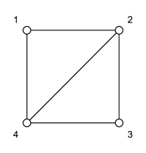
Figure 1:

Remark 2

The inequality ${\rm rk_{H}}(G)\leq\omega(G)$ can be strict for some perfect graphs. This is the case, for instance, for the graph $G$ from Example 1, which is perfect with $\omega(G)=t+1$ and ${\rm rk_{H}}(G)=2$. Figure 1 shows this graph for the case $t=2$.

3.3.2 Odd circuits and their complements

Park and Hong PH12 show that the Handelman rank of an odd circuit is equal to 3. Here we show that the Handelman rank of a weighted odd circuit is at most 3, answering an open question of PH12 , and we also consider the Handelman rank of complements of odd circuits.

Proposition 6

Consider a weighted odd circuit $(C_{2n+1},w)$ and its complement $(\overline{C_{2n+1}},w)$, where the edge weights satisfy (12). Then,

$${\rm rk_{H}}(C_{2n+1},w)\leq 3\ \text{ and }\ {\rm rk_{H}}(\overline{C_{2n+1}},w)\leq n+1.$$

Moreover, equality holds in the unweighted case: ${\rm rk_{H}}(C_{2n+1})=3$ and ${\rm rk_{H}}(\overline{C_{2n+1}})=n+1$.

Proof

For any node $i$, both graphs $C_{2n+1}-i$ and ${C_{2n+1}}\ominus i$ are bipartite and thus ${\rm rk_{H}}(C_{2n+1}-i,w),$ ${\rm rk_{H}}(C_{2n+1}\ominus i,w)\leq 2$ by Corollary 3. Applying Lemma 9, we obtain that ${\rm rk_{H}}(C_{2n+1},w)\leq 3$. Similarly, for any node $i$, both graphs $\overline{C_{2n+1}}-i$ and $\overline{C_{2n+1}}\ominus i$ are perfect with clique number at most $n$ and thus, from Proposition 5, ${\rm rk_{H}}(\overline{C_{2n+1}}-i,w)$, ${\rm rk_{H}}(\overline{C_{2n+1}}\ominus i,w)\leq n$. Applying again Lemma 9 we deduce that ${\rm rk_{H}}(\overline{C_{2n+1}},w)\leq n+1$. In the unweighted case, the lower bounds ${\rm rk_{H}}(C_{2n+1})\geq 3$ and ${\rm rk_{H}}(\overline{C_{2n+1}})\geq n+1$ follow from Proposition 4. Indeed, ${\rm rk_{H}}(C_{2n+1})\geq{2n+1\over\alpha(C_{2n+1})}={2n+1\over n}>2$ and ${\rm rk_{H}}(\overline{C_{2n+1}})\geq{2n+1\over\alpha(\overline{C_{2n+1}})}={2n+1\over 2}>n$. ∎

As an application we obtain the following characterization of perfect graphs, which is in the same spirit as the following well-known characterization due to Lovász Lov72 : $G$ is perfect if and only if $|V(H)|\leq\alpha(H)\omega(H)$ for all induced subgraphs $H$ of $G$.

Corollary 5

A graph $G$ is perfect if and only if ${\rm rk_{H}}(H)\leq\omega(H)$ for every induced subgraph $H$ of $G$.

Proof

The ‘only if’ part follows from Proposition 5. Conversely, assume that $G$ is not perfect. Using the perfect graph theorem of Chudnovsky, Robertson, Seymour and Thomas CRST06 , we know that $G$ contains an induced subgraph $H$ which is an odd circuit or its complement. By Proposition 6, ${\rm rk_{H}}(H)=\chi(H)>\omega(H)$, concluding the proof. ∎

Remark 3

As noted earlier, the upper bound 3 for the Handelman rank of an odd circuit also follows from the upper bound from Corollary 4 in terms of the defect. Indeed, $\alpha^{*}(C_{2n+1})=(2n+1)/2$, so that the defect of the inequality $\sum_{i\in V(C_{2n+1})}x_{i}\leq n=\alpha(C_{2n+1})$ is equal to $2((2n+1)/2-n)=1$ and thus relation (30) gives the upper bound 3.

Park and Hong PH12 show that the Handelman rank of an odd circuit is at most 3 by constructing an explicit decomposition of the polynomial $\alpha(C_{2n+1})-p_{C_{2n+1}}$ in the Handelman set $H_{3}$. We illustrate their argument for the case of $C_{5}$, see Figure 2. Then, we have:

$$\alpha(C_{5})-p_{C_{5}}=2-\sum_{i=1}^{5}x_{i}+\sum_{i=1}^{4}x_{i}x_{i+1}+x_{1}x_{5}=f_{123}+f_{145}+f^{\prime}_{1,34},$$

where

$$f_{123}=1-(x_{1}+x_{2}+x_{3})+x_{1}x_{2}+x_{1}x_{3}+x_{2}x_{3}=(1-x_{1})(1-x_{2})(1-x_{3})+x_{1}x_{2}x_{3}\in H_{3},$$

$$f_{145}=1-(x_{1}+x_{4}+x_{5})+x_{1}x_{4}+x_{1}x_{5}+x_{4}x_{5}=(1-x_{1})(1-x_{4})(1-x_{5})+x_{1}x_{4}x_{5}\in H_{3},$$

$$f^{\prime}_{1,34}=f_{134}(1-x_{1},x_{2},x_{3})=x_{1}-x_{1}x_{3}-x_{1}x_{4}+x_{3}x_{4}=x_{1}(1-x_{3})(1-x_{4})+(1-x_{1})x_{3}x_{4}\in H_{3}.$$

In the above decomposition, $f_{123}$ and $f_{145}$ are the polynomials corresponding to the two cliques $\{1,2,3\}$ and $\{1,4,5\}$ (obtained by adding the edges 13 and 14 to $C_{5}$), and the polynomial $f^{\prime}_{1,34}$ permits to cancel the quadratic terms $x_{1}x_{3}$ and $x_{1}x_{4}$ corresponding to the added edges 13 and 14 and to add the quadratic term $x_{3}x_{4}$. This construction extends easily to an arbitrary odd circuit, showing ${\rm rk_{H}}(C_{2n+1})\leq 3$.

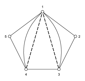
Figure 2: Odd circuit $C_{5}$

We conclude with bounding the Handelman rank of two more classes of graphs.

Example 2

Consider the odd wheel $W_{2n+1}$, which is the graph obtained from an odd circuit $C_{2n+1}$ by adding a new node (the apex node, denoted as $v_{0}$) and making it adjacent to all nodes of $C_{2n+1}$. Since by deleting the apex node $v_{0}$ one obtains $C_{2n+1}$ with Handelman rank 3, Lemma 9 implies that the Handelman rank of the wheel $W_{2n+1}$ is at most 4; note that this bound also holds for any weighted wheel. Moreover, the complement of $W_{2n+1}$ has the same Handelman rank as the complement of $C_{2n+1}$ (since node $v_{0}$ is isolated, and apply Lemma 12 (iv) below).

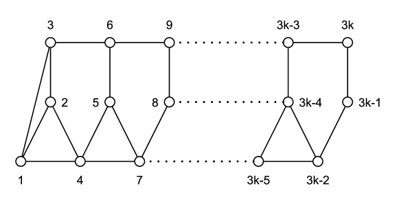
Figure 3: Graph $G_{k}$

Example 3

We now consider the graphs $G_{k}$, constructed by Lipták and Tuncel LT03 and defined as in Figure 3. Hence, for $k=2$, $G_{2}$ is the circuit $C_{5}$ with a new node adjacent to three consecutive nodes of $C_{5}$. We show that, for any $k\geq 2$, the Handelman rank of the graph $G_{k}$ is equal to $3$ or $4$.

As $G_{k}$ has $3k$ nodes and $\alpha(G_{k})=k$, the lower bound (26) for the Handelman rank gives ${\rm rk_{H}}(G_{k})\geq 3$. Now, we look at the upper bound for the Handelman rank. First, we consider the case $k=2$. As in Remark 3, we can give an explicit decomposition for the polynomial $\alpha(G_{2})-p_{G_{2}}$, obtained by adding the chords $(3,4)$ and $(4,6)$ to $G_{2}$. Namely,

$$\alpha(G_{2})-p_{G_{2}}=f_{1234}+f_{456}+f^{\prime}_{4,36},$$

where

$$f_{1234}=1-\sum_{i=1}^{4}x_{i}+\sum_{1\leq i<j\leq 4}x_{i}x_{j}\in H_{4},$$

$$f_{456}=1-\sum_{i=4}^{6}x_{i}+(x_{4}x_{5}+x_{4}x_{6}+x_{5}x_{6})\in H_{3},$$

$$f^{\prime}_{4,36}=f_{436}(1-x_{4},x_{3},x_{6})=x_{4}(1-x_{3})(1-x_{6})+(1-x_{4})x_{3}x_{6}\in H_{3}.$$

In the above decomposition, $f_{1234}$ and $f_{456}$ are the polynomials corresponding to the two cliques $\{1,2,3,4\}$ and $\{4,5,6\}$ (obtained by adding the edges $34$ and $46$ to $G_{2}$), and the polynomial $f^{\prime}_{4,36}$ permits to cancel the quadratic terms $x_{3}x_{4}$ and $x_{4}x_{6}$ corresponding to the added edges $34$ and $46$ and to add the quadratic term $x_{3}x_{6}$.

This construction extends easily to an arbitrary $k\geq 3$, showing ${\rm rk_{H}}(G_{k})\leq 4$. For example, $\alpha(G_{3})-p_{G_{3}}=f_{1234}+f_{4567}+f_{789}+f^{\prime}_{4,36}+f^{\prime}_{7,69}\in H_{4}$.

Observe that the upper bound from Corollary 4 is not strong enough to show this. Indeed the defect of the inequality $\sum_{i\in V(G_{k})}x_{i}\leq\alpha(G_{k})=k$ is equal to $2(\alpha^{*}(G_{k})-\alpha(G_{k}))=k$, since $\alpha(G_{k})=k$ and $\alpha^{*}(G_{k})=3k/2$ (this follows from the fact $\sum_{i\in V(G_{k})}x_{i}\leq\alpha(G_{k})$ defines a facet of $\text{\rm ST}(G_{k})$, shown in (LT03, , Lemma 32 and Theorem 34), so that $\alpha^{*}(G_{k})=3k/2$ by Lemma 2.10 of LS91 ). Thus Corollary 4 permits only to conclude that ${\rm rk_{H}}(G_{k})\leq k+2$.

3.4 Graph operations

In this subsection, we investigate the behavior of the Handelman rank under some graph operations like node or edge deletion, edge contraction, and taking clique sums. For simplicity, we only consider unweighted graphs, while some of the results can easily be extended to the weighted case.

3.4.1 Operations on edges and nodes

An interesting observation is that the Handelman rank is not monotone under edge deletion. As an illustration, look at the three graphs in Figure 4. Consider the first complete graph $K_{4}$ with ${\rm rk_{H}}(K_{4})=4$. If we delete one edge (say edge 13), we obtain the second graph $G$ with rank ${\rm rk_{H}}(G)=2$. However, if we additionally delete the edges 12 and 14, then the third graph $G^{\prime}=K_{4}\setminus\{12,13,14\}$ has ${\rm rk_{H}}(G^{\prime})=3$, since it is the clique 0-sum of a node and a clique of size 3. (See Lemma 13 below.) On the other hand, if we delete an edge whose deletion increases the stability number (a so-called critical edge), then the Handelman rank does not increase.

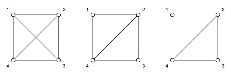
Figure 4:

Lemma 11

Let $e$ be an edge of $G$ such that $\alpha(G\setminus e)=\alpha(G)+1$. Then, ${\rm rk_{H}}(G\setminus e)\leq{\rm rk_{H}}(G)$.

Proof

Say $e$ is the edge 12. Then, $\alpha(G\setminus e)-p_{G\setminus e}=\alpha(G)-p_{G}+1-x_{1}x_{2}.$ As $1-x_{1}x_{2}=1-x_{2}+x_{2}(1-x_{1})\in H_{2}$, this implies that ${\rm rk_{H}}(G\setminus e)\leq{\rm rk_{H}}(G)$. ∎

The Handelman rank is not monotone under edge contraction either. For instance, the graph $G$ in Figure 1 has ${\rm rk_{H}}(G)=2$. If we contract the edge 23, we get the new graph $G^{\prime}$ is a triangle with ${\rm rk_{H}}(G^{\prime})=3$. If we contract one more edge 12, the resulting graph $G^{\prime\prime}$ is an edge with ${\rm rk_{H}}(G^{\prime\prime})=2$. Analogously, deleting a node can either increase, decrease or not affect the Handelman rank. We group several properties about the behavior of the Handelman rank under node deletion.

Lemma 12

Let $G=(V,E)$ be a graph and $j\in V$.

• If $\alpha(G-j)=\alpha(G)$, then ${\rm rk_{H}}(G-j)\leq{\rm rk_{H}}(G).$

• If $\alpha(G-j)=\alpha(G)-1$, then ${\rm rk_{H}}(G)\leq{\rm rk_{H}}(G-j)$.

• If $j$ is adjacent to all other nodes of $G$, then ${\rm rk_{H}}(G)\leq{\rm rk_{H}}(G-j)+1$.

• If $j$ is an isolated node, then ${\rm rk_{H}}(G)={\rm rk_{H}}(G-j)$.

Proof

(i) We use relation (28) applied to the polynomial $f_{G}$ (and node $j$). As before $\underline{x}$ consists of all variables except $x_{j}$, so that $x=(\underline{x},x_{j})$. As $\alpha(G-j)=\alpha(G)$, we have $f_{G-j}(\underline{x})=f_{G}(\underline{x},0)\in H_{{\rm rk_{H}}(G)}$, which implies ${\rm rk_{H}}(G-j)\leq{\rm rk_{H}}(G)$.

(ii) If $\alpha(G-j)=\alpha(G)-1$, then $f_{G}=f_{G-j}+(1-x_{j})+\sum_{i:ij\in E}w_{ij}x_{i}x_{j}\in H_{{\rm rk_{H}}(G-j)}$. Hence, ${\rm rk_{H}}(G)\leq{\rm rk_{H}}(G-j)$.

(iii) Assume that $j$ is adjacent to all other nodes of $G$. If $G-j$ has no edge then $G$ is bipartite and thus ${\rm rk_{H}}(G)=2={\rm rk_{H}}(G-j)+1$. Assume now that $G-j$ has an edge so that ${\rm rk_{H}}(G-j)\geq 2$. Using Lemma 9, we deduce that ${\rm rk_{H}}(G)\leq{\rm rk_{H}}(G-j)+1$.

(iv) $G$ is the clique 0-sum of $G-j$ and the single node $j$, and we can apply Lemma 13 below. ∎

Remark 4

In Lemma 12 (ii), the gap ${\rm rk_{H}}(G-j)-{\rm rk_{H}}(G)$ can be arbitrarily large. To see this consider the graph $G$ obtained by taking the clique $t$-sum of $K_{2t}$ and $K_{t+1}$ along a common $K_{t}$. Let $j$ be the node of $K_{t+1}$ which does not belong to the common clique $K_{t}$. If we delete node $j$, then $G-j=K_{2t}$ has ${\rm rk_{H}}(G-j)=2t$. On the other hand, ${\rm rk_{H}}(G)\leq t+1$, since $\alpha(G)=2=\rho_{t+1}(G)$ as $V(G)$ can be covered by two cliques of size at most $t+1$. Thus ${\rm rk_{H}}(G-j)-{\rm rk_{H}}(G)\geq 2t-(t+1)=t-1$.

3.4.2 Clique sums

Suppose $G=(V,E)$ is the clique $t$-sum of two graphs $G_{1}$ and $G_{2}$. We now study the Handelman rank of $G$, whose value needs technical case checking, depending on the values of the stability numbers of $G$, $G_{1}$, $G_{2}$ and of some subgraphs.

Lemma 13

Suppose $G$ is the clique $t$-sum of $G_{1}$ and $G_{2}$ along a common $t$-clique $C_{0}$ and let $H_{i}=G_{i}\setminus C_{0}$ for $i=1,2$. The following holds.

• If $\alpha(G)=\alpha(G_{1})+\alpha(G_{2})$, then

  $${\rm rk_{H}}(G)\leq\min\{\max\{{\rm rk_{H}}(G_{1}),{\rm rk_{H}}(H_{2})\},\max\{{\rm rk_{H}}(H_{1}),{\rm rk_{H}}(G_{2}))\}\}.$$

  Moreover, ${\rm rk_{H}}(G)\leq\max\{{\rm rk_{H}}(G_{1}),{\rm rk_{H}}(G_{2})\}$ if $t\leq 3$.

• Assume $\alpha(G)=\alpha(G_{1})+\alpha(G_{2})-1$. Then $\alpha(G_{k})=\alpha(H_{k})+1$ for (say) $k=1$ and ${\rm rk_{H}}(G)\leq\max\{{\rm rk_{H}}(H_{1}),{\rm rk_{H}}(G_{2})\}$.

• Assume $\alpha(G)=\alpha(G_{1})+\alpha(G_{2})-2$. For $k\in\{1,2\}$ let $C_{k}$ denote the set of nodes of $C_{0}$ which belong to at least one maximum stable set of $G_{k}$. Set $H^{\prime}_{1}=G_{1}\backslash C_{1}$ and $H^{\prime}_{2}=G\setminus H_{1}^{\prime}=G_{2}\setminus(C_{0}\setminus C_{1})$. Then $\alpha(H^{\prime}_{k})=\alpha(G_{k})-1$ for $k=1,2$, and ${\rm rk_{H}}(G)\leq\max\{{\rm rk_{H}}(H^{\prime}_{1}),{\rm rk_{H}}(H^{\prime}_{2})\}$.

Proof

In what follows, for subsets $A,B\subseteq V$, $E(A,B)$ denotes the set of edges $ij$ with $i\in A$ and $j\in B$, and $E(A)$ the set of edges contained in $A$. We also set $VG$ for $V(G)$.
(i) We use the identities

$$f_{G}=f_{G_{1}}+f_{H_{2}}+(\alpha(G)-\alpha(G_{1})-\alpha(H_{2}))+\sum_{ij\in E(VG_{1},VH_{2})}x_{i}x_{j},$$

$$f_{G}=f_{G_{2}}+f_{H_{1}}+(\alpha(G)-\alpha(G_{2})-\alpha(H_{1}))+\sum_{ij\in E(VG_{2},VH_{1})}x_{i}x_{j}.$$

As $\alpha(G)=\alpha(G_{1})+\alpha(G_{2})$, $\alpha(G)-\alpha(G_{1})=\alpha(G_{2})\geq\alpha(H_{2})$ and $\alpha(G)-\alpha(G_{2})=\alpha(G_{1})\geq\alpha(H_{1})$, implying ${\rm rk_{H}}(G)\leq\min\{\max\{{\rm rk_{H}}{(G_{1})},{\rm rk_{H}}(H_{2})\},\max\{{\rm rk_{H}}{(G_{2})},{\rm rk_{H}}{(H_{1})}\}\}.$ For the second statement, we use the identity

$$f_{G}=f_{G_{1}}+f_{G_{2}}+\sum_{i\in C_{0}}x_{i}-\sum_{ij\in E(C_{0})}x_{i}x_{j}$$

combined with the fact that $\sum_{i\in C_{0}}x_{i}-\sum_{ij\in E(C_{0})}x_{i}x_{j}\in H_{2}$ when $t=|C_{0}|\leq 3$. This is clear if $t\leq 1$ and follows from the identities $x_{1}+x_{2}-x_{1}x_{2}=x_{1}(1-x_{2})+x_{2}\in H_{2}$ and $x_{1}+x_{2}+x_{3}-x_{1}x_{2}-x_{1}x_{3}-x_{2}x_{3}=x_{1}(1-x_{2})+x_{2}(1-x_{3})+x_{3}(1-x_{1})\in H_{2}$ if $t=2,3$. From this follows that ${\rm rk_{H}}(G)\leq\max\{{\rm rk_{H}}(G_{1}),{\rm rk_{H}}(G_{2})\}$.

(ii) As $\alpha(G)\neq\alpha(G_{1})+\alpha(G_{2})$, it follows that $\alpha(H_{k})=\alpha(G_{k})-1$ for at least one index $k=1,2$. Say this holds for $k=1$. Then we use the identities

$$f_{G}=f_{G_{1}}+f_{G_{2}}-1+\sum_{i\in C_{0}}x_{i}-\sum_{ij\in E(C_{0})}x_{i}x_{j},$$

and

$$f_{H_{1}}=f_{G_{1}}-1+\sum_{i\in C_{0}}x_{i}-\sum_{ij\in E(C_{0})}x_{i}x_{j}-\sum_{ij\in E(C_{0},VG_{1}\setminus C_{0})}x_{i}x_{j}.$$

This gives:

$$f_{G}=f_{H_{1}}+f_{G_{2}}+\sum_{ij\in E(C_{0},VG_{1}\setminus C_{0})}x_{i}x_{j},$$

which implies ${\rm rk_{H}}(G)\leq\max\{{\rm rk_{H}}(H_{1}),{\rm rk_{H}}(G_{2})\}.$

(iii) By construction, $\alpha(H_{1}^{\prime})=\alpha(G_{1})-1$. Moreover, as $\alpha(G)=\alpha(G_{1})+\alpha(G_{2})-2$, it follows that $C_{1}\cap C_{2}=\emptyset$ and thus $\alpha(H^{\prime}_{2})=\alpha(G_{2})-1$. We now use the identities

$$f_{H^{\prime}_{1}}=f_{G_{1}}-1+\sum_{i\in C_{1}}x_{i}-\sum_{ij\in E(C_{1})\cup E(C_{1},VG_{1}\setminus C_{1})}x_{i}x_{j},$$

$$f_{H^{\prime}_{2}}=f_{G_{2}}-1+\sum_{i\in C_{0}\setminus C_{1}}x_{i}-\sum_{ij\in E(C_{0}\setminus C_{1})\cup E(C_{0}\setminus C_{1},VG_{2}\setminus(C_{0}\setminus C_{1}))}x_{i}x_{j},$$

and

$$f_{G}=f_{G_{1}}+f_{G_{2}}-2+\sum_{i\in C_{0}}x_{i}-\sum_{ij\in E(C_{0})}x_{i}x_{j}.$$

Combining these relations, we obtain

$$f_{G}=f_{H^{\prime}_{1}}+f_{H^{\prime}_{2}}+\sum_{ij\in E(C_{1},VG_{1}\setminus C_{1})\cup E(C_{0}\setminus C_{1},VG_{2}\setminus C_{0})}x_{i}x_{j}$$

which shows ${\rm rk_{H}}(G)\leq\max\{{\rm rk_{H}}(H_{1}^{\prime}),{\rm rk_{H}}(H_{2}^{\prime})\}$. ∎

In the special case when $G$ is a clique sum of two cliques, one can easily determine the the exact value of the Handelman rank of $G$.

Lemma 14

Assume that $G$ is the clique $t$-sum of two cliques $K_{n_{1}}$ and $K_{n_{2}}$ with $n_{1}\leq n_{2}$. Then, ${\rm rk_{H}}(G)=\max\{\lceil\frac{n_{1}+n_{2}-t}{2}\rceil,n_{2}-t\}$.

Proof

Obviously, $\alpha(G)=2$. Define $n=|V(G)|=n_{1}+n_{2}-t$. Assume first that $n_{2}-n_{1}\leq t$. Then $V(G)$ can be covered by two cliques of sizes $\lceil\frac{n}{2}\rceil$ and $\lfloor\frac{n}{2}\rfloor$ and thus ${\rm rk_{H}}(G)\leq\lceil\frac{n}{2}\rceil$. In addition, by (26), ${\rm rk_{H}}(G)\geq{n\over\alpha(G)}={n\over 2}$. Hence we obtain ${\rm rk_{H}}(G)=\lceil\frac{n}{2}\rceil=\max\{\lceil\frac{n}{2}\rceil,n_{2}-t\}$.

Assume now that $n_{2}-n_{1}>t$. Then $G$ can be covered by two cliques of sizes $n_{1}$ and $n_{2}-t$, which implies ${\rm rk_{H}}(G)\leq n_{2}-t$. On the other hand, by applying Lemma 12 (i) to all nodes $i$ in the common $t$-clique, together with Lemma 13, we obtain the reverse inequality ${\rm rk_{H}}(G)\geq\max\{{\rm rk_{H}}(K_{n_{2}-t}),{\rm rk_{H}}(K_{n_{1}-t})\}=n_{2}-t$. ∎

4 Links to other hierarchies

Several other hierarchies have been considered in the literature for general 0/1 optimization problems applying also to the maximum stable set problem, in particular, by Sherali and Adams SA90 , by Lovász and Schrijver LS91 , by Lasserre Las02 , and by de Klerk and Pasechnik KP02 . We briefly indicate how they relate to the Handelman hierarchy considered in this paper, based on optimization on the hypercube.

4.1 Sherali-Adams and Lasserre hierarchies

Consider the following $0-1$ polynomial optimization problem:

$$\max\ \ p(x)\ \ {\rm{s.t.}}\ \ x\in K\cap\{0,1\}^{n},$$ (31)

which is obtained by adding the integrality constraint $x\in\{0,1\}^{n}$ to problem (1). Recall that ${\mathcal{I}}$ denotes the ideal generated by $x_{i}-x_{i}^{2}$ for $i\in[n]$ and that the Handelman set $H_{t}$ is defined in (6). Sherali and Adams SA90 introduce the following bounds for (31):

$$p_{\text{sa}}^{(t)}=\inf\left\{\lambda:\lambda-p\in H_{t}+\sum_{j=1}^{m}g_{j}H_{t-\deg(g_{j})}+{\mathcal{I}}\right\}.$$ (32)

The above program is in fact the dual of the linear program usually used to define the Sherali-Adams bounds. For details we refer e.g. to SA90 ; Las02b ; Lau03 .

When applying the Sherali-Adams construction to the maximum stable set problem for the instance $(G,w)$, the starting point is to formulate $\alpha(G,w)$ as the problem of maximizing the linear polynomial $p(x)=w^{T}x=\sum_{i\in[n]}w_{i}x_{i}$ over $K\cap\{0,1\}^{n}$, where $K=\text{\rm FR}(G)$ is the fractional stable set polytope, so that the corresponding bound from (32) reads

$$p_{\text{\rm sa}}^{(t)}(G,w)=\inf\left\{\lambda:\lambda-w^{T}x\in H_{t}+\sum_{ij\in E}(1-x_{i}-x_{j})H_{t-1}+{\mathcal{I}}\right\}.$$ (33)

For $t\geq 2$, let $\langle x_{i}x_{j}:ij\in E\rangle_{t}$ denote the truncated ideal consisting of all polynomials $\sum_{ij\in E}u_{ij}x_{i}x_{j}$ where $u_{ij}\in{\mathbb{R}}[x]$ has degree at most $t-2$. One can formulate the following variation of the bound (33):

$$\text{\rm sa}^{(t)}(G,w)=\min\{\lambda:\lambda-w^{T}x\in H_{t}+\langle x_{i}x_{j}:ij\in E\rangle_{t}+{\mathcal{I}}\},$$

which satisfies $\text{\rm sa}^{(t+1)}(G,w)\leq p_{\text{\rm sa}}^{(t)}(G,w)\leq\text{\rm sa}^{(t)}(G,w).$ (To see it use, for any edge $ij\in E$, the identities $1-x_{i}-x_{j}=(1-x_{i})(1-x_{j})-x_{i}x_{j}$ and $-x_{i}x_{j}=x_{i}(1-x_{i}-x_{j})+x_{i}(x_{i}-1)$.) Comparing with the hypercube based Handelman bound (15), we see that

$$\text{\rm sa}^{(t)}(G,w)\leq p_{\text{\rm han}}^{(t)}(G,w),$$

since $\lambda-p_{G,w}=\lambda-w^{T}x+\sum_{ij\in E}w_{ij}x_{i}x_{j}\in H_{t}$ implies $\lambda-w^{T}x\in H_{t}+\langle x_{i}x_{j}:ij\in E\rangle_{t}$.

We now recall the following semidefinite programming bound of Lasserre Las02 :

$$\text{las}^{(t)}(G,w)=\min\{t:\lambda-w^{T}x\in\Sigma_{2t}+\langle x_{i}x_{j}:ij\in E\rangle_{t}+{\mathcal{I}}\},$$

where $\Sigma_{2t}$ is the set of polynomials of degree at most $2t$ which can be written as a sum of squares of polynomials. As is well known,

$$\text{las}^{(t)}(G,w)\leq\text{\rm sa}^{(t)}(G,w);$$

this can easily be seen by noting that, for any set $T$ with $|T|=t$, we have

$$x^{I}(1-x)^{T\setminus I}=\underbrace{\prod_{i\in I}x_{i}^{2}\prod_{j\in T\setminus I}(1-x_{j})^{2}}_{\in\Sigma_{2t}}+\underbrace{\left(\prod_{i\in I}x_{i}\prod_{j\in T\setminus I}(1-x_{j})-\prod_{i\in I}x_{i}^{2}\prod_{j\in T\setminus I}(1-x_{j})^{2}\right)}_{\in{\mathcal{I}}},$$

where the second term belongs to ${\mathcal{I}}$ in view of Lemma 3. Summarizing, we have

$$\alpha(G,w)\leq\text{las}^{(t)}(G,w)\leq\text{\rm sa}^{(t)}(G,w)\leq p_{\text{\rm han}}^{(t)}(G,w).$$

Hence, the Sherali-Adams and Lasserre bounds are at least as strong as the Handelman bound at any given order $t$, however they are more expensive to compute. Indeed the Sherali-Adams bound is linear but its definition involves more terms, and the Lasserre bound is based on semidefinite programming which is computationally more demanding than linear programming. For more results about the comparison between Sherali-Adams and Lasserre hierarchies, see e.g. Las02b ; Lau03 .

4.2 Lovász-Schrijver hierarchy

Given a polytope $K\subseteq[0,1]^{n}$, Lovász and Schrijver LS91 build a hierarchy of polytopes nested between $K$ and the convex hull of $K\cap\{0,1\}^{n}$ that finds it after $n$ steps. When applied to the maximum stable set problem, one starts with the fractional stable set polytope $K=\text{\rm FR}(G)$. For convenience set ${\widehat{V}}=V\cup\{0\}$ (where $0$ is an additional element not belonging to $V$) and define the cone

$${\mathcal{C}}(G)=\left\{\lambda{1\choose x}:x\in\text{\rm FR}(G),\lambda\geq 0\right\}\subseteq{\mathbb{R}}^{{\widehat{V}}}.$$

Define the following set of symmetric matrices indexed by ${\widehat{V}}$:

$${\mathcal{M}}(G)=\{Y\in{\mathcal{S}}_{\widehat{V}}:Y_{ii}=Y_{0i}\ \forall i\in V,\ Ye_{i},Y(e_{0}-e_{i})\in{\mathcal{C}}(G)\ \forall i\in V\}$$

and the corresponding subset of ${\mathbb{R}}^{V}$:

$$N(\text{\rm FR}(G))=\left\{x\in{\mathbb{R}}^{V}:{1\choose x}=Ye_{0}\ \ {\text{for some}}\ \ Y\in{\mathcal{M}}(G)\right\}.$$

For $t\geq 2$, define the $t$-th iterate $N^{t}(\text{\rm FR}(G))=N(N^{t-1}(\text{\rm FR}(G)))$, setting $N^{1}(\text{\rm FR}(G))=N(\text{\rm FR}(G))$. It is shown in LS91 that

$$\text{\rm ST}(G)\subseteq\ldots\subseteq N^{t}(\text{\rm FR}(G))\subseteq N^{t-1}(\text{\rm FR}(G))\subseteq\ldots\subseteq N(\text{\rm FR}(G))\subseteq\text{\rm FR}(G),$$

with equality $\text{\rm ST}(G)=N^{n}(\text{\rm FR}(G))$. By maximizing the linear function $w^{T}x$ over $N^{t}(\text{\rm FR}(G))$ we get the bound $\text{ls}^{(t)}(G,w)$ which satisfies $p_{\text{\rm sa}}^{(t+1)}(G,w)\leq\text{ls}^{(t)}(G,w)$ for $t\geq 1$ (see LS91 ; Lau03 ).

For any $w\in{\mathbb{R}}^{V}_{+}$, the corresponding inequality $w^{T}x\leq\alpha(G,w)$ is valid for $\text{\rm ST}(G)$. Following LS91 , its $N$-index, denoted as $\text{rk}_{\text{LS}}(G,w)$, is the smallest integer $t$ for which the inequality $w^{T}x\leq\alpha(G,w)$ is valid for $N^{t}(\text{\rm FR}(G))$ or, equivalently, $\alpha(G,w)=\text{ls}^{(t)}(G,w)$. The following bounds are shown in LS91 for the $N$-index:

$${\sum_{i=1}^{n}w_{i}\over\alpha(G,w)}-2\leq\text{rk}_{\text{LS}}(G,w)\leq\text{\rm defect}(G,w),\ \text{rk}_{\text{LS}}(G,w)\leq|V(G)|-\alpha(G)-1,$$

where $\text{\rm defect}(G,w)$ is as defined in (29). Note the analogy with the bounds (26), (27) and (30) for the Handelman rank. There is a shift of 2 between the two hierarchies which can be explained from the fact that the Lovász-Schrijver construction starts from the fractional stable set polytope which already takes the edges into account, so that $\text{ls}^{(0)}(G,w)=\alpha^{*}(G,w)=p_{\text{\rm han}}^{(2)}(G,w)$. We also observe this shift by 2, e.g., in the results for perfect graphs and for odd cycles and wheels. It seems moreover that the Handelman bound and the bound obtained by using the $N$-operator are closely related. We did some computational tests for the graphs $K_{4}$, $W_{5}$ and $G_{k}$ ($k=2,3,4,5$) with different weight functions; in all cases we observe that both bounds coincide, i.e., $\text{ls}^{(1)}(G,w)=p_{\text{\rm han}}^{(3)}(G,w)$ holds. Understanding the exact link between the two hierarchies of Handelman and of Lovász-Schrijver is an interesting open question.

4.3 De Klerk and Pasechnik LP hierarchy

Given a graph $G=(V,E)$ with adjacency matrix $A$, de Klerk and Pasechnik KP02 formulate its stability number via the following copositive program:

$$\alpha(G)=\min\{\lambda:\lambda(I+A)-ee^{T}\in{\mathcal{C}}_{n}\},$$

which is based on the Motzkin-Straus formulation:

$${1\over\alpha(G)}=\min_{x\in\Delta}x^{T}(I+A)x,$$ (34)

where $\Delta=\{x\in{\mathbb{R}}^{V}_{+}:\sum_{i=1}^{n}x_{i}=1\}$ is the standard simplex. As problem (34) is the problem of minimizing the quadratic polynomial $q(x)=x^{T}(I+A)x$ over the simplex $\Delta$, one can follow the approach sketched in Section 1.2 and define, for any $t\geq 2$, the corresponding (simplex based) Handelman bound

$$q_{\text{han}}^{(t)}=\max\{\lambda:(q-\lambda\sigma^{2})\sigma^{t-2}\in{\mathbb{R}}_{+}[x]\},$$

where $\sigma=\sum_{i=1}^{n}x_{i}$. (Recall Lemma 1.) It turns out that it can be computed explicitly since it is directly related to the following bound introduced in KP02 :

$$\zeta^{(t)}(G)=\min\{\mu:(\mu q-\sigma^{2})\sigma^{t}\in{\mathbb{R}}_{+}[x]\}$$

for any $t\geq 0$. Indeed it follows from the definitions that

$$\zeta^{(t)}q_{\text{han}}^{(t+2)}=1\ \text{ for }t\geq 0.$$

De Klerk and Pasechnik KP02 show that

$$\zeta^{(0)}(G)\geq\zeta^{(1)}(G)\geq\cdots\geq\lfloor\zeta^{(t)}(G)\rfloor=\alpha(G)$$

for $t\geq\alpha(G)^{2}{-1}$. Moreover, Peña, Vera and Zuluaga PVZ12 give the following closed-form expression for the parameter $\zeta^{(t)}(G)$:

$$\zeta^{(t)}(G)=\frac{{t+2\choose 2}}{{u\choose 2}\alpha(G)+uv},\ \ \text{ where }t+2=u\alpha(G)+v\text{ with }u,v\in{\mathbb{N}}\text{ and }v<\alpha(G).$$

From this we see that $\zeta^{(t)}(G)=\infty$ if $t\leq\alpha(G)-2$ and $\zeta^{(t)}(G)=\alpha(G)+1$ if $t=\alpha(G)^{2}-2$. Moreover, $\alpha(G)\leq\zeta^{(t)}(G)<\alpha(G)+1$ for any $t\geq\alpha(G)^{2}-1$, with a strict inequality $\alpha(G)<\zeta^{(t)}(G)$ if $G$ is not a complete graph. Hence, in contrast to the LP bounds based on the Handelman, Sherali-Adams and Lovász-Schrijver constructions (which are exact at order $n$), the LP copositive-based bound is never exact (except for the complete graph), one needs to round it in order to obtain the stability number.

From the above discussion it follows that the LP copositive rank ${\rm{rk}}_{\text{KP}}(G)$, which we define as the smallest integer $t$ such that $\lfloor\zeta^{(t)}(G)\rfloor=\alpha(G)$, can be determined exactly: ${\rm{rk}}_{\rm KP}(G)=\alpha(G)^{2}-1$ for any graph $G$. We now observe that it cannot be compared with the (hypercube based) Handelman rank ${\rm rk_{H}}(G)$. Indeed, for the complete graph $G=K_{n}$, we have ${\rm{rk}}_{\text{KP}}(K_{n})=0$ while ${\rm rk_{H}}(K_{n})=n$. On the other hand, the graph $K_{1,n}$ has ${\rm{rk}}_{\text{KP}}(K_{1,n})=n^{2}-1$ and ${\rm rk_{H}}(K_{1,n})=2$. As another example, for the graph $G_{k}$ from Example 3, ${\rm{rk}}_{\text{KP}}(G_{k})=k^{2}-1$ while ${\rm rk_{H}}(G_{k})\leq 4$. Hence the ranks of the two hierarchies are not comparable. These examples also show that the ranks of the Lovász-Schrijver and of the LP copositive hierarchies are not comparable, since ${\rm{rk}}_{\rm LS}(K_{n})=n-2$ and ${\rm{rk}}_{\rm LS}(K_{1,n})=0$.

5 The Handelman hierarchy for the maximum cut problem

In this paper we have studied how the (hypercube based) Handelman hierarchy applies to the maximum stable set problem. A main motivation for studying this hierarchy is that, due to its simplicity, it is easier to analyze than other hierarchies. We proved several properties that seem to indicate that there is a close relationship to the hierarchy of Lovász-Schrijver, whose exact nature still needs to be investigated. Another interesting open question is whether the Handelman rank is upper bounded in terms the tree-width of the graph.

We now conclude with some observations clarifying how the Handelman hierarchy applies to the maximum cut problem. Given a graph $G=(V,E)$ with edge weights $w\in{\mathbb{R}}^{E}$, the max-cut problem asks to find a partition $(V_{1},V_{2})$ of the node set $V$ so that the total weight of the edges cut by the partition is maximized; it is NP-hard, already in the unweighted case Karp72 . As observed in PH11 the formulation (3) extends to the weighted case:

$${\rm mc}(G,w)=\max_{x\in[0,1]^{n}}\sum_{i\in V}d_{i}x_{i}-2\sum_{ij\in E}w_{ij}x_{i}x_{j},$$

setting $d_{i}=\sum_{j\in V:ij\in E}w_{ij}.$ As the polynomial $p(x)=\sum_{i\in V}d_{i}x_{i}-2\sum_{ij\in E}w_{ij}x_{i}x_{j}$ is square-free the Handelman bound of order $t$ can be formulated as

$$\min\{\lambda:\lambda-p\in H_{t}\}.$$

We show below that it can be equivalently reformulated in a more explicit way in terms of suitable valid inequalities for the cut polytope. We need some definitions. The cut polytope $\text{CUT}_{n}$ is defined as the convex hull of the vectors $(v_{i}v_{j})_{1\leq i<j\leq n}$ for all $v\in\{\pm 1\}^{n}$. So $\text{\rm CUT}_{n}$ is a polytope in the space ${\mathbb{R}}^{n\choose 2}$ indexed by the edge set of the complete graph $K_{n}$. Given an integer $t\geq 2$, among all the inequalities that are valid for $\text{\rm CUT}_{n}$, we consider only those that are supported by at most $t$ points of $[n]$ and we let $P^{(t)}_{n}$ denote the polytope in ${\mathbb{R}}^{n\choose 2}$ defined by all these selected inequalities. Clearly, $\text{\rm CUT}_{n}\subseteq P^{(t)}_{n}$. Moreover, for $n\neq 4$, equality $\text{\rm CUT}_{n}=P^{(t)}_{n}$ holds if and only if $t=n$ (since $\text{\rm CUT}_{n}$ has some facet defining ineqaulities supported by $n$ points). The case $n=4$ is an exception since $\text{\rm CUT}_{4}=P^{(3)}_{4}$.

Proposition 7

Let $t\geq 2$ and, given an edge weighted graph $(G,w)$, consider the above mentioned polynomial $p=\sum_{i\in V}d_{i}x_{i}-2\sum_{ij\in E}w_{ij}x_{i}x_{j}$. The following equality holds:

$$\min\{\lambda:\lambda-p\in H_{t}\}=\max_{y\in P^{(t)}_{n}}\sum_{ij\in E}w_{ij}(1-y_{ij})/2.$$

Proof

It is convenient to use $\pm 1$ valued variables $z$ instead of the $0/1$ valued variables $x$. So we set $z_{i}=1-2x_{i}$ for $i\in[n]$. Then $p(x)=q(z)$, after defining the polynomial $q(z)=\sum_{ij\in E}w_{ij}(1-z_{i}z_{j})/2$. Moreover define the $\pm 1$ analogue of the Handelman set $H_{t}$ from (6):

$$\overline{H}_{t}=\{\sum_{T\subseteq[n]:|T|=t}\sum_{I\subseteq T}c_{I,T}(1-z)^{I}(1+z)^{T\setminus I}:c_{I,T}\geq 0\}.$$

Furthermore let $\overline{\mathcal{I}}$ denote the ideal in the polynomial ring ${\mathbb{R}}[z]$ generated by $z_{i}^{2}-1$ for $i\in[n]$, and let $\overline{\mathcal{I}}_{t}$ denote its truncation at degree $t$. One can easily verify that $\lambda-p\in H_{t}$ if and only if $\lambda-q\in\overline{H}_{t}$ which, in turn, is equivalent to $\lambda-q\in\overline{H}_{t}+\overline{\mathcal{I}}_{t}$. Therefore we have

$$\min\{\lambda:\lambda-p\in H_{t}\}=\min\{\lambda:\lambda-q\in\overline{H}_{t}+\overline{\mathcal{I}}_{t}\}.$$

Now we apply LP duality and obtain that the last program is equal to

$$\max_{L}\{L(q):L(1)=1,\ L(f)\geq 0\ \forall f\in\overline{H}_{t},\ L(f)=0\ \forall f\in\overline{\mathcal{I}}_{t}\},$$

where the maximum is taken over all linear functionals $L:{\mathbb{R}}[z]_{t}\rightarrow{\mathbb{R}}$. Finally, we use the fact that this maximization program is equal to the maximum of $\sum_{ij\in E}w_{ij}(1-y_{ij})/2$ taken over all $y\in P^{(t)}_{n}$, which is shown in Lau03 (top of page 20). This concludes the proof. ∎

For instance, for $t=2$, $P^{(2)}_{n}=[-1,1]^{n\choose 2}$ (since $-1\leq y_{ij}\leq 1$ are the only inequalities on two points valid for $\text{\rm CUT}_{n}$). Hence, by Proposition 7, the Handelman bound of order 2 is equal to $\sum_{ij\in E}|w_{ij}|$, as shown in PH11 for the case $w\geq 0$. For $t=3$, $P^{(3)}_{n}$ is defined by the triangle inequalities $y_{ij}+y_{ik}+y_{jk}\geq-1$ and $y_{ij}-y_{ik}-y_{jk}\geq-1$ for all $i,j,k\in[n]$. Therefore, for an edge weighted graph $G$ where $G$ has no $K_{5}$ minor, we find that the Handelman bound of order 3 is exact and returns the value of the maximum cut (since the triangle inequalities suffice to describe the cut polytope of $G$, after taking projections). In particular, the Handelman rank is at most 3 for a weighted odd circuit, which answers an open question of PH12 (which shows the result in the unweighted case). As a final observation, we find that the rank of the Handelman hierarchy for the maximum cut problem in $K_{n}$ is equal to $n$ for any $n\neq 4$ (which was shown in PH11 for $n$ odd).

- (1) Bruck, J., Blaum, M.: Neural networks, error-correcting codes, and polynomials over the binary -cube. IEEE transactions on information theory. 35(5), 976-987 (1989)
- (2) Chudnovsky, M., Robertson, N., Seymour, P., Thomas, R.: The strong perfect graph theorem. Ann. Math. 164(1), 51-229 (2006)
- (3) Cornaz, D., Jost, V.: A one-to-one correspondance between colorings and stable sets. Oper. Res. Lett. 36(6), 673-676 (2008)
- (4) Faybusovich, L.: Global optimization of homogeneous polynomials on the simplex and on the sphere. In: Floudas, C., Pardalos, P. (eds.) Frontiers in Global Optimization, pp. 109-121. Kluwer Academic Publishers, Dordrecht (2003)
- (5) De Klerk, E., Laurent, M.: Error bounds for some semidefinite programming approaches to polynomial optimization on the hypercube. SIAM J. Optim. 20(6), 3104-3120 (2010)
- (6) De Klerk, E., Laurent, M., Parrilo, P.: On the equivalence of algebraic approaches to the minimization of forms on the simplex. In: Henrion, D.,Garulli, A. (eds.) Positive Polynomials in Control, pp. 121-133. Springer Verlag, Berlin (2005)
- (7) De Klerk, E., Laurent, M., Parrilo, P.: A PTAS for the minimization of polynomials of fixed degree over the simplex. Theor. Comput. Sci. 361(2-3), 210-225 (2006)
- (8) De Klerk, E., Pasechnik, D.V.: Approximating of the stability number of a graph via copositive programming. SIAM J. Optim. 12(4), 875-892 (2002)
- (9) De Loera, J., Lee, J., Margulies, S., Onn, S.: Expressing combinatorial problems by systems of polynomial equations and Hilbert’s Nullstellensatz. Comb. Probab. Comput. 18(4), 551-582 (2009)
- (10) Gouveia, J., Parrilo, P., Thomas, R.: Theta bodies for polynomial ideals. SIAM J. Optim. 20(4), 2097-2118 (2010)
- (11) Handelman, D.: Representing polynomials by positive linear functions on compact convex polyhedra. Pac. J. Math. 132(1), 35-62 (1988)
- (12) Karp, R.M.: Reducibility Among Combinatorial Problems. In: Miller, R.E., Thatcher, J.W. (eds.) Complexity of Computer Computations, pp. 85-103. Springer, New York (1972)
- (13) Krivine, J.L.: Quelques propriétés des préordres dans les anneaux commutatifs unitaires. Comptes Rendus de l’Académie des Sciences de Paris, 258, 3417-3418 (1964)
- (14) Lasserre, J.B.: An explicit equivalent positive semidefinite program for nonlinear 0-1 programs. SIAM J. Optim. 12, 756-769 (2002)
- (15) Lasserre, J.B.: Semidefinite programming vs. LP relaxations for polynomial programming. Math. Oper. Res. 27(2), 347-360 (2002)
- (16) Laurent, M.: A comparison of the Sherali-Adams, Lovász-Schrijver and Lasserre relaxation for 0-1 programming. Math. Oper. Res. 28(3), 470-498 (2003)
- (17) Laurent, M.: Sums of squares, moment matrices and optimization over polynomials. In: Putinar, M., Sullivant, S. (eds.) Emerging Applications of Algebraic Geometry, pp. 157-270. Springer, New York (2009)
- (18) Lipták, L., Tuncel, L.: The stable set problem and the lift-and-project ranks of graphs. Math. Program. B. 98(1-3), 319-353 (2003)
- (19) Lovász, L.: A characterization of perfect graphs. J. Comb. Theory. B. 13(2), 95-98 (1972)
- (20) Lovász, L.: Stable sets and polynomials, Discret Math. 124(1-3), 137-153 (1994)
- (21) Lovász, L., Schrijver, A.: Cones of matrices and set-functions and optimization. SIAM J. Optim. 1(2), 166-190 (1991)
- (22) Nemhauser, G.L., Trotter Jr, L.E.: Properties of vertex packing and independence system polyhedra. Math. Program. 6(1), 48-61 (1974)
- (23) Park, M.-J., Hong, S.-P.: Rank of Handelman hierarchy for Max-Cut. Oper. Res. Lett. 39(5), 323-328 (2011)
- (24) Park, M.-J., Hong, S.-P.: Handelman rank of zero-diagonal quadratic programs over a hypercube and its applications. J. Glob. Optim (2012). doi: 10.1007/s10898-012-9906-3
- (25) Peña, J.C., Vera, J.C., Zuluaga, L.F.: Computing the stability number of a graph via linear and semidefinite programming. SIAM J. Optim. 18(1), 87-105 (2007)
- (26) Schrijver, A.: Combinatorial Optimization - Polyhedra and Efficiency. Springer-Verlag, Berlin (2003)
- (27) Sherali, H.D., Adams, W.P.: A hierarchy of relaxations between the continuous and convex hull representations for zero-one programming problems. SIAM J. Discret Math. 3(3), 411-430 (1990)