Modeling the modulation of neuronal bursting:
a singularity theory approach

Abstract

Exploiting the specific structure of neuron conductance-based models, the paper investigates the mathematical modeling of neuronal bursting modulation. The proposed approach combines singularity theory and geometric singular perturbations to capture the geometry of multiple time-scales attractors in the neighborhood of high-codimension singularities. We detect a three-time scale bursting attractor in the universal unfolding of the winged cusp singularity and discuss the physiological relevance of the bifurcation and unfolding parameters in determining a physiological modulation of bursting. The results suggest generality and simplicity in the organizing role of the winged cusp singularity for the global dynamics of conductance based models.

1 Introduction

Bursting is an important signaling component of neurons, characterized by a periodic alternation of bursts and quiescent periods. Bursts are transient, but high-frequency trains of spikes, contrasting with the absence of spikes during the quiescent periods. Bursting activity has been recorded in many neurons, both in vitro and in vivo, and electrophysiological recordings show a great variety of bursting time series. All neuronal bursters share nevertheless a sharp separation between three different time scales: a fast time-scale for the spike generation, a slow time-scale for the intraburst spike frequency, and an ultra slow time-scale for the inter burst frequency. Many neuronal models exhibit bursting in some parameter range and many bursting models have been analyzed through bifurcation theory but the exact mechanisms modulating neuronal bursting are still poorly understood, both mathematically and physiologically. In particular, modeling the route to burst, that is the physiologically observed modulation from a regular pacemaking activity to a bursting activity, has remained elusive to date. Also many efforts have been devoted at classifying different types of bursters [Rinzel1987b, Bertram1995, Golubitsky2001, Izhikevich2000]. But the mathematical mechanisms that allow a same neuron to be modulated across different types are rarely studied, despite their physiological role in homeostatic cell regulation and development [Liu1998].

As an attempt to advance the mathematical understanding of neuronal bursting, the present paper exploits the particular structure of conductance based neuronal models to address with a local analysis tool the global structure of bursting attractors. Rooted in the seminal work of Hodgkin and Huxley [Hodgkin1952], conductance-based models are nonlinear RC circuits consisting of one capacitance (modeling the cell membrane) in parallel with possibly many voltage sources with voltage dependent conductance (each modeling a specific ionic current). The variables of the model are the membrane potential ($V$) and the gating (activation and inactivation) variables that model the kinetics of each ion channel. The vast diversity of ion channels involved in a particular neuron type leads to high-dimensional models, but all conductance-based models share two central structural assumptions:

• (i) a classification of gating variables in three well separated time-scales (fast variables - in the range of the membrane potential time scale $\sim 1ms$; slow variables - $5$ to $10$ times slower; and ultra-slow variables - $10$ to hundreds time slower), which roughly correspond to the three time scales of neuronal bursting.

• (ii) each voltage regulated gating variable $x$ obeys the first-order monotone dynamics $\tau_{x}(V)\dot{x}=-x+x_{\infty}(V)$, which implies that, at steady state, every voltage regulated gating variable is an explicit monotone function of the membrane potential, that is, $x=x_{\infty}(V)$.

Our analysis of neuronal bursting rests on these two structural assumptions. Assumption (i) suggests a three-time scale singularly perturbed bursting model, whose singular limit provides the skeleton of the bursting attractor. Assumption (ii) implies that the equilibria of arbitrary conductance-based models are determined by Kirchoff’s law (currents sum to zero in the circuit), which provides a single algebraic equation in the sole scalar variable $V$. This remarkable feature calls for singularity theory [Golubitsky1985] to understand the equilibrium structure of the model.

The results of jointly exploiting timescale separation and singularity theory for neuronal bursting modeling provide the following specific contributions:

$-$The universal unfolding of the winged-cusp singularity is shown to organize a three time-scale burster. The three level hierarchy of singularity theory dictates the hierarchy of timescales: the state variable of the bifurcation problem is the fast variable, the bifurcation parameter is the slow variable, and unfolding parameter(s) are the ultra-slow variable(s). Because the geometric construction is grounded in the algebraic and timescale structure of conductance-based models, the proposed model can be related to detailed conductance- based models through mathematical reduction. We provide general conditions for this mathematical model to be a normal form reduction of an arbitrary conductance-based model. Both the bifurcation parameter and the unfolding parameters have a clear physiological interpretation.

$-$ The bifurcation parameter is directly linked to the balance between restorative and regenerative slow ion channels, the importance of which was recently studied by the authors in [Franci2013]. The modulation of the bifurcation parameter in the proposed three-time scale model provides a geometrically and physiologically meaningful transition from slow tonic spiking to bursting. This “route to bursting” is known to play a significant role in central nervous system activity [Sherman2001, Viemari2006, Beurrier1999]. Its mathematical modeling appears to be novel.

$-$ The three unfolding parameters modulate in an even slower scale the fast-slow phase portrait of the three-time scale burster. The affine parameter plays the classical role of an adaptation current that hysterically modulates the slow-fast phase portrait across a parameter range where a stable resting state and a stable spiking limit cycle coexist, thereby creating the bursting attractor. The two remaining unfolding parameters can modulate the bursting attractor across a continuum of bursting types. As a result, transition between differenting bursting waveforms, observed for instance in developing neurons [Liu1998], are geometrically captured as paths in the unfolding space of the winged cusp. The physiological interpretation of this modulation is a straightforward consequence of the clear physiological interpretation of each unfolding parameter.

The existence of three-time scale bursters in the abstract unfolding of a winged cusp is presented in Section 2. Section 3 focuses on a minimal reduced model of neuronal bursting and uses the insight of singularity theory to describe a physiological route to bursting in this model. Section 4 shows how to trace the same geometry in arbitrary conductance based models. Section LABEL:SEC:_why_the_winged_cusp discuss in a less technical way the relevance of the winged-cusp singularity for the modeling of bursting modulation. The technical details of mathematical proofs are presented in an appendix.

2 Universal unfolding and multi-time scale attractors

2.1 A primer on singularity theory

We introduce here some notation and terminology that will be used extensively in the paper. The interested reader is referred to the main results of Chapters I-IV in [Golubitsky1985] for a comprehensive exposition of the singularity theory used in this paper.

Singularity theory studies scalar bifurcation problems of the form

$$g(x,\lambda)=0,\quad x,\lambda\in\mathbb{R},$$ (1)

where $g$ is a smooth function. The variable $x$ denotes the state and $\lambda$ is the bifurcation parameter. The set of pairs $(x,\lambda)$ satisfying (1) is called the bifurcation diagram. Singular points satisfy $g(x^{\star},\lambda^{\star})=\frac{\partial g}{\partial x}(x^{\star},\lambda^{\star})=0$. Indeed, if $\frac{\partial g}{\partial x}(x^{\star},\lambda^{\star})\neq 0$, then the implicit function theorem applies and the bifurcation diagram is necessarily regular at $(x^{\star},\lambda^{\star})$.

Except for the fold $x^{2}\pm\lambda=0$, bifurcations are not generic, that is they do not persist under small perturbations. Singularity theory is a robust bifurcation theory: it aims at classifying all possible persistent bifurcation diagrams that can be obtained by small perturbations of a given singularity.

A universal unfolding of $g(x,\lambda)$ is a parametrized family of functions $G(x,\lambda;\alpha)$, where $\alpha$ lies in the unfolding parameter space $\mathbb{R}^{k}$, such that

• 1) $G(x,\lambda;0)=g(x,\lambda)$

• 2) Given any $p(x)$ and a small $\mu>0$, one can find an $\alpha$ near the origin such that the two bifurcation problems $G(x,\lambda;\alpha)=0$ and $g(x,\lambda)+\mu p(x)=0$ are qualitatively equivalent.

• 3) $k$ is the minimum number of unfolding parameters needed to reproduce all perturbed bifurcation diagrams of $g(x,\lambda)$. $k$ is called the codimension of $g(x,\lambda)$.

Unfolding parameters are not bifurcation parameters. Instead, they change the qualitative bifurcation diagram of the perturbed bifurcation problem $G(x,\lambda;\alpha)=0$. That is why $\lambda$ is a distinguished parameter in the theory. Historically, this parameter was associated to a slow time, whose evolution lets the dynamics visit the bifurcation diagram in a quasi-steady state manner. It will play the same role in the present paper, where we only consider two singularities and their universal unfolding:
the codimension 1 hysteresis

$$g_{hy}^{s}(x,\lambda)=-x^{3}-\lambda,$$ (2)

whose universal unfolding is shown to be [Golubitsky1985, Chapter IV]

$$G_{hy}^{s}(x,\lambda;\ \beta)=-x^{3}-\lambda+\beta x,$$ (3)

the codimension 3 winged cusp

$$g_{wcusp}^{s}(x,\lambda)=-x^{3}-\lambda^{2},$$ (4)

whose universal unfolding is shown to be [Golubitsky1985, Section III.8 and Chapter IV]

$$G_{wcusp}^{s}(x,\lambda;\ \alpha,\beta,\gamma)=-x^{3}-\lambda^{2}+\beta x-\gamma\lambda x-\alpha.$$ (5)

The universal unfolding of codimension$\geq$1 bifurcations contains some codimension 1 bifurcation. For instance, the universal unfolding of the winged cusp possesses hysteresis bifurcations on the unfolding parameter hypersurface defined by $\alpha\gamma^{2}+\beta=0$, $\alpha\leq 0$. Even though such bifurcation diagrams are not persistent, they define transition varieties that separate equivalence classes of persistent bifurcation diagrams, hence, providing a complete classification of persistent bifurcation diagrams.

An unperturbed bifurcation problem assumes the suggestive role of organizing center: all the perturbed bifurcation diagrams are determined and organized by the unperturbed bifurcation diagram, which constitutes the most singular situation. Via the inspection of local algebraic conditions at the singularity, an organizing center provides a quasi-global description of all possible perturbed bifurcation diagrams.

2.2 The hysteresis singularity and spiking oscillations

The hysteresis singularity has a universal unfolding $-x^{3}-\lambda+\beta x$ with persistent bifurcation diagram plotted in Figure 1A for $\beta>0$. We use this algebraic curve to generate the phase portrait in Fig. 1B of the two-time scale model rCl ˙x&=G_hy^s(x,λ+y; β)
=-x^3+βx-λ-y
˙y=ε(x-y)

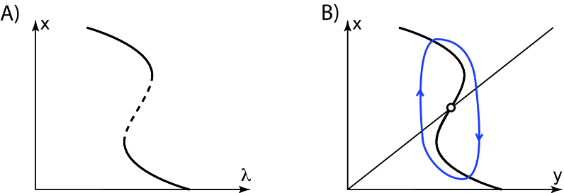
Figure 1: Relaxation oscillations in the universal unfolding of the hysteresis bifurcation. A. A persistent bifurcation diagram of the hysteresis singularity. Branches of stable (resp. unstable) fixed points are depicted as full (resp. dashed) lines. B. Through a slow adaptation of the bifurcation parameter, the bifurcation diagram in A. is transformed into the phase plane of a two-dimensional dynamical system, which still defines a universal unfolding of the hysteresis singularity. The thick full line is the fast subsystem nullcline. The thin full line is the slow subsystem nullcline. The circle denotes an unstable fixed point. For small $\beta>0$, the model exhibits exponentially stable relaxation oscillations (depicted in light blue).

Because $y$ is a slow variable, it acts as a slowly varying modulation of the bifurcation parameter in the fast dynamics (2.2a). As a consequence, the global analysis of system (2.2) reduces to a quasi-steady state bifurcation analysis of (2.2a), hence the relationship between Fig. 1A and Figure 1B.

The following (well known) theorem characterizes a global attractor of (2.2), that is the existence of Van-der-Pol type relaxation oscillations in the universal unfolding of the hysteresis.

Theorem 1

[Grasman1987],[Mishchenko1980],[Krupa2001c] For $\lambda=0$ and for all $0<\beta<1$, there exists $\bar{\varepsilon}>0$ such that, for all $\varepsilon\in(0,\bar{\varepsilon}]$, the dynamical system (2.2) possesses an exponentially stable relaxation limit cycle, which attracts all solutions except the equilibrium at $(0,0)$.

The familiar reader will recognize in (2.2) a famous model of neurodynamics introduced by FitzHugh [FitzHugh1961]. It is the prototypical planar reduction of spiking oscillations. There is therefore a close relationship between the hysteresis singularity and spike generation.

It is worth emphasizing that the relationship between singularity theory (Fig. 1A) and the two-time scale phase portrait (Fig. 1B) imposes choosing the bifurcation parameter, not an unfolding parameter, as the slow variable. It should also be observed that the slow variable is a deviation from the unfolding parameter $\lambda$ rather than the bifurcation parameter itself. Keeping $\lambda$ as the bifurcation parameter of the two-dimensional dynamics (2.2) allows to shape its equilibrium structure accordingly to the universal unfolding of the organizing singularity, in this case, the hysteresis, and will play an important role in the next section.

2.3 The winged cusp singularity and rest-spike bistability

We repeat the elementary construction of Section 2.2 for the codimension-3 winged cusp singularity $-x^{3}-\lambda^{2}$. It differs from the hysteresis singularity in the non-monotonicity of $g(x,\lambda)$ in the bifurcation parameter, that is $\frac{\partial(-x^{3}-\lambda^{2})}{\partial\lambda}=-2\lambda$ changes sign at the singularity.

Figure 2A illustrates an important persistent bifurcation diagram in the unfolding of the winged cusp, obtained for $\gamma=0$, $\beta>0$, and $\alpha<-2\left(\frac{\beta}{3}\right)^{3/2}$. We call it the mirrored hysteresis bifurcation diagram. The right part ($\lambda>0$) of this bifurcation diagram is essentially the persistent bifurcation diagram of the hysteresis singularity in Figure 1A. In that region, $\frac{\partial G_{wcusp}^{s}}{\partial\lambda}<0$. The left part ($\lambda>0$) is the mirror of the hysteresis and, in that region, $\frac{\partial G_{wcusp}^{s}}{\partial\lambda}>0$. For $\gamma\neq 0$, the mirroring effect is not perfect, but the qualitative analysis does not change. The hysteresis and its mirror collide in a transcritical singularity for $\alpha=-2\left(\frac{\beta}{3}\right)^{3/2}$. This singularity belongs to the transcritical bifurcation transition variety in the winged cusp unfolding (see Appendix LABEL:SEC:_trans_variety). The transcritical bifurcation variety plays an important role in the forthcoming analysis.

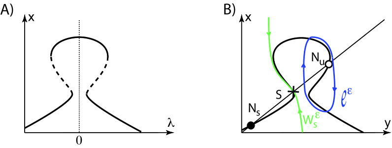
Figure 2: Singularly perturbed rest-spike bistability in the universal unfolding of the winged cusp. A. Mirrored hysteresis persistent bifurcation diagram of the winged cusp for $\beta>0$, $\alpha<-2\left(\frac{\beta}{3}\right)^{3/2}$, and $\gamma=0$. B. A phase plane of (2).

We use the algebraic curve in Figure 2A to generate the phase portrait in Figure 2B of the two-dimensional model rCl ˙x&=G_wcusp^s(x,λ+y; α,β,γ)
=-x^3+βx-(λ+y)^2-γ(λ+y)x -α
˙y=ε(x-y). Its fixed point equation

$$F(x,\lambda,\alpha,\beta,\gamma):=-x^{3}+\beta x-(\lambda+x)^{2}-\gamma(\lambda+x)x-\alpha.$$ (6)

is easily shown to be again a universal unfolding of the winged cusp around $x_{wcusp}:=\frac{1}{3}$, $\lambda_{wcusp}:=0$, $\alpha_{wcusp}:=-\frac{1}{27}$, $\beta_{wcusp}:=-\frac{1}{3}$, $\gamma_{wcusp}:=-2$. The face portrait in Fig. 2B is a prototype phase portrait of rest-spike bistability: a stable fixed point coexists with a stable relaxation limit cycle.

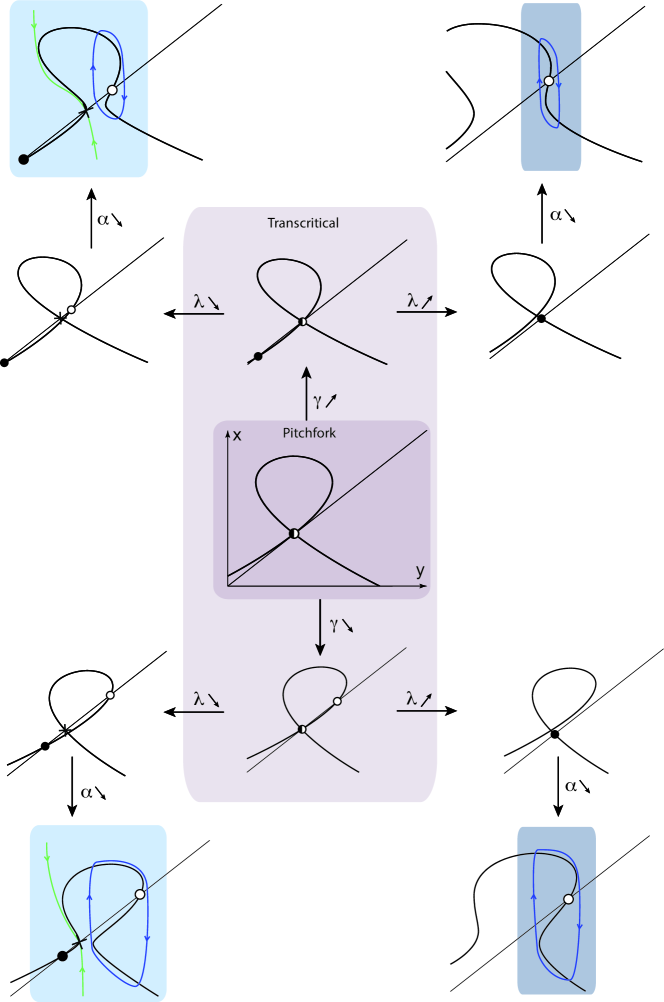
Figure 3: An unfolding of the pitchfork bifurcation variety in (2). The phase portraits in Figs. 1 and 2 both belong to the unfolding of the pitchfork singularity in center. A smooth deformation of the phase portrait of Fig. 1 into the phase portrait of Fig. 2 involves a transcritical bifurcation, which degenerate into a pitchfork for a particular value of the unfolding parameter $\gamma$

.

Similarly to the previous section, the analysis of the singularly perturbed model (2) is completely characterized by the bifurcation diagram of Figure 2A. This bifurcation diagram provides a skeleton for the rest-spike bistable phase portrait in Figure 2B, as stated in the following theorem. Its proof is provided in Section LABEL:SSEC:_cusp_bist_proof.

Theorem 2

For all $\beta>\beta_{wcusp}$, there exist open sets of bifurcation ($\lambda$) and unfolding ($\alpha,\gamma$) parameters near the pitchfork singularity at $(\lambda,\alpha,\gamma)=(\lambda_{PF}(\beta),\alpha_{PF}(\beta),\gamma_{PF}(\beta))$, in which, for sufficiently small $\varepsilon>0$, model (2) exhibits the coexistence of an exponentially stable fixed point $N_{s}$ and an exponentially stable spiking limit cycle $\ell^{\varepsilon}$. Their basins of attraction are separated by the stable manifold $W_{s}^{\varepsilon}$ of a hyperbolic saddle $S$ (see Fig. 2B).

Figure 3 shows the transition in (2) from the hysteresis phase portrait in Figure 1B to the bistable phase portrait in Fig. 2B through a transcritical bifurcation. Both phase portraits are generated by unfolding the degenerate portrait in Fig. 3, center, which belongs to the pitchfork bifurcation variety $(\alpha,\gamma)=(\alpha_{PF}(\beta),\gamma_{PF}(\beta))$, $\beta>\beta_{wcusp}$ (see Appendix LABEL:SEC:_trans_variety). The transcritical bifurcation variety $\alpha=\alpha_{TC}(\beta,\gamma)$ is obtained through variations of the unfolding parameter $\gamma$ away from the pitchfork variety. It provides the two phase portraits in Fig. 3, center top and bottom. By increasing or decreasing the bifurcation parameter $\lambda$ and decreasing the unfolding parameter $\alpha$ out of the transcritical bifurcation variety, these phase portraits perturb to the generic phase portraits in the corner, corresponding to the qualitative phase portraits in Figures 1B and Fig. 2B, respectively. The reader of [Franci2012] will recognize the same organizing role of the pitchfork in a planar model of neuronal excitability.

2.4 A three-time scale bursting attractor in the winged cusp unfolding

The coexistence of a stable resting state and stable spiking oscillation, or singularly perturbed rest-spike bistability, makes (2) a good candidate as the slow-fast subsystem of a three-time scale minimal bursting model: rCl ˙x&=G_wcusp^s(x,λ+y; α+z,β,γ)
=-x^3+βx-(λ+y)^2-γ(λ+y)x -α-z
˙y=ε_1(x-y)
˙z=ε_2 (-z + a x+b y + c ), where $0<\varepsilon_{2}\ll\varepsilon_{1}\ll 1$ and $a,b,c\in\mathbb{R}$. The $z$-dynamics models the ultra-slow adaptation of the affine unfolding parameter $\alpha$, in such a way that the global attractor of (2.4) will be determined by a quasi-static modulation of (2.4a) through different persistent bifurcation diagrams.

Here, again, the role of singularity theory in distinguishing bifurcation and unfolding parameters is crucial. The hierarchy between these parameters and the state variable, formalized in the theory in [Golubitsky1985, Definition III.1.1], is reflected here in the hierarchy of timescales.

The time scale separation between (2.4a-2.4b) and (2.4-c) makes it possible once again to derive a global analysis of model (2.4) from the analysis of the steady state behavior of (2) as $\alpha$ is varied. Such analysis can easily be derived geometrically in the singular limit $\varepsilon_{1}=0$. It is sketched in Figure 4. For $\alpha\in(\alpha_{SN},\alpha_{SH}^{0})$, the singularly perturbed model (2) exhibits rest-spike bistability, that is, the coexistence of a stable node $N_{s}$, a singular stable periodic orbit $\ell^{0}$, and a singular saddle separatrix $W_{s}^{0}$. At $\alpha=\alpha_{SH}^{0}=-2\left(\frac{\beta}{3}\right)^{3/2}$ the left and right branches of the mirrored hysteresis bifurcation collide in a transcritical singularity that serves as a connecting point for a singular homoclinic trajectory $SH^{0}$. For $\alpha>\alpha_{SH}^{0}$, the only (singular) attractor is the stable node $N_{s}$. At $\alpha=\alpha_{SN}$, the saddle and the stable node merge in a saddle-node bifurcation $SN$. For $\alpha<\alpha_{SN}$, the only attractor is the singular periodic orbit $\ell^{0}$. The different singular invariant sets in Figure 4A, can be glued together to construct the three-dimensional singular invariant set $\mathcal{M}_{0}$ in Figure 4B-left.

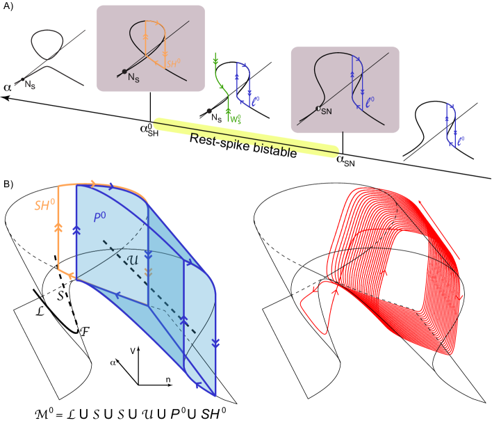
Figure 4: Singular steady-state behavior of (2) through a variation of the unfolding parameter $\alpha$. A. Singular phase portraits of (2) for $\gamma=0$, $\beta=\frac{1}{3}$, and small negative $\lambda$. B. Gluing the different invariant sets in A leads to the three-dimensional singular invariant set $\mathcal{M}^{0}$ (left), which provides a skeleton for a three-time scale bursting attractor (right) in the singularly perturbed system (2.4). The branch of stable fixed points (resp. saddle point) for $\alpha<\alpha_{SN}$ is drawn as the black solid curve $\mathcal{L}$ (resp. the black dashed curve $\mathcal{S}$). The saddle node bifurcation connecting them is denoted by $\mathcal{F}$. The branch of unstable fixed points is drawn as the black dashed line $\mathcal{U}$. The branch of stable singular periodic orbit for $\alpha<\alpha_{SH}^{0}$ is drawn as the blue cilindric surface $P^{0}$. The singular saddle homoclinic trajectory is drawn as the orange oriented curve $SH^{0}$.

The singular invariant set $\mathcal{M}_{0}$ provides a skeleton for a three-time scale bursting attractor that shadows the branch $\mathcal{L}$ of stable fixed points in alternation with the branch $P^{0}$ of (singular) stable periodic orbits, as depicted in Figure 4B-right. To prove the existence of such an attractor, we only need to understand how $\mathcal{M}^{0}$ perturbs for $\varepsilon_{1}>0$.

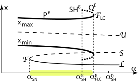
Figure 5: Bifurcation diagram of (2) with respect the unfolding parameter $\alpha$ for sufficiently small $\varepsilon$. The branch of stable fixed point is depicted as the full thin line $\mathcal{L}$, the branch of saddle point as the dashed thin line $\mathcal{S}$, and the branch of unstable fixed point as the dashed thin line $\mathcal{U}$. The branch of stable periodic orbit is depicted by the thick full lines $P^{\varepsilon}$ and the branch of unstable periodic orbits by the thick dashed lines $Q^{\varepsilon}$. $SH^{\varepsilon}$: saddle-homoclinic bifurcation. $\mathcal{F}_{LC}$: fold limit cicle bifurcation. $\mathcal{F}$: fold (saddle-node) bifurcation. The yellow strip between the saddle-node and fold limit cicle bifurcation denotes the rest-spike bistable range.

Near the singular limit, the branch of singular periodic orbits $P^{0}$ perturbs to a nearby branch of exponentially stable periodic orbits $P^{\varepsilon}$ (see Fig. 5), whereas the singular homoclinic trajectory $SH^{0}$ perturbs to an unstable homoclinic trajectory $SH^{\epsilon}$ (at $\alpha=\alpha_{SH}^{\epsilon}$). The branch of unstable periodic orbits $Q^{\varepsilon}$ generated at $SH^{\varepsilon}$ eventually merges with $P^{\varepsilon}$ at a fold limit cycle bifurcation $\mathcal{F}_{LC}$ for some $\alpha_{FLC}^{\varepsilon}\in(\alpha_{SH}^{\epsilon},\alpha_{SH}^{0})$. In the whole range $(\alpha_{SN},\alpha_{FLC}^{\varepsilon})$, model (2) exhibits the coexistence of a stable fixed point and a stable spiking limit cycle. The details of this analysis are contained in Lemma LABEL:LEM:_cusp_SH in Section LABEL:SSUB:_burst_att_proof.

We follow [Terman1991, Su2004] to derive conditions on the bifurcation and unfolding parameters in (2.4a-2.4b) and to place the hyperplane $\dot{z}=0$ (through a suitable choice of the parameters $a,b,c\in\mathbb{R}$) such that an ultra-slow variation of $z$ can hysteretically modulate the slow-fast subsystem (2.4a-2.4b) across its bistable range $(\alpha_{SN},\alpha_{FLC}^{\varepsilon})$ to obtain stable bursting oscillations. The existence of such bursting oscillations is stated in the following theorem. Its proof is provided in Section LABEL:SSUB:_burst_att_proof.

Theorem 3

For all $\beta>\beta_{wcusp}$, there exists an open set of bifurcation ($\lambda$) and unfolding ($\alpha,\gamma$) parameters near the pitchfork singularity at $(\lambda,\alpha,\gamma)=(\lambda_{PF}(\beta),\alpha_{PF}(\beta),\gamma_{PF}(\beta))$ such that, for all $\lambda,\alpha,\gamma$ in those sets, there exist $a,b,c,\in\mathbb{R}$ such that, for sufficiently small $\varepsilon_{1}\gg\varepsilon_{2}>0$, model (2.4) has a hyperbolic bursting attractor.

Theorem 3 uses the two regenerative phase portraits in Fig. 3 left to construct a bursting attractor by modulating the unfolding parameter $\alpha$. The bursting attractor directly rests upon the bistability of those phase portraits. It should be noted that the same construction can be repeated on the restorative phase portraits in Fig. 3 right. However those phase portraits are monostable and their ultra-slow modulation leads to a slow tonic spiking (i.e. a single spike necessarily followed by a rest period). This attractor differs from a bursting attractor by the absence of a bistable range in the bifurcation diagrams of Fig. 4. It can be shown that the persistence of (rest-spike) bistability in the singular limit is a hallmark of regenerative excitability (Fig. 3 left) and that it cannot exist in restorative excitability (Fig. 3 right). See [Franci2013] for a mode detailed discussion. Modulation in (2.4) of the bifurcation parameter across the transcritical bifurcation of Fig. 3 therefore provides a geometric transition from the slow tonic spiking attractor to the bursting attractor. This transition organizes the geometric route into bursting discussed in the next section.

3 A physiological route to bursting

3.1 A minimal three-time scale bursting model

The recent paper [Franci2012] introduces the planar neuron model rCl ˙V&=V-V33-n^2+I
˙n=ε(n_∞(V-V_0)+n_0-n) Its phase portrait was shown to contain the pitchfork of Figure 3 as an organizing center, leading to distinct types of excitability for distinct values of the unfolding parameters. The analysis of the previous section suggests that a bursting model is naturally obtained by augmenting the planar model (3.1) with ultra slow adaptation: rCl ˙V&=kV-V33-(n+n_0)^2+I-z
˙n=ε_n(V)(n_∞(V-V_0) -n )
˙z=ε_z(V)(z_∞(V-V_1)-z) Model (3.1) is essentially model (3.1) for $k=1$ and $z=0$, modulo a translation $n\leftarrow n+n_{0}$. The dynamics (3.1b-3.1c) mimic the kinetics of gating variables in conductance-based models, where the steady-state characteristics $n_{\infty}(\cdot)$ and $z_{\infty}(\cdot)$ are monotone increasing (typically sigmoidal) and the time scaling $\varepsilon_{n}(\cdot)$ and $\varepsilon_{z}(\cdot)$ are Gaussian-like strictly positive functions. Details of model (3.1) for the numerical simulations of the paper are provided in Appendix LABEL:SEC:_parameters.

The slow-fast subsystem (3.1a3.1b) shares the same geometric structure as (2). After a translation $V\leftarrow V+V_{0}$, the right hand side of (3.1a) can easily be shown to be a universal unfolding of the winged cusp and the slow dynamics (3.1b) modulates its bifurcation parameter. Plugging the ultra-slow dynamics (3.1c), one recovers the same structure as (2.4). Therefore, the conclusions of Theorems 2 and 3 apply to (3.1).

The difference between (3.1) and (2.4) is that the model (3.1) has the physiological interpretation of a reduced conductance-based model, with $V$ a fast variable that aggregates the membrane potential with all fast gating variables, $n$ a slow recovery variable that aggregates all the slow gating variables regulating neuronal excitability, and $z$ an ultra-slow adaptation variable that aggregates the ultra-slow gating variables that modulate the cellular rhythm over the course of many action potentials. Finally, $I$ models an external applied current.

3.2 Model parameters and their physiological interpretation

The bifurcation parameter $n_{0}$ models the balance between restorative and regenerative ion channels

The central role of the bifurcation parameter $n_{0}$ in (3.1) was analyzed in [Franci2012, Franci2013] and is illustrated in Fig. 6. The transcritical bifurcation variety in Fig. 3 corresponds to the physiologically relevant transition from restorative excitability (large $n_{0}$) to regenerative excitability (small $n_{0}$). When the excitability is restorative, the recovery variable $n$ provides negative feedback on membrane potential variations near the resting equilibrium, a physiological situation well captured by FitzHugh-Nagumo model (or the hysteresis singularity). In contrast, when excitability is regenerative, the recovery variable $n$ provides positive feedback on membrane potential variations near the resting potential, a physiological situation that requires the quadratic term in (3.1a) (or the winged cusp singularity).

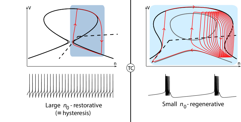
Figure 6: Transition from restorative excitability (tonic firing) to regenerative excitability (bursting) in model (3.1) by sole variation of the bifurcation parameter $n_{0}$. The analytical expression of the steady state functions $n_{\infty}(\cdot)$ and $z_{\infty}(\cdot)$ and numerical parameter values are provided in Appendix LABEL:SEC:_parameters. The time scale is the same in the left and right time series.

The value of $n_{0}$ in a conductance-based model reflects the balance between restorative and regenerative ion channels that regulate neuronal excitability. How to determine the balance in an arbitrary conductance-based model is discussed in [Franci2013]. Note that the restorative or regenerative nature of a particular ion channel in the slow time-scale is an intrinsic property of the channel. A prominent example of restorative channel is the slow potassium activation shared by (almost) all spiking neurons. A prominent example of regenerative channel is the slow calcium activation encountered in most bursting neurons. The presence of regenerative channels in neuronal bursters is well established in neurophysiology. See e.g. [Krahe2004, Astori2011].

The affine unfolding parameter provides bursting by ultra-slow modulation of the current across the membrane

For small $n_{0}$, the modulation of the ultra-slow variable $z$ creates a hyperbolic bursting attractor through the hysteretic loop described in Fig. 4. The burster becomes a single-spike limit cycle (tonic firing) for large $n_{0}$ (restorative excitability), that is, in the absence of rest-spike bistability in the planar model.

The presence of ultra-slow currents in neuronal bursters is well established in neurophysiology (see e.g. [Astori2011]). A prominent example is provided by ultra-slow calcium activated potassium channels.

Half activation potential affects the route to bursting

The role of the unfolding parameter $\gamma$ in (2.4) is illustrated in Fig. 3: it provides two qualitatively distinct paths connecting the restorative and regenerative phase portraits. This role is played by the parameter $V_{0}$ in the planar model (3.1) studied in [Franci2012], which has the physiological interpretation of a half activation potential. The role of half-activation potentials in neuronal excitability is well documented in neurophysiology (see e.g. [Putzier2009]). The role of this unfolding parameter in the route to bursting is discussed in the next subsection.

No spike without fast autocatalytic feedback

The role of the unfolding parameter $k$ in (3.1) is to provide positive (autocatalytic) feedback in the fast dynamics. The prominent source of this feedback in conductance-based models is the fast sodium activation. It is well acknowledged in neurodynamics [Izhikevich2007].

The reduced model (3.1) makes clear predictions about its dynamical behavior in the absence of this feedback (i.e. $k=0$). Those predictions are further discussed in Section LABEL:SSEC:_burst_across_bursting_types and are in closed agreement with the experimental observation of “small oscillatory potentials” when sodium channels are shut down with pharmacological blockers [Guzman2009, Zhan1999] or are poorly expressed during neuronal cell development [Liu1998].

3.3 A physiological route to bursting

A central insight of the reduced model (3.1) is that it provides a route to bursting: fixing all unfolding parameters and varying only the bifurcation parameter $n_{0}$ leads to a smooth transition from tonic firing to bursting, see Fig. 7.

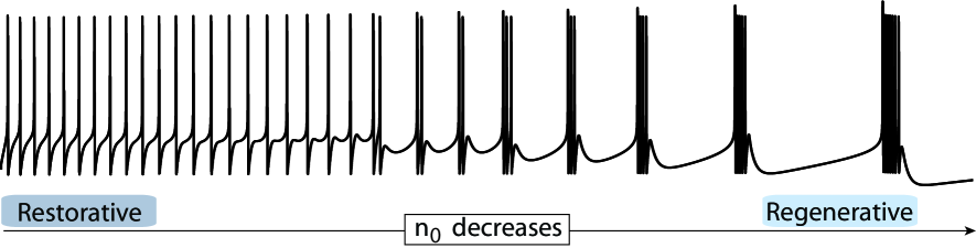
Figure 7: Route from tonic firing to bursting in model (3.1) via a smooth variation of the bifurcation parameter $n_{0}$. Rest of the parameter as in Figure 6.

Smooth and reversible transitions between those two rhythms have been observed in many experimental recordings [Sherman2001, Viemari2006], making the route to burst an important signaling mechanism. The fact that the modulation is achieved simply through the bifurcation parameter $n_{0}$, i.e. the balance between restorative and regenerative channels, is of physiological importance because it is consistent with the physiology of experimental observations of routes into bursting [Sherman2001, Viemari2006, Beurrier1999].

The analysis in the above sections shows that the transition from single spike to bursting is through the transcritical bifurcation variety in model (2). Looking at the singular limit $\varepsilon=0$ of (2) near this transition variety provides further insight on the geometry of the route that leads to the appearance of the saddle-homoclinic bifurcation organizing the bistable phase-portrait. This route is organized by the path through the pitchfork bifurcation, which provides the most symmetric path across the transcritical variety. The generic transitions are understood by perturbing the degenerate path.

Fig. 8A shows the qualitative projection of those paths onto the $(V_{0},n_{0})$ parameter chart obtained in model (3.1) for $I=\frac{2}{3}$. The chart is reproduced from [Franci2012]. The same qualitative picture is obtained for the $(\gamma,\lambda)$ parameter chart of the abstract model (2) at $\alpha=\alpha_{TC}(\beta,\gamma)$ (see Appendix LABEL:SEC:_trans_variety). The chart associates different excitability types (as well as their restorative or regenerative nature, see [Franci2013]) to distinct bifurcation mechanisms. Unfolding those paths along the $I$ (or $\alpha$) direction leads to the bifurcation diagrams in Fig. 9B. They reveal (in the singular limit) the onset of the bistable range organized by the singular saddle-homoclinic loop $SH^{0}$ as paths cross the transcritical bifurcation variety.

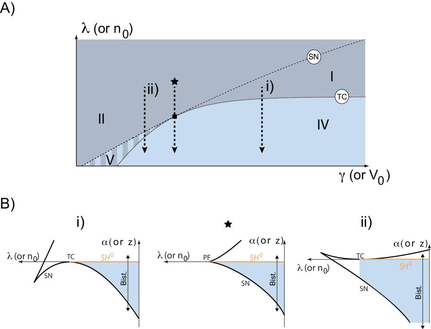
Figure 8: Routes into bursting in the universal unfolding of the pithfork bifurcation. A. Qualitative projection of routes into bursting onto the $(V_{0},n_{0})$ (resp. $(\gamma,\lambda)$) of model (3.1) (resp. (2)) for $I=\frac{2}{3}$ (resp. $\alpha=\alpha_{TC}(\beta,\gamma)$, see Appendix LABEL:SEC:_trans_variety). Excitability is restorative in subregions $I$ and $II$, mixed in subregion $V$, and regenerative in subregion $IV$. See [Franci2012] and [Franci2013] for details concerning the underlying bifurcation mechanisms. The transition path labeled with a star depicts the degenerate path across the pitchfork. The generic paths i) and ii) are distinguished by different half activation potentials $V_{0}$ (resp. unfolding parameter $\gamma$). B. Unfolding of transition paths in A along the $I$ (resp. $\alpha$) direction. Black thick lines denote branches of saddle-node (SN) bifurcation. In paths i) and ii), the model undergoes a transcritical bifurcation (TC) as the path touches tangentially a branch of SN bifurcations. In the degenerate path, the model undergoes a pitchfork (PF) bifurcation as the path enters the cusp tangentially to both branches of SN bifurcations. The singular saddle-homoclinic loop, geometrically constructed in Figs. 4 and 9, is denoted by $SH^{0}$ and determines the appearance of a singular bistable range persisting away from singular limit.

The same qualitative picture persists for $\varepsilon>0$. Fig. 9 illustrates how the appearance of the singular saddle-homoclinic loop is accompanied, for $\varepsilon>0$, by a smooth transition from a monostable (SNIC - route i) ) or barely bistable (sub. Hopf - route ii) ) bifurcation diagram to the robustly bistable bifurcation diagram constructed in the sections above (Fig. 5). Through ultra-slow modulation of the unfolding parameter $\alpha$, this transition geometrically captures the transition from tonic spiking to bursting via the sole variation of the bifurcation parameter.

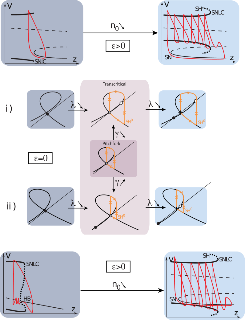
Figure 9: Geometry of the two generic routes into bursting in the unfolding of the pitchfork bifurcation in model (2.4) and model (3.1).

The strong agreement between the mathematical insight provided by singularity theory and the known electrophysiology of bursting is a peculiar feature of the proposed approach. There is a direct correspondence between the bifurcation and unfolding parameters of the winged cusp and the physiological minimal ingredients of a neuronal burster. In particular, our analysis predicts that any bursting neuron must possess at least one physiologically regulated slow regenerative channel. This prediction needs to be tested systematically but we have found no counter-example in the bursting neurons we have analyzed to date.

4 Normal form reduction of conductance-based models

4.1 A two dimensional reduction

The winged cusp singularity emerges as an organizing center of rhythmicity in the reduced neuronal model (3.1), but a legitimate question is whether this singularity can be traced in arbitrary (high-dimensional) conductance-based models. Our recent paper [Franci2013] addresses a closely related question for the transcritical variety. It provides an analog of the bifurcation parameter $n_{0}$ in arbitrary conductance-based models of the form rCll C_m˙V&=-∑_ι¯g_ιm_ι^a_ι h_ι^b_ι (V-E_ι)+I_app,
=:I_ion(V,x^f,x^s,x^us)+I_app
τ_x^f_j(V)˙x^f_j=-x^f_j+x^f_j,∞(V), j=1,…,n_f
τ_x^s_j(V)˙x^s_j=-x^s_j+x^s_j,∞(V), j=1,…,n_s
τ_x^us_j(V)˙x^us_j=-x^us_j+x^us_j,∞(V), j=1,…,n_us where $\iota$ runs through all ionic currents, $x^{f}:=[x^{f}_{j}]_{j=1,\ldots,n_{f}}$ denotes the $n_{f}$-dimensional column vector of fast gating variables, $x^{s}:=[x^{s}_{j}]_{j=1,\ldots,n_{s}}$ denotes the $n_{s}$-dimensional column vector of slow gating variables, and $x^{us}:=[x^{us}_{j}]_{j=1,\ldots,n_{us}}$ denotes the $n_{us}$-dimensional column vector of ultra-slow variables (see also [Franci2013] for more details on the adopted notation).

Following common analysis methods in neurodynamics, we want to reduce the (possibly) high-dimensional model (4.1) to a two-dimensional model of the form rCl ˙V &=F(V,n)+I
τ(V)˙n^s=-n+n_∞^s(V) where $V$ is the fast voltage and $n$ is a slow aggregate variable. We achieve this reduction by first considering the singular limit of three time scales leading to a quasi-steady state approximation for fast gating variables, that is

$$x^{f}_{j}\equiv x^{f}_{j,\infty}(V),$$ (7)

for all $j=1,\ldots,n_{f}$, and freezing ultra-slow variables, that is setting

$$x^{us}_{j}\equiv\bar{x}^{us}_{j},$$

for all $j=1,\ldots,n_{us}$, where the values $\bar{x}^{us}_{j}$ belong to the physiological range of the different variables. The remaining dynamics read as rCl˙V&=I_ion(V,x^f_∞(V),x^s,¯x^us)+I_app,
τ(V)˙x^s_j=(-x^s_j+x^s_j,∞(V)), j=1,…,n_s which is a fast-slow system with $V$ as fast variable and $x^{s}$ as slow variables.

The planar reduction proceeds from the change of variables rCln&=x_1