A sample of relatively unstudied star clusters in the Large Magellanic Cloud: fundamental parameters determined from Washington photometry

Abstract

Aims. To enlarge our growing sample of well-studied star clusters in the Large Magellanic Cloud (LMC), we present CCD Washington $CT_{1}$ photometry to $T_{1}\sim$ 23 in the fields of twenty-three mostly unstudied clusters located in the inner disc and outer regions of the LMC.

Methods. We estimated cluster radii from star counts. Using the cluster Washington $(T_{1},C-T_{1})$ colour-magnitude diagrams, statistically cleaned from field star contamination, we derived cluster ages and metallicities from a comparison with theoretical isochrones of the Padova group. Whenever possible, we also derived ages using $\delta T_{1}$ - the magnitude difference between the red giant clump and the main sequence turn off - and estimated metallicities from the standard giant branch procedure. We enlarged our sample by adding clusters with published ages and metallicities determined on a similar scale by applying the same methods. We examined relationships between their positions in the LMC, ages and metallicities.

Results. We find that the two methods for age and metallicity determination agree well with each other. Fourteen clusters are found to be intermediate-age clusters (1-2 Gyr), with [Fe/H] values ranging from -0.4 to -0.7. The remaining nine clusters turn out to be younger than 1 Gyr, with metallicities between 0.0 and -0.4.

Conclusions. Our 23 clusters represent an increase of $\sim$ 30% in the current total amount number of well-studied LMC clusters using Washington photometry. In agreement with previous studies, we find no evidence for a metallicity gradient. We also find that the younger clusters were formed closer to the LMC centre than the older ones.

1 Introduction

The Large Magellanic Cloud (LMC) has become one of the most-studied objects in the past three decades. In particular, studying the LMC star cluster system advances our understanding of the chemical enrichment and star-formation history of this galaxy as a whole (e.g., Baumgardt et al. 2012), with the important caveat that a large portion of the LMC’s history cannot be studied via clusters because of the infamous age gap (Geisler et al. 1997). However, the number of well-studied clusters in the LMC still constitutes a very small fraction of those that have been catalogued, and thorough investigations of even a handful of clusters can significantly improve our knowledge of the chemical enrichment history of this critical galaxy.

The current study represents a step forward in the systematic study of LMC clusters carried out as uniformly as possible using the Washington photometric system. Although initially developed for late-type stars and old stellar populations (Canterna 1976), the Washington system has been widely applied to intermediate-age and old clusters in the Galaxy and in the Magellanic Clouds (e.g., Geisler et al. 1997; Geisler & Sarajedini 1999; Piatti et al. 2003b; Piatti 2012b). It is our purpose to derive ages and metallicities for a sample of 23 mostly unstudied LMC star clusters with the aim of adding them to our growing sample of well-studied clusters. The reasons why we have chosen to work in this photometric system and its advantages for this type of study have already been described in previous papers (e.g., Geisler et al. 1997; Piatti et al. 2011).

The cluster sample is presented in Section 2. The observations and reductions are described in Section 3. The procedure followed to estimate cluster radii from the stellar density profiles is described in Section 4. We also include in this section the method applied to minimize the field-star contamination in the Washington $(T_{1},C-T_{1})$ colour-magnitude diagrams (CMDs) and the estimation of the cluster fundamental properties. A brief analysis and discussion of the results is presented in Section 5, while Sect. 6 summarizes our results.

2 Cluster sample

After a careful revision of the Washington wide-field images of 21 LMC regions (see Section 3), we selected those star clusters located outside the bar for the present study that appeared to be unstudied or were only poorly studied. Our final sample includes a total of 23 mostly unstudied clusters, eleven of which lie in the inner disc of the LMC but outside the bar. The remaining twelve are located in the outer region (Fig. 1). Here we adopt the definition presented in Bica et al. (1998) in the sense that the inner disc is that region where the mean field turnoff becomes as bright as the clump. This takes place at a deprojected radius of $\sim$ 4^∘. The cluster sample is presented in Table 1, where we list the various star cluster designations from different catalogues (column 1), 2000.0 equatorial and galactic coordinates (columns 2-5), and the cluster radii given in Bica et al. (2008) (column 6). These radii constitute half of the mean apparent diameters obtained by computing the average between the major (a) and minor (b) axes. The last two columns of Table 1 (columns 7,8) list the cluster radii derived in the current study in pixels and parsecs, respectively (see Section 4.1).

Table 1: Observed star clusters in the LMC.

Star cluster	$\alpha_{2000}$	$\delta_{2000}$	l	b	r	rcls	rcls
	(h m s)	($\circ$ ’ ”)	($\circ$)	($\circ$)	(’)	(px)	(pc)
SL 33, LW 59, KMHK 91	04 46 25	-72 34 06	284.717	-34.986	0.55	200	13.1
SL 41, LW 64, KMHK 105	04 47 30	-72 35 18	284.704	-34.903	0.72	220	14.4
KMHK 123	04 49 00	-72 38 24	284.713	-34.780	0.30	110	7.2
KMHK 128	04 49 14	-72 03 24	285.177	-34.613	0.26	110	7.2
LW 69, KMHK 137	04 49 39	-72 14 53	284.246	-34.874	0.32	120	7.8
KMHK 151	04 50 21	-72 49 39	284.881	-34.619	0.27	170	11.1
SL 54, LW 78, KMHK 162	04 50 48	-72 34 36	284.582	-34.677	0.55	200	13.1
SL 73, LW 86, KMHK 214	04 52 45	-72 31 04	284.454	-34.561	0.34	190	12.4
SL 72, LW 87, KMHK 217	04 52 54	-72 10 21	284.054	-34.667	0.42	160	10.5
BSDL 594, LOGLE 87	05 05 53	-67 02 58	277.678	-35.039	0.42	140	9.2
BSDL 654,LOGLE 123	05 07 21	-66 49 45	277.377	-34.949	0.22	75	4.9
BSDL 665, LOGLE 130	05 07 47	-66 47 53	277.329	-34.914	0.22	60	3.9
BSDL 675, LOGLE 134	05 07 56	-67 21 28	277.990	-34.776	0.29	90	5.9
HS 130, KMHK 588	05 09 15	-67 41 59	278.362	-34.577	0.27	90	5.9
BSDL 761	05 10 02	-66 41 57	277.155	-34.717	0.32	90	5.9
BSDL 779, LOGLE 182	05 10 32	-66 56 24	277.428	-34.619	0.22	80	5.2
HS 156, H88-190, KMHK 632, LOGLE 199	05 11 11	-67 37 36	278.227	-34.414	0.25	120	7.8
HS 178, KMHK 667	05 13 48	-66 37 12	276.970	-34.367	0.33	120	7.8
LW 211, KMHK 901	05 25 27	-73 34 13	284.858	-31.979	0.33	160	10.5
C11	05 50 48	-71 42 28	282.371	-30.397	0.20	150	9.8
BSDL 3158	05 52 11	-71 51 30	282.533	-30.276	0.46	220	14.4
KMHK 1702	06 13 56	-72 30 19	283.190	-28.586	0.31	100	6.5
SL 870, LW 440, KMHK 1705	06 14 28	-72 36 34	283.310	-28.546	0.58	230	15.0

Figure 1: Position of our target clusters (open circles) in relation to the LMC bar (dashed lines) and geometrical centre (cross). (1) SL,33, (2) SL 41, (3) KMHK 123, (4) KMHK 128, (5) LW 69, (6) KMHK 151, (7) SL 54, (8) SL 73, (9) SL 72, (10) BSDL 594, (11) BSDL 654, (12) BSDL 665, (13) BSDL 675, (14) HS 130, (15) BSDL 761, (16) BSDL 779, (17) HS 156, (18) HS 178, (19) LW 211, (20) C 11, (21) BSDL 3158, (22) KMHK 1702, (23) SL 870.

3 Data collection and reduction

The observations of the selected clusters were carried out with the “Víctor Blanco” 4-m telescope at Cerro Tololo Inter-American Observatory (CTIO, Chile), during the nights of 2000 December 29 and 30. Washington wide-field images of about 21 LMC regions were taken with the MOSAIC II camera, which consists of an 8K$\times$8K CCD detector array. One pixel of the MOSAIC wide-field camera subtends 0.27” on the sky, resulting in a 36’$\times$36’ field of view. We used the Washington C (Canterna 1976) and Kron-Cousins R filters to be consistent with our previous studies. As shown in Geisler (1996), the R filter has a significantly higher throughput than the standard Washington $T_{1}$ filter, so that R magnitudes can be accurately transformed to yield $T_{1}$ magnitudes. In particular, this filter combination allowed us to derive accurate metallicities based on the standard giant branch method described in Geisler & Sarajedini (1999). The Washington C and Kron-Cousins R filters were used with typical exposure times of 450 and 150 seconds, respectively. We obtained a series of bias, dome, and sky flat-field exposures per filter to calibrate the CCD instrumental signature. Standard stars of selected areas SA 98 and SA 101 from the list in Geisler (1996) were also nightly observed to standardize our photometry. SA 98 and SA 101 contain 15 and 9 standard stars, respectively, with a wide range in colour.

The MOSAIC data were reduced using the MSCRED package within IRAF following the guide for mosaic reduction of Januzzi et al. (2003). Stellar photometry was performed using the stand-alone DAOPHOT II provided by Peter Stetson. For star-finding and point spread function (PSF) fitting routines, and to combine all independent measurements, we used the DAOPHOT, ALLSTAR, DAOMATCH, and DAOMASTER programs (Stetson 1987). The calibration between instrumental and standard magnitudes was obtained using the following equations:

$$c=a_{1}+(C-T_{1})+T_{1}+a_{2}X_{C}+a_{3}(C-T_{1}),$$ (1)

$$r=b_{1}+T_{1}+b_{2}X_{T_{1}}+b_{3}(C-T_{1}),$$ (2)

where X is the effective airmass. Upper and lower-case letters represent standard and instrumental magnitudes, respectively. The coefficients $a_{i}$ and $b_{i}$ were derived nightly through the IRAF routine FITPARAM. The resulting mean calibration coefficients together with their errors are shown in Table 2. The nightly rms errors from the transformation to the standard system were 0.006 and 0.007 mag for $C$ and $T_{1}$, respectively, indicating that the nights had excellent photometric quality. We finally used about 15 standard stars.

Table 2: Standard system mean calibration coefficients.

$C$	$T_{1}$
$a_{1}=(0.039\pm 0.013)$	$b_{1}=(-0.667\pm 0.011)$
$a_{2}=(0.249\pm 0.007)$	$b_{2}=(0.049\pm 0.006)$
$a_{3}=(-0.098\pm 0.003)$	$b_{3}=(-0.020\pm 0.003)$

The full information gathered for each cluster consists of a running star number, the CCD x and y coordinates, the derived $T_{1}$ magnitude and $C-T_{1}$ colour, and the photometric errors $\sigma(T_{1})$ and $\sigma(C-T_{1})$. The behaviour of the $T_{1}$ and $C-T_{1}$ errors as a function of $T_{1}$ for the field of BSDL 3158 is shown in Fig. 2. Only a portion of the Washington data obtained for the star cluster SL 33 is shown here (see Table 3) for guidance regarding their form and content. The entire dataset for all clusters can be obtained as supplementary material from the on-line version of the journal.

Figure 2: $T_{1}$ magnitude and $C-T_{1}$ colour photometric errors as a function of $T_{1}$ for stars measured in the field of BSDL 3158.

Table 3: CCD $CT_{1}$ data of all stars in the field of SL 33.

ID	x	y	$T_{1}$	$\sigma T_{1}$	$C-T_{1}$	$\sigma(C-T_{1})$
	(px)	(px)	(mag)	(mag)	(mag)	(mag)
100	10.893	2847.002	22.363	0.060	0.689	0.071
101	10.917	4041.597	21.874	0.038	1.165	0.064
102	11.043	1675.679	20.334	0.012	1.679	0.022
103	11.095	695.358	21.023	0.018	0.585	0.023
104	11.106	3709.245	21.308	0.022	0.679	0.029
105	11.135	3222.543	16.817	0.005	1.962	0.006
106	11.155	1742.405	21.034	0.022	0.725	0.028
107	11.211	723.802	21.527	0.025	0.670	0.035
108	11.345	2543.743	21.005	0.020	0.526	0.025
109	11.365	3961.926	21.809	0.035	0.943	0.050
110	11.677	1627.802	18.183	0.004	2.153	0.007

4 Data analysis

4.1 Cluster properties from star counts

To construct density profiles of the observed clusters, we began by fitting Gaussian distributions to the star counts in the x and y directions to determine the coordinates of the cluster centres and their estimated uncertainties. The number of stars projected along these two directions were counted using five-pixel intervals, thus allowing us to statistically sample the spatial distributions. The fit of a single Gaussian for each projected density profile was performed using the NGAUSSFIT routine in the STSDAS/IRAF package. The cluster centres were determined with a typical standard deviation of $\pm$5 pixels ($\sim$ 1.35”). In the particular cases in which clusters showed peculiar morphologies, like an elongation in one direction or a marked sparsity, the standard deviation turned out to be slightly higher ($\pm$10 pixels or $\sim$ 2.7”). This is the case of clusters LW 69, SL 72, BSDL 665, and BSDL 675. Although the determination of cluster centres in these cases includes a higher degree of uncertainty, this uncertainty does not significantly change the final value obtained for the cluster radius because of the clusters’ dimensions. We then built the cluster radial profiles by computing the number of stars per unit area at a given radius r, as shown in Fig. 3. The cluster radius (r_cls), defined as the distance from the cluster’s centre where the density of stars equals that of the background, is given in pixels in column 7 of Table 1. Column 8 of Table 1 lists the cluster linear radii in parsecs calculated assuming that LMC is located at a distance of 50 kpc (Subramanian & Subramaniam 2010).

Figure 3: Stellar density profiles for the selected clusters, with the Poisson errors included. The horizontal lines correspond to the background levels far from the clusters. The background level was determined by estimating the mean stellar density at distances larger than $\sim$ 300 pixels from the centre of each cluster.

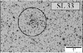
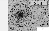
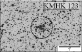
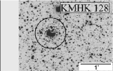
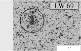
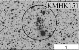
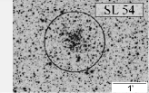
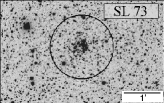
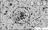
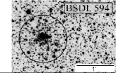
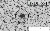
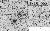
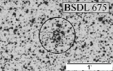
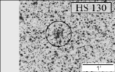
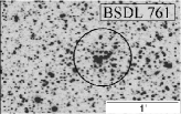
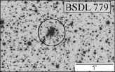
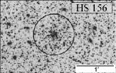
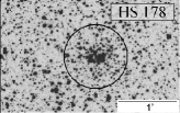
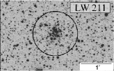
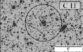
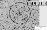
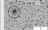
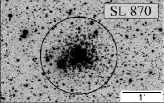
Figure 4: Schematic images of the stars observed in the fields of our target clusters. North is up and east is to the left. The circle in each figure has been drawn with the same radius (in pixels) as the radius obtained for each cluster.

4.2 Cluster properties from CMDs

We show in Fig. 4 schematic images of the stars observed in the cluster fields, while in Fig. 5 we show the $(T_{1},C-T_{1})$ CMD of all stars measured in the field of SL 41, which is one of the most populated fields observed. The remaining cluster fields exhibit CMDs whose features vary from one cluster to another, mainly depending on age.

Figure 5: Washington $(T_{1},C-T_{1})$ CMD for all the stars measured in the field of SL 41, one of the most populated clusters of our sample.

Since the fundamental cluster parameters estimation requires us to minimize the field-star contamination, we applied a statistical method recently developed in Piatti (2012a) that is described in detail in Piatti & Bica (2012). This procedure is briefly summarized as follows: It consists of selecting four field regions at a distance of between two and four times the cluster radius for each cluster. Then, their respective $(T_{1},C-T_{1})$ CMDs are obtained. The sizes of the areas of each field regions must be equal to the cluster area (generally taken as twice as large as the obtained cluster radius). Next, we count the stars lying within different intervals of magnitude-colour [$\delta T_{1},\delta(C-T_{1})$] in the CMD of each selected region. This new method includes variable intervals, depending on how populated the studied region is. The intervals happen to be bigger in more “deserted” regions in the CMD diagrams, such as in clump regions. Conversely, they appear to be smaller in more populated regions, such as in the main sequence. Finally, the number of stars counted for each interval [$\delta T_{1},\delta(C-T_{1})$] in the CMD of the surrounding field region is subtracted from the number of stars of the cluster region. For more details see Piatti & Bica (2012). To illustrate the statistical cleaning procedure, we show in Fig. 6 the observed and cleaned CMDs for two faint star clusters of our sample BSDL 594 and SL 54.

Figure 6: Observed and cleaned CMDs of BSDL 594 and SL 54.

Cluster-reddening values were estimated by interpolating the extinction maps of Burstein & Heiles (1982). These maps were obtained from HI (21 cm) emission data for the southern sky and provide us with foreground E(B-V) colour excesses, which depend on the Galactic coordinates. As shown in column (3) of Table LABEL:t:results, the resulting E(B-V) values range between 0.03 and 0.12, values typical for the LMC. For the distance, we adopted the value of the LMC true distance modulus (m-M)₀ = 18.50 $\pm$ 0.10 reported by Saha et al. (2010). On the other hand, Subramanian & Subramaniam (2009) found that the average depth for the LMC disc is 3.44 $\pm$ 0.16 kpc. If we consider that any cluster of the present sample could be placed in front of or behind the main body of the LMC, we conclude that the difference in apparent distance modulus could be as large as $\Delta(V-Mv)\sim$ 0.3 mag. Because we estimate an uncertainty of 0.2 - 0.3 mag when adjusting the isochrones to the cluster CMDs, our assumption of adopting one single value for the distance modulus of all the clusters should not dominate the error budget in our final results. In fact, when we overplotted the zero-age main sequence on the observed cluster CMDs, previously shifted by the $E(B-V)$ of Table LABEL:t:results and by $(m-M)_{0}$ = 18.50, we generally found an excellent match.

To estimate cluster ages, we used the theoretical isochrones computed by the Padova group (Girardi et al. 2002) for the Washington photometric system. These isochrones include core-overshooting effects. Although we initially used the isochrones derived by the Geneva group (Lejeune & Schaerer 2001) which lead to nearly the same results, we finally decided to adopt Padova isochrones because they fit the fainter magnitudes of the main sequence (MS) better. We used chemical compositions of Z = 0.019, 0.008, and 0.004, equivalent to [Fe/H] = 0.0, -0.4, and -0.7, respectively, for the isochrone sets in steps of $\Delta$log t = 0.05 dex. Then, we selected a set of isochrones, along with the equations $E(C-T_{1})=1.97E(B-V)$ and $M_{T_{1}}=T_{1}+0.58E(B-V)-(V-M_{V})$ given in Geisler & Sarajedini (1999), and superimposed them on the cluster $(T_{1},C-T_{1})$ CMDs, once they were properly shifted by the corresponding $E(B-V)$ colour excesses and by the LMC distance modulus. In the matching procedure, we employed different isochrones, ranging from slightly younger to slightly older than the derived cluster age. We finally adopted as the cluster age the one corresponding to the isochrone that best matched the shape and position of cluster MSs, particularly at the turn-off (TO) level. We also took into account the $T_{1}$ magnitude of the red giant clump (RGC). The age error was estimated considering the isochrones that encompassed those features best. Columns 6 and 7 of Table LABEL:t:results and Fig. 7 show the results of the isochrone fittings. For each cluster CMD, we plotted the isochrone of the adopted cluster age (solid line) and two additional isochrones bracketing the derived age (dotted lines). Note that the theoretically computed bluest stage during the core He-burning phase appears to be redder than the observed RGC in the CMDs of SL 41 and SL 870, a behaviour that has also been detected in previous studies (see, e.g., Geisler et al. 2003; Piatti et al. 2004; Clariá et al. 2007).

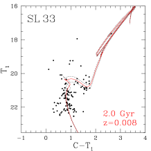
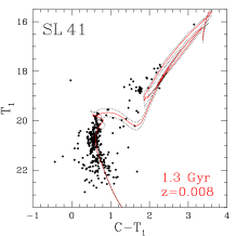
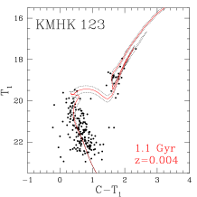
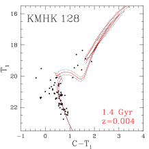
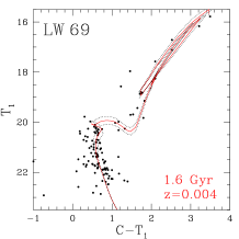
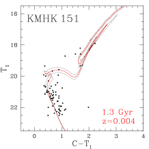
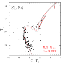
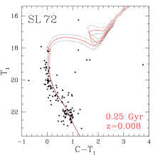
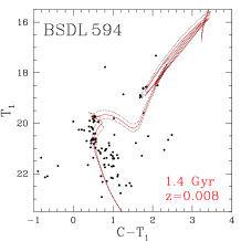
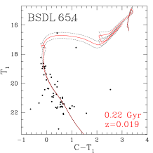
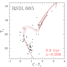
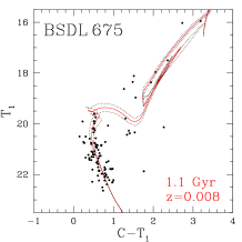
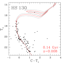
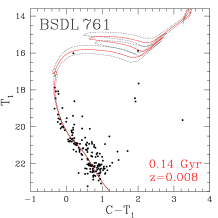
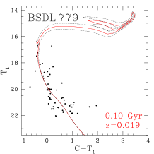
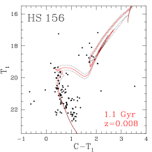
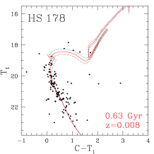
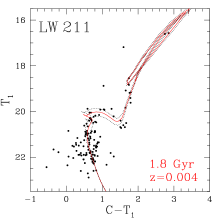
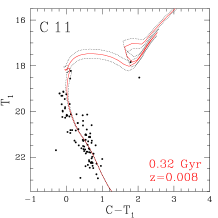
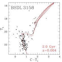
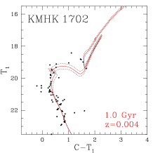
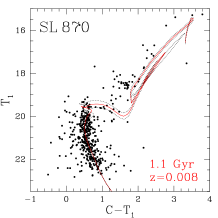
Figure 7: Cleaned Washington ($T_{1},C-T_{1})$ CMDs for the studied clusters. Isochrones from Girardi et al. (2002), computed taking into account overshooting, are overplotted. The red solid and black dashed lines correspond to the derived cluster age and to the ages of the nearest younger and older isochrones.

A second method to derive cluster ages is based on the $\delta(T_{1})$ parameter, defined as the difference in $T_{1}$ magnitude between the RGC and the MSTO in the Washington $(T_{1},C-T_{1})$ CMD. The age is obtained from the following equation given in Geisler et al. (1997):

$$Age(Gyr)=0.23+2.31\times\delta T_{1}-1.80\times{\delta T_{1}}^{2}+0.645\times{\delta T_{1}}^{3},$$ (3)

with a typical error of $\pm$0.3 Gyr. Age determination via $\delta T_{1}$, however, is applicable only to intermediate-age (IACs) and/or old clusters, i.e. generally older than 1 Gyr. Although some clusters seemed to be IACs (1-3 Gyr), it was not possible to determine their ages from $\delta T_{1}$ because the RGC in their CMDs was not clearly detected. This is because sometimes the central regions of the clusters appear to be saturated, perhaps there are just very few RC stars in some faint clusters, or else they are not photometrically well resolved in our images. In these cases, the red giant stars are missed and no clump is visible in the CMDs. This is why we derived ages of only ten clusters older than 1 Gyr based on the $\delta T_{1}$ parameter. The mean $\delta T_{1}$ values were estimated from the average of independent measurements made by two authors. These measurements agreed in general very well. The resulting $\delta T_{1}$ values and the corresponding cluster ages are listed in columns (4) and (5) of Table LABEL:t:results. As can be seen, $\delta T_{1}$ ages agree well with those estimated from the isochrone fitting, which confirms that both procedures allow us to estimate ages on a similar scale.

Pandey et al. (2010) studied the integrated magnitudes and colours for some LMC clusters from synthetic models, among which are BSDL 654, BSDL 675, and BSDL 779. They report ages of 0.16 and 1 Gyr for BSDL 654 and BSDL 675, respectively. These age estimates agree well with ours within the errors (see Table LABEL:t:results). For BSDL 779, however, these authors reported an age of 0.03 Gyr, i.e., substantially younger than the one obtained here. On the other hand, two clusters from our sample, SL 870 and SL 41, were classified in Bica et al. (1996) as belonging to SWB V type (Searle et al. 1980), based on their integrated (B-V) and (U-B) colours. This SWB V type is compatible with clusters belonging to the 0.8-2.0 Gyr range, which agrees well with the age values derived here for these two clusters.

Metallicities for only the two oldest clusters of our sample (SL 33 and BSDL 3158) were also obtained using the [$M_{T_{1}},(C-T_{1})_{0}$] plane with the standard giant branches (SGBs) of Geisler & Sarajedini (1999). As these authors claim, this method should be applied only to star clusters aged 2 Gyr or older. Geisler and Sarajedini demonstrated that the metallicity sensitivity of the SGBs (each giant branch corresponds to an isoabundance curve) is three times higher than that of the V, I technique (Da Costa & Armandroff 1990) and that, consequently, it is possible to determine metallicities three times more precisely for a given photometric error. We followed the SGB procedure of inserting absolute $M_{T_{1}}$ magnitudes and intrinsic $(C-T_{1})_{0}$ colours for the clusters into Fig. 4 of Geisler & Sarajedini (1999) to roughly derive their metal abundances ([Fe/H]) by interpolation (Fig. 8). The derived metallicities were corrected for age effects following the prescriptions given in Geisler et al. (2003). The final age-corrected metallicities for SL 33 and BSDL 3158 are listed in column (8) of Table LABEL:t:results. They agree very well with the Z values associated with the isochrones that best resemble the cluster features. The Girardi et al. (2002) models are computed for [Fe/H] = -1.3 and -0.7 dex, but not for intermediate-metallicity values. We finally adopted for our cluster sample averaged values of the ages and metallicities derived from the two different procedures.

Figure 8: Washington $M_{T_{1}}$ vs. $(C-T_{1})_{0}$ diagram of upper RGB stars in two LMC star clusters, with SGBs taken from Geisler & Sarajedini (1999) superimposed. An age-dependent correction to the indicated metallicities was applied for these clusters.

Table 4: Fundamental parameters of LMC clusters

Name	Deprojected	$E(B-V)$	$\delta T_{1}$	$\delta T_{1}$ Age	Isochrone Age	[Fe/H]isochrone	[Fe/H]SGB
	Distance (∘)			(Gyr)	(Gyr)
SL 33	5.1	0.12	–	–	2.0 $\pm$ 0.2	-0.4	-0.6
SL 41	5.1	0.12	1.0	1.4 $\pm$ 0.4	1.3 $\pm$ 0.1	-0.4	–
KMHK 123	5.0	0.12	–	–	1.1 $\pm$ 0.1	-0.7	–
KMHK 128	5.4	0.11	–	–	1.4 $\pm$ 0.2	-0.7	–
LW 69	4.6	0.12	1.4	1.7 $\pm$ 0.4	1.6 $\pm$ 0.2	-0.7	–
KMHK 151	5.1	0.12	1.1	1.4 $\pm$ 0.4	1.3 $\pm$ 0.1	-0.7	–
SL 54	4.9	0.12	–	–	0.9 $\pm$ 0.1	-0.4	–
SL 73	4.7	0.12	1.3	1.6 $\pm$ 0.4	1.6 $\pm$ 0.2	-0.7	–
SL 72	4.4	0.13	–	–	0.25 $\pm$ 0.03	-0.4	–
BSDL 594	3.4	0.05	0.8	1.3 $\pm$ 0.4	1.4 $\pm$ 0.2	-0.4	–
BSDL 654	3.6	0.03	–	–	0.22 $\pm$ 0.03	0.0	–
BSDL 665	3.6	0.03	–	–	0.9 $\pm$ 0.1	-0.4	–
BSDL 675	3.0	0.06	1.0	1.4 $\pm$ 0.4	1.1 $\pm$ 0.1	-0.4	–
HS 130	2.5	0.06	–	–	0.14 $\pm$ 0.02	-0.4	–
BSDL 761	3.6	0.04	–	–	0.14 $\pm$ 0.02	-0.4	–
BSDL 779	3.3	0.04	–	–	0.10 $\pm$ 0.01	0.0	–
HS 156	2.5	0.06	0.9	1.3 $\pm$ 0.4	1.1 $\pm$ 0.1	-0.4	–
HS 178	3.5	0.04	–	–	0.63 $\pm$ 0.07	-0.4	–
LW 211	4.7	0.10	–	–	1.8 $\pm$ 0.2	-0.7	–
C11	3.4	0.10	–	–	0.32 $\pm$ 0.05	-0.4	–
BSDL 3158	3.5	0.10	1.7	2.1 $\pm$ 0.4	2.0 $\pm$ 0.2	-0.7	-0.8
KMHK 1702	5.3	0.11	0.7	1.2 $\pm$ 0.4	1.0 $\pm$ 0.1	-0.7	–
SL 870	5.4	0.09	0.7	1.2 $\pm$ 0.4	1.1 $\pm$ 0.1	-0.4	–

5 Discussion

The present sample includes 23 mostly unstudied LMC clusters within the narrow age range of 0.1 - 2.1 Gyr, with metallicities between 0.0 and -0.8 dex. To search for possible variations of ages and metallicities as a function of cluster position in the LMC, we calculated deprojected angular distances for our sample using equation (1) of Clariá et al. (2005), assuming that all clusters are part of the LMC inclined disc. We adopted i $\approx$ 35.8^∘ and p’ = 145^∘ for the tilt of the LMC plane and the position angle of the line of nodes, respectively (Olsen & Salyk 2002). The resulting deprojected angular distances are listed in column (2) of Table LABEL:t:results.

Fig. 9 shows that in the comparatively small range of deprojected angular distances considered here (2.5^∘ - 6^∘), the most metal-rich clusters of our sample (filled symbols) tend to lie closer to NGC 1928, whose position was adopted as the LMC centre ($\alpha_{2000}$ = 5^h20^m57^s, $\delta_{2000}$ = -69^∘28’41”). Filled symbols of Fig. 10 show how our derived cluster ages vary as a function of the deprojected distances. As the clusters become older, their corresponding deprojected distances tend to be proportionally larger, thus supporting previous results in similar ranges of deprojected angular distances for clusters (e.g., Piatti et al. 2009) and field stars (Piatti & Geisler 2012).

To examine what the above mentioned position-age-metallicity relationships are like when the range of deprojected angular distances is enlarged, we searched in the literature for previous LMC cluster studies in which ages and metallicities were determined on a similar scale as that of the present cluster sample. We found a total of 76 LMC star clusters with ages and metallicities derived from the Washington $C,T_{1}$ technique using CTIO telescopes and applying the same methods as in the current study (Table A sample of relatively unstudied star clusters in the Large Magellanic Cloud: fundamental parameters determined from Washington photometry). Our 23 clusters increase the current total amount of LMC clusters using Washington photometry by $\sim$ 30%. We calculated deprojected distances for these additional 76 clusters and included them in column (2) of Table A sample of relatively unstudied star clusters in the Large Magellanic Cloud: fundamental parameters determined from Washington photometry. We plot in Figs. 9 and 10 their ages and metallicities as a function of their deprojected distances for three metallicity intervals, [Fe/H] $>$ -0.4 (triangles), -0.4 $\geq$ [Fe/H] $>$ -0.7 (squares), and [Fe/H]  $\leq$ -0.7. When the new 76 clusters are added, the range of deprojected distances increases by a factor of $\sim$ 2.5. Fig. 9 now reveals that although the most metal-rich clusters tend to be located closer to the galaxy centre, clusters with [Fe/H] $<$ -0.4 appear to be distributed over the entire LMC disc, with a high dispersion. This fact reinforces the idea of the nonexistence of a radial metallicity gradient in the LMC, as suggested in several previous studies (e.g., Grocholski et al. 2006; Carrera et al. 2008; Piatti et al. 2009). Fig. 10 includes clusters younger than 3.2 Gyr, since ESO 121-03 ($\sim$ 8.5 Gyr) has not been plotted. As expected, the most metal-poor clusters turn out to be also the older ones. Moreover, cluster formation seems to be concentrated in the inner LMC disc, since younger clusters were formed closer to the LMC centre than the older ones.

Figure 9: Metallicities as a function of deprojected angular distances from the LMC centre for the 23 studied clusters (filled symbols). Clusters included in Table A sample of relatively unstudied star clusters in the Large Magellanic Cloud: fundamental parameters determined from Washington photometry are represented by open symbols. Triangles, squares, and pentagons correspond to the following [Fe/H] intervals: [Fe/H] $>$ -0.4; -0.4 $\geq$ [Fe/H] $>$ -0.7, and [Fe/H] $\leq$ -0.7, respectively. The old cluster ESO 121-03 has not been plotted.

Figure 10: Ages as a function of deprojected angular distances from the LMC centre for the 23 studied clusters (filled symbols). Clusters included in Table 5 are represented by open symbols. Triangles, squares, and pentagons correspond to the following [Fe/H] intervals: [[Fe/H] $>$ -0.4; -0.4 $\geq$ [Fe/H] $>$ -0.7, and [Fe/H] $\leq$ -0.7, respectively. The old cluster ESO 121-03 has not been plotted.

6 Summary and conclusions

We continued the systematic study of star clusters of the LMC carried out using the Washington photometric system. We presented $(T_{1},C-T_{1})$ CMDs for 23 star clusters that lie within the inner disc and outer regions of the LMC. Only five of these clusters have previous age estimates in the literature. However, no metallicity estimate whatsoever has been found for any cluster of our sample. Ages and metallicities were determined by two different methods. We compared the CMDs with theoretical isochrones in the Washington system and also estimated ages using the magnitude difference between the RGC and the MSTO, and derived metallicities by comparing the giant branches with standard calibrating clusters. The two methods applied for determining ages and metallicities agree well with each other. Fourteen clusters are found to be IACs (1-3 Gyr), with [Fe/H] values ranging from -0.4 to -0.7. The remaining nine objects are younger than 1 Gyr, with metallicities between 0.0 and -0.4. By combining the current results with those of a sample of 76 additional clusters with ages and metallicities derived on a scale similar to that of the present work, we confirmed previous findings regarding the chemical evolution of the LMC. We found no evidence of a metallicity gradient and also found that the younger clusters were formed closer to the LMC centre than the older ones.

[x]lcccc Ages and metallicities of LMC star clusters derived from Washington photometry .
Cluster name Deprojected Age (Gyr) [Fe/H] Reference
distance (^∘)
continued.
Cluster name Deprojected Age (Gyr) [Fe/H] Reference
distance (^∘)
SL 8 4.2 1.6 / 1.8 -0.5 1,2
NGC 1697 3.5 0.7$\pm$0.1 0.0 3
HS 38 4.0 0.4$\pm$0.1 -0.4 4
KMHK 229 2.6 1.0$\pm$0.2 -0.4 4
H88-26 3.3 0.8$\pm$0.2 -0.4 4
H88-40 3.5 0.7$\pm$0.2 -0.4 4
SL 126 8.9 1.9 / 2.2 -0.45 1,2
SL 133 5.9 2.2$\pm$0.3 -0.7 3
H88-55 3.3 0.5$\pm$0.1 -0.4 4
SL 154 3.0 0.5$\pm$0.1 -0.4 4
KMHK 506 2.2 0.6$\pm$0.1 -0.4 4
SL 218 2.0 0.05$\pm$0.01 -0.4 5
NGC 1836 1.9 0.4$\pm$0.1 0.0 6
BRHT 4b 1.9 0.10$\pm$0.02 -0.4 5
NGC 1839 1.9 0.12$\pm$0.02 -0.4 5
NGC 1838 2.0 0.10$\pm$0.02 -0.4 5
SL 229 2.1 0.3$\pm$0.1 -0.4 4
SL 244 1.8 1.6 / 1.4$\pm$0.3 -0.7 1,8
BSDL 716 2.2 0.4$\pm$0.1 -0.4 4
SL 262 8.6 2.1 -0.55 1,2
HS 151 1.8 0.8$\pm$0.2 -0.4 4
NGC 1860 1.4 0.25$\pm$0.5 0.0 6
H88-188 2.7 0.5$\pm$0.1 -0.4 4
HS 154 2.5 0.5$\pm$0.1 -0.4 4
SL 293 2.5 0.4$\pm$0.1 -0.4 4
NGC 1863 1.4 0.04$\pm$0.01 -0.4 5
SL 300 2.6 0.4$\pm$0.1 -0.4 4
NGC 1865 1.3 0.9 / 0.5$\pm$0.1 -0.2 1,6
BSDL 1024 1.0 0.16$\pm$0.03 -0.4 4
BSDL 1035 1.2 0.5$\pm$0.1 -0.4 4
H88-245 0.7 0.16$\pm$0.04 -0.4 4
SL 351 1.1 0.5$\pm$0.1 -0.4 4
SL 359 1.3 1.8$\pm$0.3 -0.4 1,8
SL 388 7.0 2.6 / 2.2 -0.65 1,2
IC 2134 6.9 1.0 — 2
SL 451 7.0 2.2 -0.7 1,2
SL 446A 2.0 2.3$\pm$0.3 -0.8 1,8
SL 444 2.0 0.5$\pm$0.1 -0.4 6
SL 490 4.8 1.3$\pm$0.3 -0.4 7
SL 505 2.5 1.6 / 1.2$\pm$0.3 -0.6 1,8
SL 510 1.4 0.13$\pm$0.03 -0.4 4
SL 509 6.6 1.4 / 1.2 -0.85 1,2
LW 224 3.0 0.7$\pm$0.1 0.0 6
LW 231 6.7 0.8$\pm$0.3 -0.4 7
NGC 1997 7.1 2.6$\pm$0.5 -0.7 3
SL 548 3.0 0.4$\pm$0.1 0.0 6
SL 555 3.1 1.6 / 1.7$\pm$0.3 -0.7 1,8
SL 549 5.9 1.3 / 2.0$\pm$0.3 -0.9 1,8
KMHK 1045 1.9 0.6$\pm$0.1 -0.4 4
KMHK 1055 2.0 1.0$\pm$0.2 -0.4 4
SL 588 1.7 0.4$\pm$0.1 -0.4 4
NGC 2093 2.0 0.25$\pm$0.05 -0.4 4
SL 663 4.8 3.0$\pm$0.8 -0.7 3
SL 674 3.9 2.1 / 2.2$\pm$0.3 -0.9 1,8
SL 678 4.0 1.8$\pm$0.3 -0.8 8
H88-333 2.3 0.4$\pm$0.1 -0.4 4
BSDL 2995 2.4 1.0$\pm$0.2 -0.4 4
H7 3.2 1.4 — 1
SL 769 2.9 1.8 -0.5 2
KMHK 1507 3.5 0.8$\pm$0.3 -0.4 7
SL 775 3.5 0.6$\pm$0.3 -0.4 7
OHSC 28 8.3 2.4$\pm$0.5 -0.7 3
NGC 2161 5.9 1.1$\pm$0.3 -0.7 9
NGC 2153 4.6 1.3 — 1
NGC 2155 5.4 3.2$\pm$0.6 -0.9 10
SL 817 3.6 2.5 / 1.5 -0.5 1,2
ESO 121-03 10.4 8.5 -1.05 1,2
SL 842 8.1 1.9 / 2.2 -0.6 1,2
NGC 2213 4.6 1.5 -0.4 11
SL 862 4.7 1.8 -0.85 1,2
OHSC 33 6.2 1.2 / 1.4 -1.0 1,2
SL 874 4.9 1.5$\pm$0.3 -0.7 9
KMHK 1719 5.1 1.4$\pm$0.3 -0.6 9
LW 469 5.9 0.6$\pm$0.1 -0.4 4
SL 896 6.4 2.3$\pm$0.3 -0.6 10
OHSC 37 9.4 2.1 -0.65 1,2
(1) Geisler et al. (1997); (2) Bica et al. (1998); (3) Piatti et al. (2009); (4) Piatti (2012b); (5) Piatti et al. (2003b); (6) Piatti et al. (2003a); (7) Palma et al. (2011); (8) Geisler et al. (2003); (9) Piatti et al. (2011); (10) Piatti et al. (2002); (11) Geisler (1987).