Physical Limits on Cellular Directional Mechanosensing

Abstract

Many eukaryotic cells are able to perform directional mechanosensing by directly measuring minute spatial differences in the mechanical stress on their membranes. Here, we explore the limits of a single mechanosensitive channel activation using a two-state double-well model for the gating mechanism. We then focus on the physical limits of directional mechanosensing by a single cell having multiple mechanosensors and subjected to a shear flow inducing a nonuniform membrane tension. Our results demonstrate that the accuracy in sensing the mechanostimulus direction not only increases with cell size and exposure to a signal, but also grows for cells with a near-critical membrane prestress. Finally, the existence of a nonlinear threshold effect, fundamentally limiting the cell’s ability to effectively perform directional mechanosensing at a low signal-to-noise ratio, is uncovered.

I Introduction

Cells usually dwell in complex microenvironments and, therefore, are inherently sensitive to a variety of biomechanical stimuli, such as blood flow and organ distensions, which induce mechanical stresses in the membrane and cytoskeleton of cells. Recent studies indicate that mechanical forces have a far greater impact on cell functions than previously appreciated. Eukaryotic cells, such as epithelial cells, amoebae, and neutrophils, are remarkably sensitive to shear flow direction Arnadottir ; ShearFlow ; Park ; Moares .

More quantitatively, endothelial cells have been found to respond to laminar shear stress levels in the range of 0.02–0.16 Pa with a cellular alignment in the direction of the flow for a shear stress beyond 0.5 Pa Olesen ; Davies . In other instances, some eukaryotic cells performed parallel or perpendicular cellular alignment to the shear flow direction Park . Xenopus laevis oocytes were found to respond to laminar shear stress of magnitude 0.073 Pa, whereas, the amoeba Dictyostelium discoideum exhibits shear-flow induced motility in the direction of creeping flows with shear stresses as low as 0.7 Pa Decave . Similar magnitudes of this shear-stress based mechanostimulus for other types of cells are reported in Ref. Orr . To better appreciate the exquisite sensitivity of those cells S&S , it is worth highlighting the minuteness of those mechanostimuli. For instance, a characteristic shear stress of magnitude $\sigma\sim 1$ Pa generates a maximum excess membrane tension $\Delta\gamma_{\textrm{\tiny max}}\sim\sigma R$, which for a typical cell size of $R\sim 10~{}\upmu\textrm{m}$ is on the order of $10~{}\upmu\textrm{N}\cdot\textrm{m}^{-1}$. According to Rawicz et al. Rawicz , such a value represents a minuscule membrane tension. Furthermore, this membrane tension induced by the shear stress is 1 or 2 orders of magnitude smaller than typical lytic resting membrane tensions: $\gamma_{0}\sim 1$–$2~{}\textrm{mN}\cdot\textrm{m}^{-1}$ Opsahl . From the dynamical standpoint, the lower the shear rate, the longer the exposure required for a cell to respond Moares . Finally, mechanosensing has been shown to be of paramount importance to self-organizing behaviors of those social cells Bouffanais .

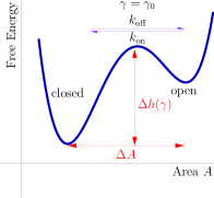
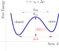
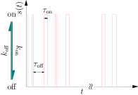
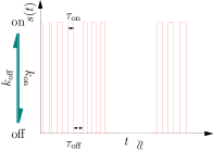
Figure 1: (Color online) Schematic of the two-well model for the MSC gating. (a) Energy profile with prestress $\gamma_{0}$ and (b) with additional prestress $\gamma=\gamma_{0}+\Delta\gamma$ (b); $A$ is the MSC in-plane surface area and $\Delta A$ is its change when opening up; $\Delta h$ is the intrinsic energy barrier in the absence of applied tension, $K_{A}$ is the area stretch modulus of the harmonic profiles, taken identical for both wells. (c) and (d) Associated time series $s(t)$ of the residence periods $\mathcal{T}$ spent in open or closed states.

Mechanosensitive ion channels (MSCs) are present in nearly all cell types Martinac ; they are integral membrane proteins responding over a wide dynamic range to mechanostimuli subsequently transduced into electrochemical signals Arnadottir . There appear to be two modes of action for MSCs: (i) those that receive stress from fibrillar proteins resulting in gating, and (ii) cases in which tension in the surrounding bilayer forces the channel to open. Our focus is on the latter type—the stretch-activated channels—in which the stimulus mechanically deforms the membrane’s lipid bilayer that, in turn, triggers MSC conformational changes through an intricate mechanical coupling Arnadottir ; Ursell . It is important to recall that the high sensitivity of the cellular mechanosensory apparatus does not originate from the MSCs themselves but from an efficient coupling between the channel gating machinery and the cellular structures that transmit the force Orr . The existence of calcium-based stretch-activated MSCs in the amoeba Dictyostelium discoideum has recently been revealed by Lombardi et al. Lombardi , which is believed to be at the root of its shear-flow induced motility Decave improved by calcium mobilization Fache .

MSCs adopt conformational states with distinct functional properties in response to the applied tension along the plane of the cell membrane instead of the normal pressure Gustin ; Sokabe&Sachs ; Sokabe . The gating of these transient receptor channels is to a good approximation represented by a two-state double-well model Ursell ; Sukharev&Corey  [see Figs. 1 and 1]. Directional mechanosensing requires cells to make accurate decisions based on biased stochastic transitions between MSC conformational states [see Figs. 1 and 1]. Although a fundamental bound on the accuracy of directional chemical gradient sensing was derived Endres ; HuSNR , no theory exists for the physical limits of directional mechanosensing.

II Single mechanosensitive ion channel sensing

In this section, our focus is the physical limitations in sampling by a single MSC, subject to a mild shear flow inducing minute changes $\Delta\gamma\ll\gamma_{0}$ to the lateral membrane tension $\gamma=\gamma_{0}+\Delta\gamma$.

II.1 Two-state double-well model for the gating mechanism

We consider a single MSC, which is a specialized transmembrane protein that can undergo a distortion in response to external mechanical forces applied through the lipid bilayer itself. At its simplest, this mechanical deformation can be described as a conformational transition between closed and open states separated by a free energy barrier denoted as $\Delta h$. In the particular case of the gating of the well-studied bacterial large conductance mechanosensitive channel MscL, the energy difference between the closed and the fully open states in the unstressed membrane was found to be $18.6k_{\textrm{\tiny B}}T$ with an associated energy barrier $\Delta h\sim 38k_{\textrm{\tiny B}}T$ Sukharev . Without loss of generality, we assume that both conformational states, open and closed, are symmetrically positioned with respect to the free energy barrier, which implies that the absolute area change between the bottom of each wells is $\Delta A/2$. We account for the elasticity of each state—assumed identical and harmonic for both states—by considering a quadratic dependence of the free energy in the lateral membrane tension $\gamma$ Sukharev&Corey . The unidirectional transition rates, given in Eyring’s form, are

$$k_{\textrm{\scriptsize{on}}} =k_{0}\exp\left(-\frac{\gamma\Delta A/2}{k_{\textrm{\tiny B}}T}-\frac{\gamma^{2}A}{2K_{A}k_{\textrm{\tiny B}}T}\right),$$ (1)

$$k_{\textrm{\scriptsize{off}}} =k_{0}\exp\left(\frac{\gamma\Delta A/2-\Delta h}{k_{\textrm{\tiny B}}T}-\frac{\gamma^{2}A}{2K_{A}k_{\textrm{\tiny B}}T}\right),$$ (2)

where $k_{0}$ is a scaling factor, $A$ is the MSC in-plane surface area, $\Delta A$ is its change in the in-plane area when opening up, $\gamma$ is the lateral membrane tension, and $K_{A}$ is the area stretch modulus. For clarity, we omit the thermal energy $k_{\textrm{\tiny B}}T$ in what follows. We consider, here, a weak mechanostimulus inducing minute changes $\Delta\gamma$ in the membrane tension $\gamma=\gamma_{0}+\Delta\gamma$ with $\Delta\gamma\ll\gamma_{0}$, $\gamma_{0}$ being the cell’s membrane prestress. At the first order in $\Delta\gamma$, the unidirectional transition rates can be expressed as

$$k_{\textrm{\scriptsize{on}}} =k_{0}\exp\left(-\frac{\gamma_{0}\Delta A}{2}-\frac{\gamma_{0}^{2}A}{2K_{A}}\right)\exp\left(-(1+\alpha)\frac{q}{2}\right),$$ (3)

$$k_{\textrm{\scriptsize{off}}} =k_{0}\exp\left(\frac{\gamma_{0}\Delta A}{2}-\Delta h-\frac{\gamma_{0}^{2}A}{2K_{A}}\right)\exp\left((1-\alpha)\frac{q}{2}\right),$$ (4)

where $q=\Delta\gamma\Delta A$ is the extra work generated by the extracellular mechanical signals. The nondimensional parameter $\alpha=2\gamma_{0}A/(K_{A}\Delta A)$ represents the ratio of the total energy $\gamma_{0}\Delta A/2$ expanded for the in-plane deformation of the MSC to the energy $K_{A}(\Delta A/2)^{2}/A$, associated with the membrane thinning due to the membrane volume conversation Ursell . In the particular case of MscL gating, one finds $\alpha\sim 0.58$, given that $\gamma_{0}=3.5k_{\textrm{\tiny B}}T/\textrm{nm}^{2}$, $\Delta A=6\textrm{~{}nm}^{2}$, $A=30\textrm{~{}nm}^{2}$ and $K_{A}=60k_{\textrm{\tiny B}}T/\textrm{nm}^{2}$ Ursell ; Rawicz ; Sukharev .

Such a perturbation $\Delta\gamma$ to the lateral membrane tension induces a stretching of the MSC, triggering its opening if the associated free energy surpasses the barrier $\Delta h$. An internal feedback mechanism is responsible for closing down the MSCs which are relentlessly switching between open and closed states (see Fig. 1). This dynamics is characterized by the binary sequence $s(t)$, spent in both possible states. This process is essentially a Markovian telegraph process: Memoryless transitions are entirely determined by a switching rate Gillespie . Therefore the lengths of open and closed intervals have exponential distributions with means $1/k_{\textrm{\scriptsize{on}}}$ and $1/k_{\textrm{\scriptsize{off}}}$, respectively, $k_{\textrm{\scriptsize{on}}}$ and $k_{\textrm{\scriptsize{off}}}$ being the unidirectional transition rates in conformational states.

II.2 Signal estimation by linear regression

To know how well a cell can determine the shear stress applied to its membrane, it is assumed that information is derived from its MSC states based on the concept of “perfect instrument” registering switching events Berg&Purcell . MSCs switch between open and closed states with $s(t)=1$ for $t\in\mathcal{T}_{\textrm{\scriptsize{on}}}$ and $s(t)=0$ for $t\in\mathcal{T}_{\textrm{\scriptsize{off}}}$. We use the time series $s(t)$—as being the time record of MSC states measured by a perfect instrument—to investigate the dynamics of a given MSC over a long signal exposure time, i.e. for $\mathcal{T}\gg 1/k_{\textrm{\scriptsize{on}}}$ and $\mathcal{T}\gg 1/k_{\textrm{\scriptsize{off}}}$. We perform a linear regression (LR) of the binary time series $s(t)$. In the limit of long time series $\mathcal{T}$, with starting time $t_{0}$, the mean and variance of $s(t)$ over the of observation are classically given by Gillespie ,

$$S =\frac{1}{\mathcal{T}}\int_{t_{0}}^{t_{0}+\mathcal{T}}s(t)\,\text{d}t=\frac{k_{\textrm{\scriptsize{on}}}}{k_{\textrm{\scriptsize{on}}}+k_{\textrm{\scriptsize{off}}}},$$ (5)

$$\sigma_{s}^{2} =\langle(\delta s)^{2}\rangle=\frac{k_{\textrm{\scriptsize{on}}}k_{\textrm{\scriptsize{off}}}}{(k_{\textrm{\scriptsize{on}}}+k_{\textrm{\scriptsize{off}}})^{2}}.$$ (6)

Still, in the limit of long time series,

$$S\simeq\langle s\rangle=\frac{k_{\textrm{\scriptsize{on}}}}{k_{\textrm{\scriptsize{on}}}+k_{\textrm{\scriptsize{off}}}}\bigg{|}_{q=\tilde{q}}=\frac{1}{1+\exp(\tilde{q}-\Delta h_{\textrm{\scriptsize eff}})},$$ (7)

where $\langle s\rangle$ is the ensemble average of $s(t)$, $\tilde{q}$ is the true value of $q$, and $\Delta h_{\textrm{\scriptsize eff}}=\Delta h-\gamma_{0}\Delta A$ is the effective free energy barrier reduced by the existing prestress action. The signal can be inferred from the fraction of MSC active time $S$ with $S\simeq\langle s\rangle$ for long $\mathcal{T}$. To compute the variance of $S$, the covariance of $s(t)$ is needed, and it can be calculated directly from its definition,

$$G(t,t^{\prime})\equiv\langle s(t)s(t^{\prime})\rangle-{\langle s(t)\rangle}^{2} =\sigma_{s}^{2}e^{-|t-t^{\prime}|/\tau},$$

$$=\sigma_{s}^{2}e^{-|t-t^{\prime}|(k_{\textrm{\scriptsize{on}}}+k_{\textrm{\scriptsize{off}}})}.$$ (8)

If we repeat this observation many times, starting at wildly different times $t_{0}$, the variance of $S$ is

$$\sigma_{S}^{2}=\frac{1}{{\cal T}^{2}}\int_{0}^{{\cal T}}\text{d}t\int_{0}^{{\cal T}}\text{d}t^{\prime}G(t,t^{\prime})=\frac{2}{\mathcal{T}}\frac{k_{\textrm{\scriptsize{off}}}k_{\textrm{\scriptsize{on}}}}{(k_{\textrm{\scriptsize{off}}}+k_{\textrm{\scriptsize{on}}})^{3}}.$$ (9)

A standard LR yields

$$\delta q=\frac{k_{\textrm{\scriptsize{on}}}}{k_{\textrm{\scriptsize{off}}}}\delta\left(\frac{S}{1-S}\right)=\frac{k_{\textrm{\scriptsize{on}}}}{k_{\textrm{\scriptsize{off}}}}\frac{\delta S}{S^{2}},$$ (10)

and the following estimate for $q=\Delta\gamma\Delta A$:

$$q^{\rm LR}=\Delta h_{\textrm{\scriptsize eff}}+\ln\frac{S}{1-S}=\Delta h_{\textrm{\scriptsize eff}}+\ln\frac{\mathcal{T}_{\textrm{\scriptsize{on}}}}{\mathcal{T}_{\textrm{\scriptsize{off}}}},$$ (11)

where $\Delta h_{\textrm{\scriptsize eff}}$=$\Delta h-\gamma_{0}\Delta A$ is the effective energy barrier, reduced by the existing membrane prestress $\gamma_{0}$. From Eqs. (10) and (11), we obtain the associated variance,

$$\sigma_{q}^{2}=\frac{k_{\textrm{\scriptsize{on}}}^{2}}{k_{\textrm{\scriptsize{off}}}^{2}}\frac{\sigma_{S}^{2}}{S^{4}}=\frac{2(k_{\textrm{\scriptsize{on}}}+k_{\textrm{\scriptsize{off}}})}{\mathcal{T}(k_{\textrm{\scriptsize{on}}}k_{\textrm{\scriptsize{off}}})}=\frac{2}{n},$$ (12)

in terms of the number of registered switches $n$ defined as

$$n\equiv\mathcal{T}\frac{k_{\textrm{\scriptsize{on}}}k_{\textrm{\scriptsize{off}}}}{k_{\textrm{\scriptsize{on}}}+k_{\textrm{\scriptsize{off}}}},$$ (13)

and physically representing the number of transitions between the two conformational states. Note that if $k_{\textrm{\scriptsize{on}}}\ll k_{\textrm{\scriptsize{off}}}$ or $k_{\textrm{\scriptsize{on}}}\gg k_{\textrm{\scriptsize{off}}}$, $n$ can simply be expressed as $n\simeq\mathcal{T}/\textrm{max}(k_{\textrm{\scriptsize{on}}}^{-1},k_{\textrm{\scriptsize{off}}}^{-1})$.

II.3 Signal estimation using a maximum likelihood estimator

It is still unclear how exactly a cell performs its signal estimation based on the register of switching events. The LR presented in the previous section appears as the most rudimentary form of statistical estimation. Alternatively, a maximum likelihood estimate (MLE) Kay can be sought for the two-state discrete-valued telegraph process which is generated by switching values at jump times of a Poisson process Gillespie .

For a long exposure to a signal—i.e., for large $\mathcal{T}=\mathcal{T}_{\textrm{\scriptsize{on}}}+\mathcal{T}_{\textrm{\scriptsize{off}}}$— and given the unidirectional transition rates $k_{\textrm{\scriptsize{on}}}$ and $k_{\textrm{\scriptsize{off}}}$, the likelihood function is obtained by acknowledging the fact that we are in the presence of a stationary Poisson process,

$$\mathcal{L}=\frac{(k_{\textrm{\scriptsize{on}}}\mathcal{T}_{\textrm{\scriptsize{on}}})^{n}}{n!}e^{-k_{\textrm{\scriptsize{on}}}\mathcal{T}_{\textrm{\scriptsize{on}}}}\cdot\frac{(k_{\textrm{\scriptsize{off}}}\mathcal{T}_{\textrm{\scriptsize{off}}})^{n}}{n!}e^{-k_{\textrm{\scriptsize{off}}}\mathcal{T}_{\textrm{\scriptsize{off}}}},$$ (14)

where $\mathcal{T}_{\textrm{\scriptsize{on}}}$ (respectively, $\mathcal{T}_{\textrm{\scriptsize{off}}}$) is the total open (respectively, closed) time and $n$ is the number of switching events. When omitting the unessential constant terms, the log-likelihood function is cast as

$$\ln\mathcal{L}=-(k_{\textrm{\scriptsize{on}}}\mathcal{T}_{\textrm{\scriptsize{on}}}+k_{\textrm{\scriptsize{off}}}\mathcal{T}_{\textrm{\scriptsize{off}}})+n\ln(k_{\textrm{\scriptsize{off}}}k_{\textrm{\scriptsize{on}}}).$$ (15)

The MLE is considered to provide an estimate of $q$. To this aim, maxima of the first-order derivative of the above log-likelihood are sought

$$\left(\frac{\partial\ln\mathcal{L}}{\partial q}\right)(q=\hat{q}_{\textrm{\tiny{MLE}}}) =-k_{\textrm{\scriptsize{on}}}\mathcal{T}_{\textrm{\scriptsize{on}}}(1+\alpha)$$

$$- k_{\textrm{\scriptsize{off}}}\mathcal{T}_{\textrm{\scriptsize{off}}}(1-\alpha)+2n\alpha=0,$$ (16)

which yields

$$\hat{q}_{\textrm{\tiny{MLE}}}=\Delta h_{\textrm{\scriptsize eff}}+\ln\frac{\mathcal{T}_{\textrm{\scriptsize{on}}}}{\mathcal{T}_{\textrm{\scriptsize{off}}}}.$$ (17)

To quantify the uncertainty associated with the above maximum likelihood estimation, one has to consider the second-order derivative of the log-likelihood function,

$$\frac{\partial^{2}\ln{\cal L}}{\partial q^{2}}=-k_{\textrm{\scriptsize{on}}}\mathcal{T}_{\textrm{\scriptsize{on}}}(1+\alpha)^{2}-k_{\textrm{\scriptsize{off}}}\mathcal{T}_{\textrm{\scriptsize{off}}}(1-\alpha)^{2}$$ (18)

to ascertain the normalized variance in the long exposure to the signal limit,

$$\sigma_{q}^{2}=-\left<\left(\frac{\partial^{2}\ln\mathcal{L}}{\partial q^{2}}\right)(q=\hat{q}_{\textrm{\tiny{MLE}}})\right>^{-1}=\frac{2}{(1+\alpha^{2})n}.$$ (19)

According to the Cramér-Rao lower bound (CRLB), the variance $\sigma_{q}^{2}$ sets the lowest measurement uncertainty through sampling Kay .

The uncertainties of mechanosensing using LR and MLE [Eqs. (12) and (19)] show that for a given stimulus exposure, statistical fluctuations limit the precision with which a single MSC can determine the stimulus amplitude. Similar to chemosensing, MLE yields a more accurate mechanosensing lower limit than LR Endres , albeit for fundamentally different reasons. Indeed, the two estimates for $q$ given by the LR and the MLE are identical, whereas, the associated variances are different. In this particular problem, the linear regression is intrinsically limited by its linear character and only captures the lowest-order term which does not involve $\alpha$. This is, of course, no longer the case with the MLE. From a physical standpoint, it is like the LR is not able to account for the thinning effects of the lipid bilayer; the variations in the thickness of the lipid bilayer are negligible for high values of $K_{A}$, i.e. for near-zero values of $\alpha$. The very presence of $\alpha=2\gamma_{0}A/(K_{A}\Delta A)$ in Eq. (19) highlights the connection between the mechanical properties of the cell and the measurement uncertainty zeroalpha .

III Limits of cellular mechanosensing

In this section, our focus is the physical limitations in sampling by an array of MSCs distributed across the cell, subject to a mild shear flow inducing nonuniform minute changes $\Delta\gamma\ll\gamma_{0}$ to the lateral membrane tension $\gamma=\gamma_{0}+\Delta\gamma$.

III.1 Model of a cell subjected to a linear shear flow

We now turn to directional mechanosensing by an entire cell, focusing on the idealized case of $N$ uniformly distributed MSCs on the equator (only) of a spherical cell of radius $R$. Observing the MSC distribution is experimentally challenging, but it is very unlikely that it is homogeneous. For the sake of analytical simplicity, our model does not consider this fact. We assume the MSCs to be independent, neglecting inter-MSC interactions. One might argue that local interactions among the MSCs could result globally in a cooperative effect which may help smaller cells better discriminate the signal direction—see Ref. Duke regarding the cooperativity between chemical receptors for chemotactic E. coli. The present analysis would, thus, provide conservative estimates for this problem.

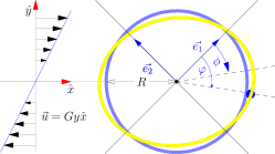
Figure 2: (Color online) Cell deformation under a linear shear flow with shear rate $G$. The elliptic curve represents the intersection of the ellipsoid with the $xy$ plane. The circular curve is the initial membrane, and $\vec{e}_{1}$ is the direction of the largest elongation rate eigenvector Marmottant ; the dot represents a given MSC.

Fluid shear stress, which occurs naturally in a variety of physiological conditions, is one of the most important mechanostimuli Arnadottir ; ShearFlow ; Park ; Moares . Furthermore, cell locomotion generates Stokes flows which can be sensed by neighboring cells Bouffanais ; Moares . Specifically, fluid shear stress induces a nonuniform tension on the cell’s lipid bilayer triggering an asymmetric stretch activation of some MSCs, themselves giving rise to an intracellular biochemical cascade driving pseudopod extensions preferentially in the direction of the tension gradient ShearFlow . At the cell’s microscale, any natural flow field approximates locally to a linear shear flow (see Fig. 2). For an artificial spherical cell (vesicle) subject to small deformations due to a weak mechanical stimulus, the tension distribution at the equator (see Fig. 2) reads Marmottant

$$\gamma(\varphi) =\gamma_{0}+\Delta\gamma(\varphi),$$ (20)

$$\Delta\gamma =-\frac{5}{4}\eta GR\cos 2(\varphi-\phi),$$ (21)

$\eta$ being the viscosity and $\phi$ being the phase angle difference between the minimum tension point and the largest elongation axis Marmottant . An MSC located in a high-tension zone has a higher probability to open up. This spatial asymmetry creates an angular bias in the fluctuations of the $N$ time traces $\mathbf{S}=\{S_{1},\ldots,S_{N}\}$ across the cell, $S_{i}$ being the fraction of open state of the $i$th MSC at location $\varphi=\varphi_{i}$. We prove that, by a global statistical processing of $\mathbf{S}$, a cell can infer the stimulus direction. The uncertainty due to the ubiquitous and limiting presence of noise is also derived.

III.2 Statistics for the shear-stress induced signal at the cellular level

When exposing a cell to shear stress [see Fig. 2 and Eq. (20)], the nonuniform perturbation in its membrane tension $\Delta\gamma$ induces an uneven MSC redistribution across the cell. Using the white-noise approximation, the conformational state of the $i$-th MSC at $\varphi_{i}$, subject to $q_{i}=\Delta\gamma(\varphi_{i})\Delta A=-Q\cos 2(\varphi_{i}-\phi)$ with $Q=\frac{5}{4}\eta GR\Delta A$, is $S_{i}=\langle S_{i}\rangle+\eta_{i}$ with

$$\langle S_{i}\rangle=\frac{k_{\textrm{\scriptsize{on}}}^{i}}{k_{\textrm{\scriptsize{on}}}^{i}+k_{\textrm{\scriptsize{off}}}^{i}}=\frac{1}{1+\exp(-\Delta h_{\textrm{\scriptsize eff}}-Q\cos 2(\varphi_{i}-\phi)),}$$ (22)

and

$$\langle\eta_{i}\eta_{j}\rangle=\frac{2}{\mathcal{T}}\frac{k_{\textrm{\scriptsize{off}}}^{i}k_{\textrm{\scriptsize{on}}}^{i}}{(k_{\textrm{\scriptsize{off}}}^{i}+k_{\textrm{\scriptsize{on}}}^{i})^{3}}\delta_{ij}=\sigma_{S_{i}}^{2}\delta_{ij},$$ (23)

where $\sigma_{S_{i}}^{2}$ takes the form of Eq. (9) at the $i$th location. The MSC signal $\mathbf{S}$ is a vector of independent Gaussian random variables with different means but approximately identical variances $\sigma_{S}^{2}$. From Eq. (9), we find that $\sigma_{S}^{2}$ decreases as $\mathcal{T}$ increases, with $\sigma_{S}^{2}\rightarrow 0$ in the limit of $\mathcal{T}\rightarrow\infty$. Instead of time averaging over long exposure to signal time $\mathcal{T}$, we consider ensemble averaging over $m$ independent MSCs subject to the same signal, thus giving $S=\frac{1}{m}\sum_{k=1}^{m}s_{k}$. The variance associated with this ensemble averaging is

$$\sigma_{S}^{2}=\frac{1}{m}\frac{k_{\textrm{\scriptsize{on}}}k_{\textrm{\scriptsize{off}}}}{(k_{\textrm{\scriptsize{on}}}+k_{\textrm{\scriptsize{off}}})^{2}}.$$ (24)

From Eqs. (9) and (24), one can establish that a single MSC observed over time $\mathcal{T}$ is statistically equivalent to ensemble averaging over $m\equiv\frac{1}{2}\mathcal{T}(k_{\textrm{\scriptsize{on}}}+k_{\textrm{\scriptsize{off}}})=\frac{\mathcal{T}}{2\tau}$ independent MSCs. This allows us to recast the white Gaussian noise component as

$$\langle\eta_{i}\eta_{j}\rangle=\frac{1}{m}\frac{k_{\textrm{\scriptsize{off}}}^{i}k_{\textrm{\scriptsize{on}}}^{i}}{(k_{\textrm{\scriptsize{off}}}^{i}+k_{\textrm{\scriptsize{on}}}^{i})^{2}}\delta_{ij}.$$ (25)

As we are working in the limit of small membrane deformations induced by a mild mechanical stimulus, we expand $\langle S_{i}\rangle$ in small $Q=\frac{5}{4}\eta GR\Delta A$ up to the leading order

$$\langle S_{i}\rangle \simeq\langle S\rangle-\mu\cos 2(\varphi_{i}-\phi),$$ (26)

with

$$\langle S\rangle =\frac{k_{\textrm{\scriptsize{on}}}}{k_{\textrm{\scriptsize{on}}}+k_{\textrm{\scriptsize{off}}}}\bigg{|}_{Q=0},$$ (27)

and where $\mu=m\sigma_{S}^{2}Q$ is the signal amplitude. At the first order in $Q$ for $S_{i}$, we also have

$$\langle\eta_{i}\eta_{j}\rangle\simeq\frac{1}{m}\frac{k_{\textrm{\scriptsize{off}}}k_{\textrm{\scriptsize{on}}}}{(k_{\textrm{\scriptsize{off}}}+k_{\textrm{\scriptsize{on}}})^{2}}\bigg{|}_{Q=0}\delta_{ij}=\sigma_{S}^{2}(Q=0)\delta_{ij}.$$ (28)

To summarize, at the leading order in $Q$,

$$S_{i}\approx\langle S\rangle-m\sigma_{S}^{2}Q\cos 2(\varphi_{i}-\phi)+\eta_{i},$$ (29)

where $\{\langle S\rangle,\sigma_{S}^{2}\}=\left\{\frac{k_{\textrm{\scriptsize{on}}}}{k_{\textrm{\scriptsize{on}}}+k_{\textrm{\scriptsize{off}}}},\frac{k_{\textrm{\scriptsize{on}}}k_{\textrm{\scriptsize{off}}}}{m(k_{\textrm{\scriptsize{on}}}+k_{\textrm{\scriptsize{off}}})^{2}}\right\}_{|Q=0}$. The associated signal-to-noise ratio (SNR) Kay is

$$\kappa\equiv\frac{\mu^{2}}{\sigma_{S}^{2}}=m^{2}{\sigma_{S}^{2}}Q^{2}.$$ (30)

III.3 Maximum likelihood estimation of the magnitude and direction of the mechanostimulus

The signal (29) has a classical form—sinusoidal in phase with added white Gaussian noise—commonly encountered in signal processing applications Kay . Estimating the shear-flow direction for the cell is strictly equivalent to estimating the phase $\phi$ of (29). Given the nonlinear nature of the relationship between the mechanostimulus and the spatiotemporal signal available to the cell, a nonlinear statistical estimation is required. A nonlinear MLE of $\mathbf{\Theta}=\{Q,\phi\}$ can be achieved by resorting to the jointly sufficient statistics Kay given by:

$$z_{1} =\sum_{i=1}^{N}(S_{i}-\langle S\rangle)\cos 2\varphi_{i},$$ (31)

$$z_{2} =\sum_{i=1}^{N}(S_{i}-\langle S\rangle)\sin 2\varphi_{i}.$$ (32)

The associated joint probability density function reads

$$p(\mathbf{Z})=\frac{2}{\pi\sigma_{S}^{2}N}\exp \left(-\frac{N\mu^{2}}{4\sigma_{S}^{2}}+\frac{\mu}{\sigma_{S}^{2}}(z_{1}\cos 2\phi-z_{2}\sin 2\phi)\right)$$

$$\times \exp\left(-\frac{1}{N\sigma_{S}^{2}}(z_{1}^{2}+z_{2}^{2})\right),$$ (33)

leading to the following expression:

$$p(\mathbf{Z})=\frac{2e^{-N\kappa/4}}{\pi\sigma_{S}^{2}N}\exp\left[\frac{\mu(z_{1}\cos 2\phi-z_{2}\sin 2\phi)}{\sigma_{S}^{2}}-\frac{z_{1}^{2}+z_{2}^{2}}{N\sigma_{S}^{2}}\right].$$ (34)

Thus, the likelihood function, $\mathcal{L}=p(\mathbf{Z}|\mathbf{\Theta})$, is given by the joint probability density function which gives access to the log-likelihood

$$\ln\mathcal{L} =-\frac{N\mu^{2}}{4\sigma_{S}^{2}}+\frac{\mu}{\sigma_{S}^{2}}(z_{1}\cos 2\phi-z_{2}\sin 2\phi)-\frac{1}{N\sigma_{S}^{2}}(z_{1}^{2}+z_{2}^{2}),$$

$$=mQ(z_{1}\cos 2\phi-z_{2}\sin 2\phi)-\frac{m^{2}N\sigma_{S}^{2}}{4}Q^{2}.\$$ (35)

The maximum likelihood estimators for the vector parameter $\mathbf{\Theta}=\{Q,\phi\}$ are defined to be the value that maximizes the likelihood function over that allowable domain for $\mathbf{\Theta}$ and it is found from

$$\frac{\partial\ln p(\mathbf{Z}|\mathbf{\Theta})}{\partial Q}(Q=\hat{Q}_{\textrm{\tiny{MLE}}}) =0,$$ (36)

$$\frac{\partial\ln p(\mathbf{Z}|\mathbf{\Theta})}{\partial\phi}(\phi=\hat{\phi}_{\textrm{\tiny{MLE}}}) =0$$ (37)

yielding, respectively,

$$\hat{Q}_{\textrm{\tiny{MLE}}} =\frac{2\sqrt{z_{1}^{2}+z_{2}^{2}}}{Nm\sigma_{S}^{2}},$$ (38)

$$\hat{\phi}_{\textrm{\tiny{MLE}}} =-\frac{1}{2}\arctan\frac{z_{2}}{z_{1}}.$$ (39)

The CRLB yields the respective variances of the MLE, $\hat{\mathbf{\Theta}}_{\textrm{\tiny{MLE}}}=(\hat{Q}_{\textrm{\tiny{MLE}}},\hat{\phi}_{\textrm{\tiny{MLE}}})$, which are calculated by means of the inverse of the Fisher information matrix, which is the negative of the expected value of the Hessian matrix Kay ,

$$\sigma_{\hat{Q}}^{2} =-\left<\frac{\partial^{2}\ln{\cal L}}{\partial Q^{2}}\right>^{-1}=\frac{2}{Nm^{2}\sigma_{S}^{2}},$$ (40)

$$\sigma_{\hat{\phi}}^{2} =-\left<\frac{\partial^{2}\ln{\cal L}}{\partial\phi^{2}}\right>^{-1}=\frac{1}{2Nm^{2}\sigma_{S}^{2}\hat{Q}^{2}}=\frac{1}{2N{\kappa}},$$ (41)

where $\kappa\equiv\mu^{2}/\sigma_{S}^{2}$ is the SNR. Both uncertainties in the signal amplitude and phase are inversely proportional to $m=\frac{\mathcal{T}}{2\tau}$ and $\sqrt{N}$, i.e., favoring longer signal exposure time $\mathcal{T}$ with as many MSCs as possible.

III.4 Analysis of the results

Typically, eukaryotic cells are 10–100 $\,\mathrm{\upmu m}$ across with uniform MSC surface density on the order of $1/\,\mathrm{\upmu m^{2}}$ Morris ; Davies , and the number of MSCs increases with the cell surface area $A$ as $N=N_{0}R^{2}$. Given that $Q\sim R$, we get the paramount fact that the SNR $\kappa$ varies like $R^{4}$; this amounts to an enormous $10^{4}$ ratio in SNRs for small and large eukaryotic cells. Larger cells are considerably more effective at directional mechanosensing. Interestingly, we also find that $\kappa\propto 1/{\sigma_{\hat{\phi}}^{2}}$, exactly like the case of eukaryotic directional gradient chemosensing, despite fundamental differences in signaling mechanisms HuSNR .

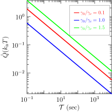
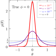
Figure 3: (Color online) (a) Relationship between observation time $\mathcal{T}$ and MLE estimated signal amplitude $\hat{Q}$, for $\gamma_{0}/\gamma_{c}=0.1,\ 1,\ 1.5$; (b) probability density function (PDF) of the phase estimate for a true value $\phi=0$ for different SNR values $\kappa$. The following values are used Ursell ; Sukharev&Corey : $K_{A}=60k_{\textrm{\tiny B}}T/\,\mathrm{nm}^{2}$, $\Delta h=38k_{\textrm{\tiny B}}T$, $A=30\,\mathrm{nm}^{2}$, $\Delta A=10\,\mathrm{nm}^{2}$, $\gamma_{c}=1.0k_{\textrm{\tiny B}}T/\,\mathrm{nm}^{2}$, $1/k_{0}=1\,\mathrm{ms}$, and $N=200$.

Understanding how the SNR relates to cell characteristics—specifically elastic and gating properties—allows one to uncover some essential features of eukaryotic directional mechanosensing. For a given $\mathcal{T}$, the SNR reads

$$\kappa=n\hat{Q}^{2}=\left[\frac{k_{0}\mathcal{T}}{2}\frac{\exp(-\gamma_{0}^{2}A/(2K_{A})-\gamma_{0}\Delta A/2)}{1+\exp(\Delta h-\gamma_{0}\Delta A)}\right]\hat{Q}^{2},$$ (42)

$n$ being the number of switching events. Considering varying prestresses $\gamma_{0}$ in Eq. (42), one finds that $\kappa$ achieves large values about its maximum attained at the critical prestress $\gamma_{c}=\Delta h/\Delta A$ such that $\Delta h_{\textrm{\scriptsize eff}}=0$. At this point, it is worth highlighting that the cortical cytoskeleton structurally supports the fluid bilayer, thus, providing the cell membrane with a shear rigidity that is lacking in simple bilayer vesicles Hamill . Through membrane fluctuations and membrane trafficking, the cell has the ability to regulate and to tune the prestress of its lipid bilayer Hamill ; Davies —see Ref. Rivero for more details on the case of Dictyostelium cells. Note that one limitation of our model is the lack of information with regard to the energy barrier $\Delta h$, which prevents us from explicitly finding the value of the critical prestress $\gamma_{c}=\Delta h/\Delta A$.

It is revealing to study the relationship (41) between $\hat{Q}$ and exposure time $\mathcal{T}$ required by the cell to detect the stimulus direction for different prestress values [see Fig. 3]. Cells with a near-critical prestress require a much shorter exposure to the signal. It would be interesting to experimentally measure, for various types of cells, the critical prestress and to compare it to the actual prestress. According to our results, this experiment should reveal a significantly much higher mechanosensitivity of cells such that $\gamma_{0}\simeq\gamma_{c}$. Strikingly, the scale of $\hat{Q}$ can be as small as $10^{-2}k_{\textrm{\tiny B}}T$ for a cell with $200$ MSCs exposed over $\mathcal{T}\sim 10^{3}$ s. This fact is clearly related to the growing evidence of exquisite sensitivity of cells to mechanostimuli Arnadottir ; Moares ; Davies . In addition, cells having one or both of the characteristics of near-critical prestress $\gamma_{0}\simeq\gamma_{c}$, and low gating energy barrier $\Delta h$, will benefit from a higher SNR, resulting in improved directional mechanosensing capabilities. On the other hand, cells not satisfying one of the above conditions or subjected to a higher background noise, might see their SNR falling below an estimation threshold point SNR $\kappa^{*}$—the point at which the cell is no longer able to estimate the stimulus direction. Indeed, this estimation process is essentially nonlinear—owing to the nonlinear relationship between the mechanostimulus and the spatial signals registered by the cell—and thereby suffers from a low SNR threshold effect induced by the appearance of outlying peaks in the log-likelihood function Kay ; Richmond . Here, an MLE is considered, but any other type of statistical estimation that exhibits such a nonlinear threshold effect constitutes a serious fundamental limit in the cell’s ability to effectively perform directional mechanosensing at a low SNR Kay . It is important noting that the very existence of this estimation threshold is only contingent upon the nonlinear nature of the relationship between the stimulus and the spatiotemporal signal processed by the cell. No general analytical expression for the estimation threshold point SNR $\kappa^{*}$ exists, even in the particular case of the nonlinear MLE considered here. However, Monte Carlo simulations could be considered to numerically estimate $\kappa^{*}$ for any given nonlinear statistical estimation techniques, including the MLE.

III.5 Specifics of high signal-to-noise ratios cellular mechanosensing

At the other extreme, for large SNRs, MLE is asymptotically unbiased, efficient, and delivers a fine prediction of the uncertainty in the mechanostimulus direction [see Eq. (41)]. Expressing $p(\mathbf{Z})$ using polar coordinates with $(z_{1},z_{2})=(\rho\cos 2\theta,-\rho\sin 2\theta)$, where the latter minus sign is introduced to obtain a symmetric PDF,

$$p(\rho,\theta)=\frac{2}{\pi\sigma_{S}^{2}N}e^{-N\kappa/4}\exp\left(\frac{\mu\rho}{\sigma_{S}^{2}}\cos(2\phi-2\theta)-\frac{\rho^{2}}{N\sigma_{S}^{2}}\right).$$ (43)

Hence, the symmetric kernel function is given by

$$p(\theta) =\int_{0}^{\infty}p(\rho,\theta)\textrm{d}\rho=\frac{2}{\pi\sigma_{S}^{2}N}e^{-N\kappa/4}$$

$$\times \int_{0}^{\infty}\rho\exp\left(\frac{\mu\rho}{\sigma_{S}^{2}}\cos(2\phi-2\theta)-\frac{\rho^{2}}{N\sigma_{S}^{2}}\right)\textrm{d}\rho,$$ (44)

and the PDF of the phase $\phi$ estimate reads

$$p(\theta)=\frac{e^{-N\kappa/4}}{\pi}\left[1+{\sqrt{\pi}b(\theta)e^{b^{2}(\theta)}}\left(1+\operatorname{erf}\left(b(\theta)\right)\right)\right],$$ (45)

where erf is the canonical error function and

$$b(\theta)=\frac{\sqrt{N\kappa}}{2}\cos 2(\phi-\theta).$$ (46)

We now consider the case of a high SNR $\kappa$, for which the phase estimate will be near its true value. Therefore, using the approximation $\cos 2(\phi-\theta)\simeq 1$ and the identity $\cos^{2}(x)=1-\sin^{2}(x)$ yields

$$p(\theta)\simeq\frac{1}{\pi}\exp(-N\kappa/4)$$ (47)

$$+\sqrt{\frac{{N\kappa}}{4\pi}}\exp\left[-\frac{N\kappa}{4}\sin^{2}2(\phi-\theta)\right]\left[1+\operatorname{erf}\left[\frac{\sqrt{N\kappa}}{2}\right]\right].$$

For high SNRs, the first term in the above equation and the error function in the second term will be approximately 1. In the limit $\kappa\rightarrow\infty$, this PDF tends asymptotically to a classical Gaussian PDF given by

$$p(\theta)\simeq\sqrt{\frac{N\kappa}{\pi}}\exp\left(-N\kappa(\phi-\theta)^{2}\right),$$ (48)

for which the variance is directly accessible:

$$\sigma_{\phi}^{2}=\frac{1}{2N\kappa},$$ (49)

and is found to be identical to the variance $\sigma_{\hat{\phi}}^{2}$ [see Eq. (41)] obtained using the CRLB for $\hat{\phi}_{\textrm{\tiny{MLE}}}$. Thus, the dependence $\sigma_{\hat{\phi}}^{2}\propto 1/\kappa$ is asymptotically recovered and holds for $\kappa>\kappa^{*}$. For $\kappa<\kappa^{*}$, $\sigma_{\hat{\phi}}^{2}$ rises sharply until a so-called no information point is reached Richmond . The no information region corresponds to very low SNRs, i.e,. $\kappa\rightarrow 0$, where the PDF is nearly uniform $p(\theta)\simeq 1/\pi$, thus, preventing the cell from extracting any directional information from $\mathbf{S}$. As already mentioned in the previous section, a closed-form expression of $\kappa^{*}$ is yet to be found for this nonlinear estimation problem. However, a value for $\kappa^{*}$ and its asymptotic relationship with the uncertainty in directional mechanosensing could be established experimentally or computationally. The above discussion is well illustrated by looking at the PDF of the phase estimate [see Eq. (45)] for widely different SNRs shown in Fig. 3: At a high SNR $\kappa=10^{-1}$, the PDF is almost Gaussian which is consistent with both the MLE results (estimator and variance) and the asymptotic expression (48). For an intermediate SNR $\kappa=10^{-2}$, the PDF deviates from its asymptotic Gaussian form, whereas, the MLE deviates from the CRLB. For even lower SNRs, $\kappa=10^{-3}$ and $\kappa=0$, the cell has passed the estimation threshold point and has entered the no information region. It should be added that the maximum value and the tail of the PDF (45) for varying SNRs are vastly different from those of the Gaussian PDF (48).

IV Conclusions

Despite its relative simplicity, our biophysical model sheds some light on the physical limits of cellular directional mechanosensing, which prove to exhibit many similarities with its chemical counterpart: higher accuracy for large cells and $\sigma_{\hat{\phi}}^{2}\propto 1/\kappa$.

More specifically, we found that the signal-to-noise ratio varies like $R^{4}$, where $R$ is a measure of the cell’s size. Experimentally, this could easily be verified by considering two types of amoebae of typical sizes approximately 10 $\upmu$m and $100$ $\upmu$m respectively, and by subjecting them to the same mild mechanostimulus in the same environment, i.e., with the same background noise.

This model also reveals how the biochemical nature of the cell’s membrane impacts cellular directional mechanosensing. Indeed, we showed the existence of a critical prestress which entirely depends on the free energy barrier— this energy barrier is fixed for one particular type of MSC. Therefore, for one particular type of cell, if the prestress value for the lipid bilayer happens to be close to the critical prestress, then the mechanosensitive process benefits from a much higher signal-to-noise ratio. This could be tested experimentally with various different types of cells, having notably different natures of their lipid bilayers and, hence, different prestress values. This set of cells would have to be subjected to the same mechanostimulus of decreasing magnitude under the same environmental conditions.

Finally, we uncovered the existence of another fundamental limit in the cellular directional mechanosensing owing to the nonlinear nature of the relationship between the mechanostimulus and the spatial signals registered by the cell. Indeed, all nonlinear statistical estimation techniques, including the one used by the cell, intrinsically suffer from the appearance of a low SNR threshold effect beyond which the signal estimation can no longer be considered as reliable.

References

- (1) J. Árnadóttir and M. Chalfie, Annu. Rev. Biophys. 39, 111 (2010). C. Kung, B. Martinac and S. Sukharev, Annu. Rev. Microbiol. 64, 313 (2010).
- (2) E. Décavé, D. Rieu, J. Dalous, S. Fache, Y. Bréchet, B. Fourcade, M. Sartre and F. Brucket, J. Cell Sci. 116, 4331 (2003); A. Makino, E. R. Prossnitz, M. Bünemann, J. M. Wang, W. Yao. and G. W. Schmid-Schönbein, Am. J. Cell Physiol. 290, C1633 (2006).
- (3) C. Moares, Y. Sun and C. A. Simmons, Integr. Biol. 3, 959 (2011).
- (4) J. Y. Park, S. J. Yoo, L. Patel, S. H. Lee, S. H. Lee, Biorheology 47, 165 (2010).
- (5) S. P. Olesen, D. E. Clapham and P. F. Davies, Nature 331, 168 (1988); E. C. Jacobs, C. Cheliakine, D. Gebremedhin, P. F. Davies and D. R. Harder, FASEB J. 7, 71 (1993).
- (6) P. F. Davies, Physiol. Reviews 75, 519 (1995).
- (7) E. Décavé, D. Rieu, J. Dalous, S. Fache, Y. Bréchet, B. Fourcade, M. Sartre and F. Bruckert, J. Cell Sci. 116, 4331 (2003).
- (8) A. W. Orr, B. P. Helmke, B. R. Blackman and M. A. Schwartz, Developmental Cell 10, 11 (2006).
- (9) S. Sukharev and F. Sachs, J. Cell Sci. 125, 3075 (2012).
- (10) W. Rawicz, K. C. Olbrich, T. McIntosh, D. Needham and E. Evans, Biophys. J. 79, 328 (2000).
- (11) L. R. Opsahl and W. W. Webb, Biophys. J. 66, 75 (1994); C. E. Morris and U. Homann U, J. Membr. Biol. 179, 79 (2001); V. S. Markin and F. Sachs, Phys. Biol. 1, 110 (2004).
- (12) R. Bouffanais and D. K. P. Yue, Phys. Rev. E 81, 041920 (2010).
- (13) B. Martinac and A. Kloda, Prog. Biophys. Mol. Biol. 82, 11 (2003).
- (14) T. Ursell, J. Kondev, D. Reeves, P. A. Wiggins and R. Phillips, The role of lipid bilayer mechanics in mechanosensation. In Mechanosensitive Ion Channels. A. Kamkin and I. Kiseleva (eds.), Springer-Verlag, Berlin. Chap. 2, pp. 37–70, (2008).
- (15) M. L. Lombardi, D. A. Knecht and J. Lee, Exp. Cell Res. 314, 1850 (2008).
- (16) S. Fache, J. Dalous, M. Engelund, C. Hansen, F. Chamaraux, B. Fourcade, M. Sartre, P. Devreotes and F. Bruckert, J. Cell Sci. 118, 3445 (2005).
- (17) M. C. Gustin, X. L. Zhou, B. Martinac and C. Kung, Science 242, 762 (1988).
- (18) M. Sokabe and F. Sachs, J. Cell Biol. 111, 599 (1990).
- (19) M. Sokabe, F. Sachs and Z. Q. Jing, Biophys. J. 599, 722 (1991).
- (20) S. Sukharev and D. P. Corey, Sci. STKE 2004, re4 (2004).
- (21) R. G. Endres and N. S. Wingreen, Phys. Rev. Lett. 103, 158101 (2009); T. Mora and N. S. Wingreen, Phys. Rev. Lett. 104, 248101 (2010).
- (22) B. Hu, W. Chen, W.-J. Rappel and H. Levine, Phys. Rev. Lett. 105, 048104 (2010); B. Hu, W. Chen, H. Levine and W.-J. Rappel, J. Stat. Phys. 142, 1167 (2011).
- (23) S I. Sukharev, W. J. Sigurdson, C. Kung and F. Sachs, J. Gen. Physiol. 113, 525, (1999).
- (24) D. T. Gillespie, Markov Processes: An Introduction For Physical Scientists (Academic Press, San Diego, CA, 1992), Chap. 6.
- (25) H. C. Berg and E. M. Purcell, Biophys J. 20, 193 (1977).
- (26) S. M. Kay, Fundamentals of Statistical Signal Processing: Estimation Theory (Prentice Hall, Upper Saddle River, NJ, 1993), Vol. 1.
- (27) For , both estimators yield the same estimate and accuracy; the LR cannot capture the quadratic dependence of free energy on tension.
- (28) T. A. J. Duke and D. Bray, Proc. Natl. Acad. Sci. USA 96, 10104 (1999).
- (29) P. Marmottant, T. Biben and S. Hilgenfeldt, Proc. R. Soc. London A 464, 1781 (2008).
- (30) C. E. Morris, J. Membrane Biol. 113, 93 (1990).
- (31) O. P. Hamill and B. Martinac, Physiol. Reviews 81, 685 (2001).
- (32) F. Rivero, B. Koppel, B. Peracino, S. Bozzaro, F. Siegert, C. J. Weijer, M. Schleicher, R. Albrecht and A. A. Noegel, J. Cell Sci. 109, 2679 (1996).
- (33) C. D. Richmond, IEEE Trans. Inf. Theory 52, 2146 (2006).