Noise assisted Ramsey interferometry

Abstract

I analyze a metrological strategy for improving the precision of frequency estimation via Ramsey interferometry with strings of atoms in the presence of correlated dephasing. This strategy does not employ entangled states, but rather a product state which evolves into a stationary state under the influence of correlated dephasing. It is shown that by using this state an improvement in precision compared to standard Ramsey interferometry can be gained. This improvement is not an improvement in scaling, i.e. the estimation precision has the same scaling with the number of atoms as the standard quantum limit, but an improvement proportional to the free evolution time in the Ramsey interferometer. Since a stationary state is used, this evolution time can be substantially larger than in standard Ramsey interferometry which is limited by the coherence time of the atoms.

I Introduction

Quantum enhanced precision measurements can drastically increase the precision of sensing devices. The wide range of applications include, for example, gravitational wave detectors, laser gyroscopes, ultra-sensitive magnetic field detectors, and frequency estimation via Ramsey interferometry which can potentially improve the precision of atomic clocks glm04 ; Dowling08 ; Bollinger96 ; Chwalla07 ; Leibfried04 ; Roos06 ; Meyer01 ; Leroux10 ; Polzik10 ; Gross10 ; Riedel10 . Quantum enhancement in such applications is generally achieved by preparing the system in a quantum state which has a higher susceptibility with respect to the quantity to be probed. In the absence of decoherence this ideally improves the precision of the measurement device from the standard quantum limit to the Heisenberg limit Boixo07 . In practical realizations, however, the presence of unwanted noise, which threatens to destroy the coherence of the quantum states employed, has to be taken into account. It is therefore of great importance to find methods which are noise tolerant and simultaneously provide an improvement in measurement precision Dorner09 ; NTP11 .

In this paper I present such a method which can be used to improve the precision of frequency estimation. The method is based on Ramsey interferometry in which a system consisting of $N$ two-level atoms evolves freely in between two Hadamard gates where it picks up a phase relative to a local oscillator. Depending on the transition frequency $\omega$ of the atoms the local oscillator is typically either a laser or a microwave field. The measurement of the internal state of the atoms is then used to estimate $\omega$ with a statistical uncertainty $\Delta\omega$ which we want to be as small as possible. Unfortunately, the presence of unavoidable experimental noise typically increases the estimation uncertainty $\Delta\omega$. Here, I discuss a situation where correlated dephasing is a significant source of noise which is the case in recent experiments with strings of trapped ions Roos06 ; Chwalla07 ; Monz10 ; Langer05 ; Kielpinski01 ; Leibfried04 . Under these circumstances, an initial product state of the atoms evolves into a stationary, mixed state which has been experimentally prepared and studied using two atoms Chwalla07 . But here I go beyond $N=2$ and present a method to employ these states for improving the precision of frequency estimation. In particular, I show that, in the absence of any further experimental imperfections, the precision $\Delta\omega$ behaves like in a completely noise-less system, thus significantly improving $\Delta\omega$ compared to standard Ramsey interferometry. I then extend this approach by taking into account further, relevant experimental imperfections. Specifically, I discuss the effect of (i) imperfect gate operations, (ii) imperfect measurements, and (iii) spontaneous emission. Taking these into account I show that the method discussed in this paper can lead to improvements in measurement precision of one order of magnitude compared to standard Ramsey interferometry.

Ideas to use quantum states to reduce $\Delta\omega$ in Ramsey interferometry go back to Bollinger et al. Bollinger96 in which a system consisting of $N$ two-level atoms, e.g. a string of ions stored in a Paul trap, is prepared in a multi-particle Greenberger Horne Zeilinger (GHZ) state $|0\ldots 0\rangle+|1\ldots 1\rangle$ ($|0\rangle,\,|1\rangle$ denoting the two internal states). Using this state in a Ramsey interferometer instead of the product state $(|0\rangle+|1\rangle)^{\otimes N}$ reduces $\Delta\omega$ by a factor $\sqrt{N}$. That is, the estimation uncertainty is reduced from the standard quantum limit ($\Delta\omega\sim 1/\sqrt{N}$) to the Heisenberg limit ($\Delta\omega\sim 1/N$). However, it has been shown subsequently by Huelga et al. Huelga97 that this gain in precision is completely annihilated if a particular type of noise is taken into account. In  Huelga97 this noise was assumed to be uncorrelated, Markovian dephasing, i.e. each atom dephases completely independently from all other atoms, and the fluctuations causing the dephasing are Markovian. Interestingly, if the Markov assumption is dropped, but the dephasing of different atoms is still uncorrelated, recent works of Matsuzaki et al. and Chin et al. have shown that it is still possible to beat the standard quantum limit when using entangled states Matsuzaki11 ; Chin12 . In contrast to this, in this paper I focus on correlated dephasing caused by fluctuating magnetic fields (and not fluctuations of the local oscillator) as it occurred in recent trapped ion experiments Roos06 ; Chwalla07 ; Monz10 ; Langer05 ; Kielpinski01 ; Leibfried04 . The dephasing is correlated since the magnetic field (and its fluctuations) are the same for all ions. It was shown previously that in this case non-classical states which are elements of decoherence free subspaces have a significantly improved coherence time Monz10 ; Roos06 ; Langer05 ; Kielpinski01 ; Roos05 ; Dorner12 . In Dorner12 , which extends on a method first presented in Roos05 ; Roos06 , it was shown that by a suitable choice of internal states of the ions it can be arranged that a GHZ state is decoherence free and simultaneously improve the precision of frequency estimation by a factor $\sqrt{N}$. The major technical difficulty in that method is to prepare a GHZ state for large $N$. Dramatic experimental improvements have been made in this respect during recent years Leibfried05 ; Monz10 , the current record being a fidelity of $50.8\%$ for $N=14$ ions Monz10 . Despite these achievements, it is still very challenging to prepare a large GHZ state. In this paper I therefore present a method for reducing $\Delta\omega$ which does not require the preparation of a GHZ state (or any other entangled state) but only a product state which is experimentally much less demanding. The key idea of the method is to employ two different transitions within a string of atoms which dephase in an anti-correlated manner under the influence of correlated fluctuations Roos05 (see Fig. 1). An initial product state $(|0\rangle+|1\rangle)^{\otimes N}$ then evolves into a stationary state which is used for Ramsey interferometry. This improves the estimation uncertainty not in terms of scaling compared to conventional Ramsey interferometry, i.e. still $\Delta\omega\sim 1/\sqrt{N}$, but by a factor proportional to $\sqrt{\gamma t}$, where $t$ is the free evolution time in the Ramsey interferometer and $1/\gamma$ is the single-atom coherence time. Since the method employs a stationary state, $t$ can be substantially larger than in Ramsey interferometry with single atoms and will mainly be limited by spontaneous decay of the atoms. Taking this, as well as imperfect gates and measurements into account, I will show that improvements of one order of magnitude in measurement precision are feasible.

II System and noise model

The system under consideration consists of $N$ two-level atoms with internal states $|0\rangle$ and $|1\rangle$ as shown in Fig. 1. The two internal states of half of the atoms are required to have magnetic quantum numbers $m$ and $\tilde{m}$ and the other half $-m$ and $-\tilde{m}$. In addition, all upper states are elements of the same Zeeman manifold and all lower states are elements of the same Zeeman manifold, and the two manifolds are separated by a frequency $\omega$. Applying a sufficiently weak magnetic field leads to linear Zeeman shifts of the atomic levels which are, due to the choice of magnetic quantum numbers, equal in magnitude but opposite in sign for the two cases, i.e. $\omega_{a}=\omega-\varepsilon$ and $\omega_{b}=\omega+\varepsilon$. An immediate consequence of this is that the transition frequency $\omega$, which we aim to measure, is given by $\omega=(\omega_{a}+\omega_{b})/2$, and, by construction, is independent of the magnetic field. The frequency $\omega$ is therefore similar to a ’clock transition’. Fluctuations of the magnetic field leads, again due to the linear Zeeman effect, to fluctuations in the frequencies $\omega_{a}$ and $\omega_{b}$ which are again equal in magnitude but have opposite sign. If the two-time correlation function of these fluctuations decays faster than any other relevant time scale in the system it can be approximated by a delta function (see Dorner12 for a detailed derivation) which leads to a Markovian master equation describing the system dynamics,

$$\dot{\rho}=-\mathrm{i}[H,\rho]+\frac{\gamma}{2}\left(L\rho L-\frac{1}{2}L^{2}\rho-\frac{1}{2}\rho L^{2}\right).$$ (1)

Here, $H$ is the system Hamiltonian, $\gamma$ is a dephasing rate and

$$L=-\sum_{j\leq N/2}\sigma_{z}^{j}+\sum_{j>N/2}\sigma_{z}^{j},$$ (2)

where $\sigma_{z}^{j}$ is the Pauli $z$-operator acting on atom $j$. This system is used to perform Ramsey interferometry, i.e. the system is initially prepared in a product state

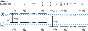
Figure 1: The system under consideration consists of $N$ two-level atoms, where the two states of half of the atoms have magnetic quantum numbers $m$ and $\tilde{m}$ and the other half have magnetic quantum numbers $-m$ and $-\tilde{m}$. A magnetic field leads to linear Zeeman shifts which are equal in magnitude but opposite in sign. The goal is to precisely estimate the transition frequency $\omega$.

$$|\psi_{in}\rangle=\left(\frac{1}{\sqrt{2}}\left(|0\rangle+|1\rangle\right)\right)^{\otimes N}$$ (3)

by applying a Hadamard gate to all atoms using two light fields (lasers or microwaves) of frequency $\omega_{L,a}$ and $\omega_{L,b}$ which might be slightly detuned from the atomic transition frequencies $\omega_{a}$ and $\omega_{b}$. In practice, the Hadamard gate would be realized by performing a $\pi/2$-pulse which is, strictly speaking, not the same as a Hadamard gate but the difference has no effect on the estimation uncertainty of $\omega$. After the Hadamard gate, the Hamiltonian of the system in a rotating frame takes the form

$$H=\frac{\delta_{a}}{2}\sum_{j\leq N/2}\sigma_{z}^{j}+\frac{\delta_{b}}{2}\sum_{j>N/2}\sigma_{z}^{j}$$ (4)

with $\delta_{i}\equiv\omega_{i}-\omega_{L,i}$, $i=a,b$. The system then evolves according to Eq. (1) for a ‘free evolution’ time $t$ before a second Hadamard gate and a measurement of the atoms in the $\{|0\rangle,\,|1\rangle\}$-basis is performed. In this paper it is assumed that $t$ is sufficiently large to let the system evolve into a stationary state. The whole procedure is repeated $\nu$ times leading to $\nu$ measurement results which provide, by using an appropriate estimator, an estimate $\omega_{est}$ of the transition frequency $\omega$. The statistical uncertainty $\Delta\omega$ of $\omega_{est}$ can be quantified by Braunstein94 ; Braunstein96

$$\Delta\omega=\left\langle\left(\frac{\omega_{est}}{|\partial\langle\omega_{est}\rangle/\partial\omega|}-\omega\right)^{2}\right\rangle^{1/2}$$ (5)

which, in the case of an unbiased estimator, is simply the standard deviation. The uncertainty, or precision, $\Delta\omega$ is bounded from below by the Cramér-Rao bound and the quantum Cramér-Rao bound Helstrom ; Braunstein94 ; Braunstein96

$$\Delta\omega \geq \frac{1}{\sqrt{\nu F}}=\frac{1}{\sqrt{TF/t}}\equiv\Delta\omega_{CR}$$ (6)

$$\geq \frac{1}{\sqrt{\nu F_{Q}}}=\frac{1}{\sqrt{TF_{Q}/t}}\equiv\Delta\omega_{QCR},$$ (7)

where $F$ is the Fisher information and $F_{Q}$ is the quantum Fisher information (QFI). Furthermore, $T\equiv\nu t$ is the total time of the experiment, where $t$ is the time needed for a single experimental run which for simplicity is assumed to be approximately equal to the free evolution time between the two Hadamard gates. The Fisher information $F$ depends on the state of the system before the measurement and the particular measurement we perform while the QFI depends only on the state before the measurement. The first bound in Eq. (7) can be reached via maximum likelihood estimation for large $\nu$ and the second bound by an optimal measurement which always exists Braunstein94 .

A word of caution is in order if the above model [i.e. Eq. (1)] is applied to the experimental setup described in Monz10 since there it has been pointed out that the magnetic field fluctuations leading to dephasing are non-Markovian. Nonetheless, it should be possible to apply the method described in this paper to the case Monz10 since it only relies on the stationary state (i.e. $\gamma t\gg 1$). This state will consist of an incoherent mixture of eigenstates of $L$ which will be the same for the Markovian and the non-Markovian case of Monz10 . Furthermore, we can always artificially enforce the noise to be of the form (1) such that the initial state relaxes quickly into the stationary state. Any additional non-Markovian fluctuations of the magnetic field should then have no effect.

III Benchmarks

In conventional Ramsey interferometry, i.e. if the same internal states for all atoms are used, and in the absence of magnetic field fluctuations, the best possible precision in case of a product state (3) turns out to be $1/\sqrt{TtN}$, i.e. the standard quantum limit. Using an $N$-particle GHZ state $|\psi_{in}^{GHZ}\rangle=(|0\rangle^{\otimes N}+|1\rangle^{\otimes N})/\sqrt{2}$ instead would ideally improve this precision to $1/\sqrt{Tt}N$, i.e. the Heisenberg limit Bollinger96 . However, if magnetic field fluctuations are taken into account this improvement is diminished significantly. In fact, if uncorrelated, Markovian dephasing with dephasing rate $\gamma$ is assumed it has been shown that the best possible precision in Ramsey interferometry is given by

$$\Delta\omega_{bench}=\sqrt{\frac{2\gamma\mathrm{e}}{NT}}$$ (8)

for both the product state (3) and the GHZ state, i.e. the two states are metrologically equivalent Huelga97 . It should be noted that Eq. (8) is based on the quantum Cramér-Rao bound which in this case is equal to the Cramér-Rao bound. Furthermore, in order to obtain expression (8), an optimal free evolution time $t=t_{opt}=1/2\gamma$ in case of a product state and $t=t_{opt}=1/2N\gamma$ in case of a GHZ state has been assumed.

In the presence of correlated dephasing as in Eq. (1) the situation gets even worse. In fact, it has been calculated numerically in Dorner12 that for a product state (3) the precision, i.e. the quantum Cramér-Rao bound, is given by

$$\Delta\tilde{\omega}_{bench}\approx(1.41+0.87/N^{0.90})\sqrt{\gamma/T},$$ (9)

and for a GHZ state a precision of $\sqrt{2\mathrm{e}\gamma/T}$ is obtained, none of which tend to zero for large $N$ Dorner12 . A solution to this problem was developed in Dorner12 , where it was shown that using a level scheme as in Fig. 1 and a GHZ state as input of the Ramsey interferometer the precision is given by $1/\sqrt{Tt}N\xi$, where $\xi$ is the preparation fidelity of the GHZ state. Although incredible progress has been made to create large GHZ states in ion traps Monz10 it is still a very challenging and expensive task to prepare such states. In the next sections I therefore present a method which requires merely the product state (3) which is easy to prepare in experiments. I will use Eq. (8) as a benchmark to measure the performance of the method since the corresponding scenario employs product states as well. Equation (9) will serve as a benchmark to a lesser extend since this precision is considerably worse than (8). A situation where (9) occurs as precision would therefore be avoided in practice. The precision of the method discussed in the next sections is not as good as $1/\sqrt{Tt}N\xi$, which relies on entanglement, but clearly beats the benchmarks (8) and (9).

IV Estimation precision

The method described in this paper relies on the stationary state resulting from the dynamics described by Eq. (1) given that the input state has the form (3). In the following I will first derive an expression for this state and then calculate the corresponding estimation uncertainties $\Delta\omega_{CR}$ and $\Delta\omega_{QCR}$. To ease notation, I will call the first $M=N/2$ atoms subsystem $A$ and the second $M$ atoms subsystem $B$. Additionally, it is helpful to realize that Eq. (1) and the state (3) are completely symmetric under particle exchange on subsystem $A$ and $B$, respectively. Therefore, a Fock representation can be introduced,

$$|k,M-k\rangle_{A}|l,M-l\rangle_{B}=$$

$$\frac{1}{\sqrt{c^{M}_{k}c^{M}_{l}}}\sum_{P}P|i_{1},i_{2},\ldots,i_{M}\rangle\sum_{P}P|i_{M+1},i_{M+2},\ldots,i_{N}\rangle,$$ (10)

where $c^{M}_{k}\equiv\binom{M}{k}$ and $i_{j}=0,1$ and $k$ ($N-k$) is the number of zeros (ones) in $|i_{1},i_{2},\ldots,i_{M}\rangle$ and analogously for $|i_{M+1},i_{M+2},\ldots,i_{N}\rangle$. Furthermore, both sums are over all permutations $P$ of particles which lead to different terms in each sum. Hence, the state $|k,M-k\rangle_{A}|l,M-l\rangle_{B}$ is a state with $k$ atoms in state $|0\rangle$ and $M-k$ atoms in state $|1\rangle$ on subsystem $A$ and $l$ atoms in state $|0\rangle$ and $M-l$ atoms in state $|1\rangle$ on subsystem $B$. To make the notation simpler, in the following I will use the abbreviations $|k\rangle_{A}\equiv|k,M-k\rangle_{A}$ and $|l\rangle_{B}\equiv|l,M-l\rangle_{B}$. In this representation the product state (3) is given by

$$|\psi_{in}\rangle=\frac{1}{2^{M}}\sum_{k,l=0}^{M}\sqrt{c^{M}_{k}c^{M}_{l}}|k\rangle_{A}|l\rangle_{B}.$$ (11)

In addition, the operators $\sum_{j\leq N/2}\sigma_{z}^{j}=a_{0}^{\dagger}a_{0}-a_{1}^{\dagger}a_{1}$ and $\sum_{j>N/2}\sigma_{z}^{j}=b_{0}^{\dagger}b_{0}-b_{1}^{\dagger}b_{1}$ can be introduced, where $a_{i}^{\dagger}$ ($a_{i}$) are bosonic creation (annihilation) operators of an atom in state $|i\rangle,\,i=0,1$ in subsystem $A$, and $b_{i}^{\dagger}$, $b_{i}$ act in the same way on subsystem $B$. Using the fact that $a_{0}^{\dagger}a_{0}+a_{1}^{\dagger}a_{1}=b_{0}^{\dagger}b_{0}+b_{1}^{\dagger}b_{1}=M$ the equation of motion is of the form (1) but now with

$$L=2(b_{0}^{\dagger}b_{0}-a_{0}^{\dagger}a_{0})$$ (12)

and

$$H=\delta(a_{0}^{\dagger}a_{0}+b_{0}^{\dagger}b_{0})+\tilde{\delta}(b_{0}^{\dagger}b_{0}-a_{0}^{\dagger}a_{0}),$$ (13)

where

$$\tilde{\delta} \equiv \frac{\omega_{b}-\omega_{a}}{2}-\frac{\omega_{L,b}-\omega_{L,a}}{2},$$ (14)

$$\delta \equiv \omega-\frac{\omega_{L,a}+\omega_{L,b}}{2}.$$ (15)

The state of the system at time $t$ is then given by

$$\rho(t)= \mathrm{e}^{-\mathrm{i}Ht}\mathrm{e}^{-\frac{\gamma}{4}L^{2}t}$$

$$\times\sum_{m=0}^{\infty}\frac{(\gamma t/2)^{m}}{m!}L^{m}|\psi_{in}\rangle\langle\psi_{in}|L^{m}\mathrm{e}^{-\frac{\gamma}{4}L^{2}t}\mathrm{e}^{\mathrm{i}Ht}$$

$$= \frac{1}{2^{N}}\sum_{k,l,j,n=0}^{M}\sqrt{c^{M}_{k}c^{M}_{l}c^{M}_{j}c^{M}_{n}}|k\rangle_{A}|l\rangle_{B}\langle j|_{A}\langle n|_{B}$$

$$\times\mathrm{e}^{-\gamma t(l-k+j-n)^{2}}\mathrm{e}^{-\mathrm{i}\tilde{\delta}t(l-k+j-n)}\mathrm{e}^{-\mathrm{i}\delta t(k+l-j-n)}$$ (16)

and the stationary state, i.e. $\gamma t\gg 1$, is therefore

$$\rho_{stat}= \frac{1}{2^{N}}\sum_{k,l,j,n=0}^{M}\sqrt{c^{M}_{k}c^{M}_{l}c^{M}_{j}c^{M}_{n}}|k\rangle_{A}|l\rangle_{B}\langle j|_{A}\langle n|_{B}$$

$$\times\mathrm{e}^{-\mathrm{i}\delta t(k+l-j-n)}\delta_{l+j,k+n}.$$ (17)

Note that this state does not depend anymore on $\tilde{\delta}$.

In the atomic basis $\rho_{stat}$ takes the form

$$\rho_{stat}=\sum_{k=0}^{N}p_{k}\mathrm{e}^{-\mathrm{i}Ht}|\psi_{k}\rangle\langle\psi_{k}|\mathrm{e}^{\mathrm{i}Ht},$$ (18)

where the $|\psi_{k}\rangle$ are eigenstates of $L$ which are symmetric in $A$ and $B$, respectively and the $p_{k}$ are the dimensions of the corresponding eigenspaces divided by $2^{N}$. The correlated noise removes all coherences of the initial state except for those which are unaffected by the noise. For example for $N=2$ this leads to

$$|\psi_{0}\rangle=\frac{1}{\sqrt{2}}(|00\rangle+|11\rangle),\,|\psi_{1}\rangle=|01\rangle,\,|\psi_{2}\rangle=|10\rangle$$ (19)

with $p_{0}=1/2,\,p_{1}=p_{2}=1/4$, and for $N=4$ we have

$$|\psi_{0}\rangle=\frac{1}{\sqrt{6}}(|0000\rangle+|0101\rangle+|0110\rangle$$

$$\qquad\qquad+|1001\rangle+|1010\rangle+|1111\rangle)$$

$$|\psi_{1}\rangle=\frac{1}{2}\left(|0100\rangle+|1000\rangle+|1101\rangle+|1110\rangle\right)$$

$$|\psi_{2}\rangle=\frac{1}{2}\left(|1011\rangle+|0111\rangle+|0010\rangle+|0001\rangle\right)$$

$$|\psi_{3}\rangle=|1100\rangle,\,|\psi_{4}\rangle=|0011\rangle$$ (20)

and $p_{0}=3/8,\,p_{1}=p_{2}=1/4,\,p_{3}=p_{4}=1/16$. As can be seen, for $N=2$ the stationary state $\rho_{stat}$ is a Bell state with 50% fidelity. This state (except for a bit flip of the second atom), also created by correlated dephasing, has been prepared in an experiment where it has been demonstrated that it can lead to improvements in the measurement of electric quadrupole moments and the line width of a laser Chwalla07 .

Based on $\rho_{stat}$ the QFI $F_{Q}$ can be calculated (see Appendix A) leading to

$$\Delta\omega_{QCR}=\frac{1}{\sqrt{TtN}}$$ (21)

which is the same expression as obtained for conventional Ramsey interferometry with a product state in the complete absence of dephasing. In other words, using the method discussed in this paper would ideally eliminate all negative influences of magnetic field fluctuations in the system. This result is based on the QFI and therefore does not necessarily correspond to the measurement scheme performed in Ramsey interferometry, i.e. Hadamard gate and detection of the state of the atoms. The performance of this particular measurement can be studied by calculating the Fisher information which is given by

$$F=\sum_{k,l=0}^{\frac{N}{2}}\frac{1}{p(k,l|\omega)}\left(\frac{d}{d\omega}p(k,l|\omega)\right)^{2},$$ (22)

where $p(k,l|\omega)$ is the probability to find $k$ excited atoms in $A$ and $l$ excited atoms in $B$ given that the value of the transition frequency is $\omega$,

$$p(k,l|\omega)=\langle k|_{A}\langle l|_{B}H_{g}^{\otimes N}\rho_{stat}(\omega)H_{g}^{\otimes N}|k\rangle_{A}|l\rangle_{B},$$ (23)

where $H_{g}$ is a Hadamard gate.

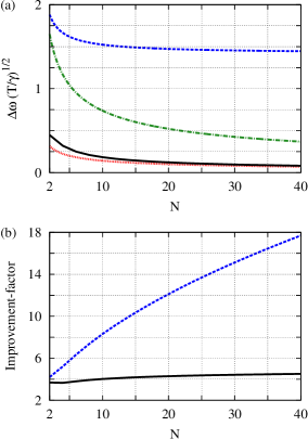
Figure 2: (a) Estimation uncertainty, $\Delta\omega$, depending on the number of atoms $N$ for $\gamma t=5$. The solid (black) line is the estimation uncertainty $\Delta\omega_{CR}$ based on the Fisher information (22). The dotted (red) line is the uncertainty $\Delta\omega_{QCR}$ based on the QFI and given by Eq. (21). The dash-dotted (green) line and the dashed (blue) line are the benchmarks (8) and (9), respectively. (b) Improvement factors $I$ (solid, black line) and $\tilde{I}$ (dashed, blue line) corresponding to the improvements over the benchmarks (8) and (9), respectively.

From Eqs. (17), (22) and (23) it is clear that the Fisher information has the form $F=t^{2}f(\delta t)$. The quantity $f(\delta t)$ can then be calculated numerically and maximized over $\delta t$, i.e.

$$f_{max}\equiv\underset{\delta t}{\max}f(\delta t),$$ (24)

which yields $\Delta\omega_{CR}$. A result is given by the solid (black) line in Fig. 2(a). As can be seen, the uncertainty $\Delta\omega_{CR}$ is slightly higher than the uncertainty based on the QFI, Eq. (21). This means that the measurement performed in Ramsey interferometry is not optimal. However, the measurement necessary to reach the precision (21) will be a non-trivial and, in general, non-local measurement which will be difficult to implement (and therefore, in practice, will have finite fidelity). In fact the maximum Fisher information follows approximately the behavior $f_{max}=a_{0}N+a_{1}$ where $a_{0}\approx 0.80\pm 0.005,\,a_{1}\approx-2.24\pm 0.12$ which is obtained by a fit to data between $N=8$ and $N=40$ obtained by numerically calculating $f_{max}$. For large $N$ this approximately yields

$$\Delta\omega_{CR}\approx\frac{1}{\sqrt{a_{0}TtN}}$$ (25)

which is only slightly higher (approximately by a factor 1.1) than Eq. (21). It is therefore questionable if a more complex measurement is worth the effort.

It should be emphasized again that the results (22) and (25) are equal or similar to those obtained for a completely noiseless system. Such an effect can, of course, also be achieved by using states which are inherently insensitive to magnetic fields, particularly ‘clock transitions’ which use states with zero magnetic quantum number. Therefore, the method presented in this paper removes the restriction to clock transitions and makes it possible to consider a greater variety of transitions for frequency standard experiments.

A comparison of the precision $\Delta\omega_{CR}$ based on the Fisher information (22) and the benchmarks (8) and (9) is shown in Fig. 2(b). More precisely, the solid (black) line shows the improvement factor $I\equiv\Delta\omega_{bench}/\Delta\omega_{CR}$ and the dashed (blue) line shows $\tilde{I}\equiv\Delta\tilde{\omega}_{bench}/\Delta\omega_{CR}$ for $\gamma t=5$ which means that the atoms can be kept 5 times longer than the coherence time of a single atom. Unsurprisingly, $\tilde{I}$ grows with $N$ since $\Delta\tilde{\omega}_{bench}$ approaches a constant, non-zero value for large $N$. The improvement factor $I$ on the other hand, converges to a constant value since both precisions scale like $\sqrt{N}$ for large $N$. In particular, for $N\gg 1$ the improvement factors are

$$I \approx \sqrt{2\mathrm{e}\gamma t}\sqrt{a_{0}+\frac{a_{1}}{N}}\approx 2.09\sqrt{\gamma t},$$ (26)

$$\tilde{I} \approx \left(1.41+\frac{0.87}{N^{0.90}}\right)\sqrt{\gamma t(Na_{0}+a_{1})}\approx 1.26\sqrt{N\gamma t}.\qquad$$ (27)

Both improvement factors are proportional to $\sqrt{\gamma t}$ which can be considerably larger than in conventional Ramsey interferometry since there is no restriction due to the decoherence caused by magnetic field fluctuations. In fact, it is the noise which generates the state which is used and the improvement factor can therefore be significant.

V Imperfect gates and measurements

In the previous sections imperfections of the Hadamard gates and imperfect measurements of the internal states of the atoms have been neglected. An imperfect Hadamard gate can be modeled by

$$\mathcal{E}_{H}(\rho)=\eta_{H}H_{g}\rho H_{g}+\frac{1}{2}(1-\eta_{H})\openone,$$ (28)

where $H_{g}$ is a perfect Hadamard gate and $\eta_{H}$ characterizes the probability to have a perfect gate. A faulty measurement of an atom can be modeled using the measurement operators

$$\Pi_{i}=\frac{1}{2}(1+\eta_{M})|i\rangle\langle i|+\frac{1}{2}(1-\eta_{M})\sigma_{x}|i\rangle\langle i|\sigma_{x},$$ (29)

where $i=0,1$, and $\eta_{M}$ is the likeliness that the correct

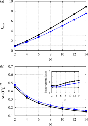
Figure 3: (a) Maximum Fisher information $f_{max}$ defined by Eq. (24) for $\eta_{M}=\eta_{H}=1$ (solid, black line) and $\eta_{M}=\eta_{H}=0.99$ (dashed, blue line) depending on the number of atoms $N$. (b) Estimation uncertainty $\Delta\omega_{CR}$ for $\eta_{M}=\eta_{H}=1,\,\gamma t=5$ (solid, black line) and estimation uncertainty $\Delta\omega_{CR}$ for $\eta_{M}=\eta_{H}=0.99,\,\gamma t=5$. Inset: Improvement factors $I$ (solid, black line) and $I_{\eta_{M},\eta_{H}}$ (dashed, blue line).

measurement result is obtained. Both measurement and Hadamard gate can now be performed routinely with very high fidelities. Indeed, with current ion trap technology gate and readout fidelities in excess of $\eta_{H}=\eta_{M}\approx 0.99$ have been achieved Lucas10 . Note that errors in the state initialization preceding the first Hadamard gate can be absorbed into these quantities. However, this initialization, which is typically done via optical pumping, can be done with very high fidelities even exceeding those of gate and measurement. Furthermore, it should be emphasized that throughout this paper it is assumed that exactly half of the atoms are in group $A$ and half of the atoms are in group $B$. This requires that group $A$ and $B$ can be addressed separately during the initialization phase which can be easily achieved with current ion trap technology. Despite the fact that $\eta_{H}$ and $\eta_{M}$ are close to one it has been shown previously that they can have a significant effect on the overall estimation precision. For example, in the method discussed in Dorner12 which relies on highly entangled GHZ states, these imperfections increase the estimation uncertainty by a factor $(\eta_{M}\eta_{H})^{N}$, i.e. exponentially with the number of atoms. Fortunately, if separable states are used, it is to be expected that these imperfections have a much smaller effect. For example, the benchmark (8), which is based on a product state, is now given by $\Delta\omega_{bench}^{\eta_{M},\eta_{H}}=\sqrt{2\gamma\mathrm{e}/NT}/\eta_{M}\eta_{H}^{2}$ Dorner12 . Hence it is merely reduced by a factor $\eta_{M}\eta_{H}^{2}$ which is independent of $N$ and therefore has only a minor effect if $\eta_{H}$ and $\eta_{M}$ are close to $1$.

In order to study the effect of imperfect measurements and Hadamard gates on the method discussed in this paper, numerical calculations of $f_{max}$ in the atomic basis have been performed for $\eta_{H,M}$ different from $1$. An example is shown in Fig. 3 (dashed, blue line) depending on $N$ and for $\eta_{H}=\eta_{M}=0.99$. The dashed line shows an approximately linear behaviour with respect to $N$ for $N\gtrsim 8$, i.e. $f_{max}\approx\tilde{a}_{0}N+\tilde{a}_{1}$, where $\tilde{a}_{0},\,\tilde{a}_{1}$ are approximately independent of $N$. As a reference, $f_{max}$ for $\eta_{H}=\eta_{M}=1$ is plotted as well (black line) which corresponds to the black line in Fig. 2(a) which also shows a linear behaviour as discussed in Sec. IV. This shows that the precision still scales like the standard quantum limit, $\Delta\omega_{CR}\sim 1/\sqrt{\tilde{a}_{0}N+\tilde{a}_{1}}$ and therefore $\eta_{M,H}$ have only a minor effect on the overall estimation precision if they are close to $1$. $\Delta\omega_{CR}$ is shown in Fig. 3(b) (dashed, blue line). The loss in precision for $\eta_{H}=\eta_{M}=0.99$ is small: It is merely a factor $1.09$ for $N=14$. The improvement factor $I_{\eta_{M},\eta_{H}}\equiv\Delta\omega_{bench}^{\eta_{M},\eta_{H}}/\Delta\omega_{CR}$ is shown in the inset of Fig. 3(b) (dashed, blue line) together with $I$ (black line) which is the same as the black line in Fig. 2. For example, for $N=14$ the improvement factor is reduced from $4.16$ to $3.94$.

VI The effect of spontaneous emission

It was shown in the previous sections that the improvement factors $I$ and $\tilde{I}$ increase with $\sqrt{\gamma t}$. The value of $\gamma t$ will be limited by a decay of the excited atomic state caused by spontaneous emission with a decay time $1/\Gamma$. References Chwalla07 and Monz10 report $1/\gamma$ to be a few milliseconds and $8$ms, respectively (the latter can be increased to $95\,$ms Monz10 ). The lifetime of the excited atomic state in these experiments is $1/\Gamma=1.17s$. For example, for $1/\gamma=5\,$ms the spontaneous decay time is therefore $\gamma/\Gamma\approx 230$ times larger than the dephasing time $1/\gamma$.

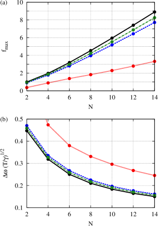
Figure 4: (a) Maximum Fisher information $f_{max}$ [see Eq. (24)] for $\Gamma=0$ (solid, black line), $\gamma/\Gamma=100$ (dashed, blue line), $\gamma/\Gamma=200$ (dashed-dotted, green line) and $\gamma/\Gamma=10$ (dotted, red line) depending on the number of atoms $N$ ($\eta_{M}=\eta_{H}=1$ and $\gamma t=5$ in all cases). (b) Estimation uncertainty $\Delta\omega_{CR}$ corresponding to the curves shown in (a).

Spontaneous emission can be included in our model by adding the term

$$\Gamma\sum_{j=1}^{N}\left(\sigma_{-}^{j}\rho\sigma_{+}^{j}-\frac{1}{2}\sigma_{+}^{j}\sigma_{-}^{j}\rho-\frac{1}{2}\rho\sigma_{+}^{j}\sigma_{-}^{j}\right)$$ (30)

to the equation of motion (1), where $\sigma_{\pm}=(\sigma_{x}\pm\mathrm{i}\sigma_{y})/2$. The fisher information $f_{max}$ can then be calculated numerically and results are shown in Fig. 4(a) for $\gamma t=5$ and $\gamma/\Gamma=200$ (dashed-dotted, green line), $\gamma/\Gamma=100$ (dashed, blue line) and $\gamma/\Gamma=10$ (dotted, red line) ($\eta_{M}=\eta_{H}=1$). The behavior is similar to that shown in Fig. 3(a), i.e. $f_{max}$ is approximately linear and the loss in precision is approximately independent of $N$ for $N\gtrsim 8$. The corresponding estimation uncertainties $\Delta\omega_{CR}$ are shown in Fig. 4(b). For example for $N=14$ the uncertainty is increased by a factor $1.04$ for $\gamma/\Gamma=200$, $1.07$ for $\gamma/\Gamma=100$ and $1.64$ for $\gamma/\Gamma=10$.

Unsurprisingly, numerical simulations reveal that the Fisher information $f_{max}$ decreases with increasing $\Gamma t$ but only for $N=2$ does it exhibit an exponential decay ($f_{max}\sim\exp(-2\Gamma t)$). For $N>2$ the decay is neither exponential nor does it follow a power law. Taking into account spontaneous emission and imperfect gates and measurements the benchmark (8) has to be modified to $\Delta\omega_{bench}^{\eta_{M},\eta_{H},\Gamma}=\sqrt{(2\gamma+\Gamma)\mathrm{e}/NT}/\eta_{M}\eta_{H}^{2}$. The improvement factor $I_{\eta_{M},\eta_{H},\Gamma}\equiv\Delta\omega_{bench}^{\eta_{M},\eta_{H},\Gamma}/\Delta\omega_{CR}$ is then given by

$$I_{\eta_{M},\eta_{H},\Gamma}=\sqrt{\frac{\gamma}{\Gamma}+\frac{1}{2}}\sqrt{\frac{2\mathrm{e}}{N}}\frac{1}{\eta_{M}\eta_{H}^{2}}\sqrt{\Gamma tf_{max}}.$$ (31)

Since $f_{max}$ is decreasing with $\Gamma t$ the term $\Gamma tf_{max}$ has a maximum which corresponds to an optimal free evolution time $t_{opt}$. Improvement factors for $N=2,\ldots,14$ (bottom to top) are shown in Fig. 5.

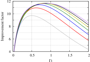
Figure 5: Improvement factor $I_{\eta_{M},\eta_{H},\Gamma}$ given by Eq. (31) versus $\Gamma t$ for $N=2,\ldots,14$ (bottom to top) and $\eta_{H}=\eta_{M}=0.99,\,\gamma/\Gamma=200$.

These examples take into account imperfect gates and measurements with $\eta_{H}=\eta_{M}=0.99$. For $\gamma/\Gamma=200$, the maxima of the curves yield optimal improvement factors $I_{\eta_{M},\eta_{H},\Gamma}=9.7,\,10.93,\,11.42,\,11.62,\,11.68,\,11.67,\,11.63$ for $N=2,\ldots,14$ corresponding to $\gamma t_{opt}=100,\,123,\,140,\,155,\,167,\,177,\,186$. Note that the location of the maxima, i.e. $\Gamma t_{opt}$, is independent of $\gamma/\Gamma$. For $\gamma/\Gamma=10$ we get the optimal improvement factors $I_{\eta_{M},\eta_{H},\Gamma}=2.22,\,2.5,\,2.61,\,2.66,\,2.67,\,2.67,\,2.66$ for $N=2,\ldots,14$ corresponding to $\gamma t_{opt}=5,\,6.2,\,7,\,7.8,\,8.4,\,8.9,\,9.3$. As can be seen, for example for $\gamma/\Gamma=200$, the optimal improvement factor peaks at a value of $11.68$ for $N=10$ and then decreases slightly. If this tendency persists the best possible advantage over conventional Ramsey interferometry is achieved for $N=10$. However, the behavior of $I_{\eta_{M},\eta_{H},\Gamma}$ for $N>14$ is not known. In the worst case the optimal improvement factor drops further. However, for the method described in this paper to be worse than conventional Ramsey interferometry, the optimal improvement factor would have to drop to a value of below one. The precision is given by $\Delta\omega_{CR}=c/\sqrt{N}I_{\eta_{M},\eta_{H},\Gamma}$ (with $c=\sqrt{(2\gamma+\Gamma)\mathrm{e}/T}/\eta_{M}\eta_{H}^{2}$). Thus, if the optimal $I_{\eta_{M},\eta_{H},\Gamma}$ does not change substantially for $N>14$, the corresponding optimal precision decreases approximately with $\sqrt{N}$.

VII Conclusions

I have shown that, by using a stationary state which is created by correlated dephasing which represents a significant source of noise in recent experiments with strings of trapped ions Monz10 ; Chwalla07 ; Roos06 ; Leibfried04 ; Langer05 ; Kielpinski01 , an improvement in the precision compared to standard Ramsey interferometry can be gained. This is due to the fact that the measurement precision essentially behaves as in a completely noiseless system, i.e. the precision is approximately given by $1/\sqrt{TtN}$. On the other hand, in standard Ramsey interferometry (under the influence of uncorrelated, Markovian dephasing) the free evolution time is limited by the coherence time of the system, $t\sim 1/\gamma$, leading to a precision proportional to $\sqrt{\gamma/NT}$. By comparing the two situations it is obvious that an improvement proportional to $\sqrt{\gamma t}$ can be gained. This gain is achieved at very low cost: The initial state is merely a product state of $N$ atoms, created by optically pumping two groups of atoms into two different internal states with magnetic quantum number $m$ and $-m$, and a subsequent Hadamard gate.

However, apart from correlated dephasing, further imperfections have to be expected in practice. In particular, I took into account imperfect Hadamard gates, imperfect measurements of the atomic states and spontaneous emission. The effect of imperfect gates and measurements is very small. It diminishes the estimation precision merely by a constant factor independent of $N$ (approximately $1.1$ for $\eta_{H,M}=0.99$). The effect on the improvement factor, i.e. the ratio of the precision of conventional Ramsey interferometry and the precision of the method discussed in this paper, is small as well. For example, for $\gamma t=5$ and $N=14$ atoms, the improvement factor is reduced from 4.16 to 3.94. The effect of spontaneous emission is to limit the free evolution time $t$ in the Ramsey interferometer. The examples shown in Figs. 2 and 3 assume $\gamma t=5$ which is a very conservative assumption. Recent experiments use transitions with a spontaneous decay time exceeding $1\,$s Chwalla07 which is about 200 times larger than the dephasing time. Under such circumstances I showed that, e.g. for $N=10$ atoms, the free evolution time can be extend to $\gamma t=167$. In conventional Ramsey interferometry the corresponding optimal evolution time would be merely $\gamma t=0.5$. This leads to an improvement in the estimation precision of one order of magnitude compared to standard Ramsey interferometry.

A further source of noise are phase or frequency fluctuations of the local oscillator. Since the local oscillator is the same for all atoms, its fluctuations will effectively lead to correlated dephasing, since all atoms are affected in the same way. This can be seen as fluctuating frequency shifts of all atoms which are equal in magnitude and have the same sign. This dephasing is of course independent of magnetic quantum numbers and, for example, would also be present if these are zero, i.e. if ‘clock-transitions’ are used. However, laser linewidths of about $\lesssim 1\,$Hz are now experimentally available which renders the effect of this form of noise very limited. Furthermore, a variation of the method presented in this paper which is adapted from Chwalla07 ; Roos06 could be used: If all atoms fluctuate in the same way the stationary state would have the same form as the one discussed in this paper except that half of the atoms would be ‘spin-flipped’. As a consequence, however, the quantity which can be estimated is not the arithmetic mean of two frequencies but the difference between two frequencies.

The stationary state used in this paper is not entangled, however, it has recently been pointed out that correlated noise can create quantum discord Lanyon13 . Whether the state considered in this paper contains such non-classical correlations and whether they are the reason for its superior performance in frequency estimation, is a subject for future research.

Appendix A Quantum Fisher information

Consider a system state $\rho$ which depends on a parameter $\omega$ which is to be estimated. The QFI is then given by Helstrom ; Holevo ; Braunstein94 ; Braunstein96

$$F_{Q}=\sum_{j,k;\,p_{k}+p_{j}\neq 0}\frac{2}{p_{j}+p_{k}}\left|\left\langle\phi_{j}\left|\frac{d}{d\omega}\rho\right|\phi_{k}\right\rangle\right|^{2}.$$ (32)

where $p_{k}$ and $|\phi_{k}\rangle$ are the eigenvalues and eigenvectors of $\rho$, respectively. The state $\rho_{stat}$ given by Eq. (17) can be diagonalized,

$$\rho_{stat}=\sum_{p=0}^{M}f_{p}|\phi_{p}^{0}\rangle\langle\phi_{p}^{0}|+\sum_{p=0}^{M-1}f_{p}|\tilde{\phi}_{p}^{0}\rangle\langle\tilde{\phi}_{p}^{0}|$$ (33)

with

$$f_{p} = \frac{1}{2^{N}}c^{N}_{p},$$ (34)

$$|\phi_{p}^{0}\rangle = \frac{1}{\sqrt{c^{N}_{p}}}\sum_{j=0}^{p}\sqrt{c^{M}_{j}c^{M}_{p-j}}\mathrm{e}^{-2\mathrm{i}j\delta t}|j\rangle_{A}|M-p+j\rangle_{B},$$ (35)

$$|\tilde{\phi}_{p}^{0}\rangle = \frac{1}{\sqrt{c^{N}_{p}}}\sum_{j=0}^{p}\sqrt{c^{M}_{j}c^{M}_{p-j}}\mathrm{e}^{2\mathrm{i}j\delta t}|M-j\rangle_{A}|p-j\rangle_{B}.\qquad\quad$$ (36)

The states $|\phi_{p}^{0}\rangle,\,|\tilde{\phi}_{p}^{0}\rangle$ are orthogonal to each other but to obtain a complete orthonormal basis set the states $|\phi_{p}^{k}\rangle,\,|\tilde{\phi}_{p}^{k}\rangle,\,k=1,\ldots,p$ have to be included which are eigenstates of $\rho_{stat}$ with eigenvalue $0$, i.e.

$$\langle\phi_{p}^{k}|\phi_{p^{\prime}}^{k^{\prime}}\rangle = \delta_{pp^{\prime}}\delta_{kk^{\prime}}$$ (37)

$$\langle\phi_{p}^{k}|\tilde{\phi}_{p^{\prime}}^{k^{\prime}}\rangle = 0.$$ (38)

The quantum Fisher information then takes the form

$$F_{Q}= 4t^{2}\sum_{p=0}^{M}f_{p}\sum_{k=1}^{p}\langle\phi_{0}^{p}|a_{0}^{\dagger}a_{0}+b_{0}^{\dagger}b_{0}|\phi_{k}^{p}\rangle$$

$$+4t^{2}\sum_{p=0}^{M-1}f_{p}\sum_{k=1}^{p}\langle\tilde{\phi}_{0}^{p}|a_{0}^{\dagger}a_{0}+b_{0}^{\dagger}b_{0}|\tilde{\phi}_{k}^{p}\rangle.$$ (39)

The above expression can be evaluated leading to the simple result $F_{Q}=Nt^{2}$ and therefore

$$\Delta\omega_{QCR}=\frac{1}{\sqrt{\nu N}t}=\frac{1}{\sqrt{TtN}}.$$ (40)

References

- (1) V. Giovannetti, S. Lloyd, and L. Maccone, Science 306, 1330 (2004)
- (2) J. P. Dowling, Contemp. Phys. 49, 125 (2008)
- (3) J. J. Bollinger, W. M. Itano, D. J. Wineland, and D. J. Heinzen, Phys. Rev. A 54, R4649 (1996)
- (4) M. Chwalla, K. Kim, T. Monz, P. Schindler, M. Riebe, C. Roos, and R. Blatt, Appl. Phys. B 89, 483 (2007)
- (5) D. Leibfried, M. D. Barrett, T. Schaetz, J. Britton, J. Chiaverini, W. M. Itano, J. D. Jost, C. Langer, and D. J. Wineland, Science 304, 1476 (2004)
- (6) C. F. Roos, M. Chwalla, K. Kim, and R. Blatt, Nature 443, 316 (2006)
- (7) V. Meyer, M. A. Rowe, D. Kielpinski, C. A. Sackett, W. M. Itano, C. Monroe, and D. J. Wineland, Phys. Rev. Lett. 86, 5870 (2001)
- (8) I. D. Leroux, M. H. Schleier-Smith, and V. Vuletić, Phys. Rev. Lett. 104, 250801 (2010)
- (9) A. Louchet-Chauvet, J. Appel, J. J. Renema, D. Oblak, N. Kjaergaard, and E. S. Polzik, New J. Phys. 12, 065032 (2010)
- (10) C. Gross, T. Zibold, E. Nicklas, J. Estéve, and M. K. Oberthaler, Nature 464, 1165 (2010)
- (11) M. F. Riedel, P. Böhi, Y. Li, T. W. Hänsch, A. Sinatra, and P. Treutlein, Nature 464, 1170 (2010)
- (12) Note that in case of non-linear systems the Heisenberg limit can be surpassed, S. Boixo, S. T. Flammia, C. M. Caves, and J. Geremia, Phys. Rev. Lett. 98, 090401 (2007)
- (13) U. Dorner, R. Demkowicz-Dobrzanski, B. J. Smith, J. S. Lundeen, W. Wasilewski, K. Banaszek, and I. A. Walmsley, Phys. Rev. Lett. 102, 040403 (2009)
- (14) N. Thomas-Peter, B. J. Smith, A. Datta, L. Zhang, U. Dorner, and I. A. Walmsley, Phys. Rev. Lett. 107, 113603 (2011)
- (15) T. Monz, P. Schindler, J. T. Barreiro, M. Chwalla, D. Nigg, W. A. Coish, M. Harlander, W. Hänsel, M. Hennrich, and R. Blatt, Phys. Rev. Lett. 106, 130506 (2011)
- (16) C. Langer, R. Ozeri, J. D. Jost, J. Chiaverini, B. DeMarco, A. Ben-Kish, R. B. Blakestad, J. Britton, D. B. Hume, W. M. Itano, D. Leibfried, R. Reichle, T. Rosenband, T. Schaetz, P. O. Schmidt, and D. J. Wineland, Phys. Rev. Lett. 95, 060502 (2005)
- (17) D. Kielpinski, V. Meyer, M. A. Rowe, C. A. Sackett, W. M. Itano, C. Monroe, and D. J. Wineland, Science 291, 1013 (2001)
- (18) S. F. Huelga, C. Macchiavello, T. Pellizzari, A. K. Ekert, M. B. Plenio, and J. I. Cirac, Phys. Rev. Lett. 79, 3865 (1997)
- (19) Y. Matsuzaki, S. C. Benjamin, and J. Fitzsimons, Phys. Rev. A 84, 012103 (2011)
- (20) A. W. Chin, S. F. Huelga, and M. B. Plenio, Phys. Rev. Lett. 109, 233601 (2012)
- (21) C. F. Roos(2005), arXiv:quant-ph/0508148
- (22) U. Dorner, New J. Phys. 14, 043011 (2012)
- (23) D. Leibfried, E. Knill, S. Seidelin, J. Britton, R. B. Blakestad, J. Chiaverini, D. B. Hume, W. M. Itano, J. D. Jost, C. Langer, R. Ozeri, R. Reichle, and D. J. Wineland, Nature 438, 639 (2005)
- (24) S. L. Braunstein and C. M. Caves, Phys. Rev. Lett. 72, 3439 (1994)
- (25) S. L. Braunstein, C. M. Caves, and G. J. Milburn, Ann. Phys. (NY) 247, 135 (1996)
- (26) C. W. Helstrom, Quantum Detection and Estimation Theory (Academic, New York, 1976)
- (27) A. H. Burrell, D. J. Szwer, S. C. Webster, and D. M. Lucas, Phys. Rev. A 81, 040302 (2010)
- (28) B. P. Lanyon, P. Jurcevic, C. Hempel, M. Gessner, V. Vedral, R. Blatt, and C. F. Roos(2013), arXiv:1304.3632 [quant-ph]
- (29) A. S. Holevo, Probabilistic and Statistical Aspects of Quantum Theory (North-Holland, Amsterdam, 1982)