A Transferable H₂O Interaction Potential Based on a Single Center Multipole Expansion: SCME

Abstract

A transferable potential energy function for describing the interaction between water molecules is presented. The electrostatic interaction is described rigorously using a multipole expansion. Only one expansion center is used per molecule to avoid the introduction of monopoles. This single center approach turns out to converge and give close agreement with ab initio calculations when carried out up to and including the hexadecapole. Both dipole and quadrupole polarizability is included. All parameters in the electrostatic interaction as well as the dispersion interaction are taken from ab initio calculations or experimental measurements of a single water molecule. The repulsive part of the interaction is parametrized to fit ab initio calculations of small water clusters and experimental measurements of ice I_h. The parametrized potential function was then used to simulate liquid water and the results agree well with experiment, even better than simulations using some of the point charge potentials fitted to liquid water. The evaluation of the new interaction potential for condensed phases is fast because point charges are not present and the interaction can, to a good approximation, be truncated at a finite range.

1 Introduction

Water in its various forms plays a fundamental role in many biological, chemical and physical processes[1]. Hydration water around biomolecules participates actively in biological function such as protein folding [2], and the complex interactions between biomolecules inside cells is mediated by the water solvent through the hydrophobic effect[3, 4, 5]. Supercooled water in the bulk and in confined geometries is also of large current interest due to the intriguing yet controversial possibility of a liquid-liquid critical point in the deeply supercooled region[6, 7, 8]. On a larger scale, global climate change is affected by feedback loops involving water vapor — the most common greenhouse gas — and liquid water [9, 10]. Moreover, our environment depends critically on the properties of ice [11, 12], both through the rheology of ice sheets[13] and the meteorology of clouds[14]. Ice is also found in interstellar space, where, in an amorphous phase, it coats dust grains in molecular clouds[15, 16]. These coatings can serve as a substrate for the formation of chemicals of biological interest[17]. In spite of the large amounts of information available, the molecular mechanisms behind all of these processes are just beginning to be understood.

The water molecules involved in the most common processes in nature are in an environment that is characteristic of neither liquid water, ice nor water vapor, e.g. amorphous ice[18, 19, 20, 21, 22, 8], premelted[23, 24, 25] and solid[26, 27, 28] surfaces and adsorbed overlayers. The correct description of such systems is in many cases beyond the computational capabilities of available ab initio methods. Nowadays most condensed phase systems are studied by means of density functional theory (DFT)[29, 30] or model potentials[31]. In the case of water, however, DFT methods are handicapped by both theoretical and practical reasons[32]: first, the results obtained for systems containing hydrogen bonds are rather mixed [33, 34, 35, 36, 37, 38]. Secondly, the most commonly used functionals do not correctly account for the long-range $R^{-6}$ terms corresponding to the dispersion energy, and are therefore unable to correctly model weak intermolecular interactions[39, 40]. A new class of so called vdW functionals that include a description of non-local interactions have been introduced[41, 42, 43, 44], but their accuracy is still subject to debate and for many applications the computational demands are too high.

Interaction potential functions, on the other hand, usually have low computational requirements and have been successful in modeling various aspects of water[45, 46]. The functions most commonly used are simple two-body effective potentials such as SPC/E[47], TIP3P[48] and TIP4P[48] (and more recently improved reparametrizations such as TIP4P/Ew[49] and TIP4P/2005[50]) which were developed to reproduce the structural and thermodynamic properties of bulk phases at ambient temperature and pressure. A common feature of these potentials is enhanced multipole moments of the molecules representing the effects of the mean-field, many-body polarization seen in the liquid and the solid. Although this approach gives reasonable results for several properties of the bulk phase, it has been shown that the explicit introduction of many-body polarization effects is required to accurately describe other environments, for example water clusters[51, 52, 53, 54]. Pedulla and Jordan[51] have shown that non-additive interactions play an important role in the description of phase changes in small clusters, an observation that is likely to extend to processes such as premelting, island formation on surfaces and diffusion. Polarizable model potentials such as NCC[55] and DC[54] have been shown to give good results for both small clusters and the liquid, and modifications of the DC potential provide an acceptable description of ice[56]. More recently Millot et al.[57, 58] and Burnham and Xantheas[59, 60, 61] have presented transferable potentials that reproduce well ab initio results for clusters.

An important concern when modeling condensed phases is long range interactions, i.e. the interaction between atoms and molecules separated by large distance. The contribution of such long range interactions, beyond a cutoff radius of $R_{c}$, to the energy of the system can be obtained by integration as

$$U^{\text{tail}}(R_{c})~{}\propto~{}\int_{R_{c}}^{\infty}u(R)~{}4\pi R^{2}~{}dR,$$ (1)

where $u(R)$ is the interaction potential function. If the potential decays faster than $R^{-3}$ a value for $R_{c}$ can be determined in such a way that the long range contribution becomes insignificant and only interactions for distances smaller than $R_{c}$ need to be included. The vast majority of empirical water potentials functions, however, make use point or diffuse charges on atomic or pseudo-atomic sites, resulting in an interaction between sites that decays as $R^{-1}$. The contribution of this long range tail then diverges and its effects must be accounted for explicitly. Several methods have been developed for this purpose, varying in their rigor and computational effort, and their relative merits have been the subject of much debate. The most widely used approaches, such as Ewald sums[62, 63] and reaction field methods, add a significant computational effort. Moreover, the use of periodic boundary conditions in the case of the Ewald method might introduce artificial periodicity effects such as dynamic correlations between images. The simplest procedure, i.e. truncation of the long-range interactions due to the point or diffuse charges, is known to result in spurious behavior at the cutoff distance[64].

The widespread use of point charges in model potentials has been a matter of convenience rather than necessity since the leading term in the electrostatic multipole expansion for a water molecule is the dipole and the long range interaction consequently decays as $R^{-3}$. Therefore, the integral in Equation 1 can converge in certain cases for a model potential that avoids point or diffuse charges. Two systems of special interest for which such a truncation scheme should be feasible are proton disordered crystals, and surfaces. In the former the long-range interactions tend to cancel out due to the random orientation of the molecular dipoles, while for surfaces the volume integral in Equation 1 becomes two-dimensional and converges unconditionally. The use of charge free potentials is not new. Dipolar fluids are commonly simulated using Stockmayer-type potentials composed of a Lennard-Jones interaction supplemented with an embedded point dipole moment. An example of this approach is the ”soft sticky dipole” model of Liu and Ichiye[65]. These potentials suffer from the drawback that they are parametrized to reproduce average properties of bulk water and, for the most part, are not polarizable and, therefore, not transferable. A different approach is the so-called polarizable electropole of Barnes et al.[66] involving a simple approximation to the multipole expansion based on polarizable dipoles and quadrupoles. This potential is, however, not of high accuracy and has not been used much.

Previous studies of a charge free, single-center multipole expansion for the water monomer[67, 68] have shown that an accurate description of the electric fields in ice and around water clusters is obtained if the expansion is carried out up to and including the hexadecapole. Due to the proton-disordered nature of ice Ih, the local electric field at a water molecule due to its surroundings was shown to be converged for a cutoff radius of only 8 Å[67]. This approach has several advantages over the distributed multipole expansion[57, 58], where two or more centers of a multipole expansion are placed on each molecule. For example, the use of a single center requires significantly less computational effort in the iterative solution of the polarization equations. Secondly, since no point charges are present and the long range interaction therefore decays quickly, it is possible to introduce a finite range cutoff, $R_{c}$, and avoid the computationally demanding Ewald summation.

In the present article, we extend these studies and present a complete model potential function where the electrostatic and induction parameters are obtained for a single water molecule, thus allowing the condensed phase properties to emerge from the molecular properties through polarizability and self-consistent calculations of the local field. This construction of the potential function ensures transferability to different kinds of environments, while the truncation of long range interactions makes it easier to carry out long simulations on complex systems. The goal is to create a potential energy function that reproduces accurate ab initio calculations of the Born-Oppenheimer potential surface. Quantum mechanical effects such as zero-point energy are not built into the potential, unlike for example the SPC/E and TIP4P potentials where the fitting to experimental data indirectly brings in some average quantum mechanical effects, appropriate only for bulk water at ambient conditions. In the following section we describe the different components of the potential in detail, as well as the various procedures used to obtain the parameters involved. Section 3 presents and discusses the results for the (H₂O)_n clusters with $n=2$ to $6$ (with special emphasis on the dimer), liquid water and ice Ih, the most common crystal structure of ice. Finally, Section 4 presents conclusions and future perspectives.

2 Definition of the Potential Function

The vast majority of interaction potentials are based in one way or another on the long- and short-range perturbation theories of intermolecular interactions [69]. The former applies when the separation between molecules is sufficiently large for the overlap between wave functions to be insignificant. In such a case the exact expression for the interaction energy reduces to a sum of electrostatic, induction and dispersion terms. At shorter distances, however, the exchange repulsion and in some cases the charge-transfer arising from the overlap cannot be ignored. Since the evaluation of the interaction at intermediate and short range is difficult, the electrostatic, induction and dispersion terms arising from the long-range perturbation theory are often simply scaled by means of damping functions at short range and complemented by a short-range repulsion[70]. With the exception of the ASP family of model interaction potentials[57, 58], the charge-transfer component is not explicitly included and is usually folded into the other components through the parametrization, a simplification which is justified due to the small magnitude of this effect[71].

Following this approach, we have defined the total interaction energy between water molecules as the sum of electrostatic, induction, dispersion and short-range repulsion terms:

$$E_{\text{tot}}~{}=~{}E_{\text{es+ind}}+E_{\text{disp}}+E_{\text{rep}}~{}.$$ (2)

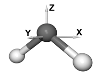
Figure 1: Molecular Cartesian coordinate system with origin in the center of mass used in the definition of the multipole moments and polarizabilities.

Each water molecule is treated as a rigid body with fixed bond length and bond angle. We have chosen the experimentally determined molecular conformation ($r_{\text{OH}}=0.9572\text{\AA}$, $\widehat{\text{HOH}}=104.52$^∘) to define the center of mass, but the interaction potential presented here is independent of that choice. A Cartesian coordinate system with origin on the center of mass is defined as shown in Figure 1. The center of mass was used as a reference point in the calculation of the of electrostatic and induction components. The other components, i.e. the dispersion and repulsion, are naturally centered on the oxygen atom. Two auxiliary centers are used simply to orient the multipole moments associated with each monomer and are located on the hydrogen atoms.

2.1 Electrostatic and Induction Energies

The electric interaction between the molecules is described in terms of a single-center multipole expansion. The molecules are modeled as a collection of multipole moments located at the centers of mass. Previous calculations[67, 68] have demonstrated that in order to reach convergence in the multipole expansion of the electric field at the relevant intermolecular distances, the expansion had to be carried out up to and including the hexadecapole moment. Dipole-dipole, dipole-quadrupole and quadrupole-quadrupole polarizabilities were included to account for the induction effects. Within this approximation, the electrostatic+induction component takes the following form:

$$E_{\text{es+ind}}=-\frac{1}{2}\sum_{i}\left(\mu_{\alpha}^{i}~{}\tilde{F}_{\alpha}^{i}+\frac{1}{3}~{}\Theta_{\alpha\beta}^{i}~{}\tilde{F}_{\alpha\beta}^{i}\frac{1}{15}~{}\Omega_{\alpha\beta\gamma}^{i}~{}\tilde{F}_{\alpha\beta\gamma}^{i}+\frac{1}{105}~{}\Phi_{\alpha\beta\gamma\delta}^{i}~{}\tilde{F}_{\alpha\beta\gamma\delta}^{i}\right)~{}.$$ (3)

Throughout this work we closely follow Stones’ notation[72]: The Einstein convention is used for the $\alpha$, $\beta$… indices, which run over the Cartesian components $x$, $y$ and $z$. The $i$, $j$… indices label the different molecules and those summations are indicated explicitly. $\xi_{\alpha\beta\dots}^{i}$ are the static multipole moments (see Table 1) defined with respect to the center of mass of molecule $i$ and rotated along with its molecular frame. Experimental values are used for the dipole[73] and quadrupole[74] moments, while the higher moments are obtained from MP2/aug-cc-pVQZ ab initio calculations[67]. $\tilde{F}_{\alpha\beta\dots}^{i}$ represents the scaled electric field and its gradients, defined by:

$$\tilde{F}_{\alpha\beta\dots\nu}^{i}=\sum_{j\left(\neq i\right)}f_{sw}\!\left(r_{ij}\right)F_{\alpha\beta\dots\nu}^{ij}$$ (4)

where

$$F_{\alpha}^{ij}=T_{\alpha\beta}^{ij}~{}\left(\mu_{\beta}^{j}+\Delta\mu_{\beta}^{j}\right)-\frac{1}{3}~{}T_{\alpha\beta\gamma}^{ij}~{}\left(\Theta_{\beta\gamma}^{j}+\Delta\Theta_{\beta\gamma}^{j}\right)$$ (5)

$$+\frac{1}{15}~{}T_{\alpha\beta\gamma\delta}^{ij}~{}\Omega_{\beta\gamma\delta}^{j}-\frac{1}{105}~{}T_{\alpha\beta\gamma\delta\varepsilon}^{ij}~{}\Phi_{\beta\gamma\delta\varepsilon}^{j}$$

and

$$F_{\alpha\beta\dots\nu}^{ij}=\frac{\partial}{\partial r_{\beta}}~{}\cdots\frac{\partial}{\partial r_{\nu}}~{}F_{\alpha}^{ij}~{}.$$ (6)

The interaction tensors $T$ are defined by:

$$T_{\alpha\beta\dots\nu}^{ij}=\frac{\partial}{\partial r_{\alpha}}~{}\frac{\partial}{\partial r_{\beta}}~{}\cdots\frac{\partial}{\partial r_{\nu}}~{}\left(\frac{1}{r}\right),~{}~{}~{}~{}~{}~{}\left(r\equiv r_{ij}=|{\bf r}_{i}-{\bf r}_{j}|\right)$$ (7)

where $r_{ij}$ is the distance between the centers of mass of molecules $i$ and $j$.

The induced dipole ($\Delta\mu_{\alpha}^{i}$) and quadrupole ($\Delta\Theta_{\alpha\beta}^{i}$) moments are defined by self-consistent polarization equations:

$$\Delta\mu_{\alpha}^{i}=\alpha_{\alpha\beta}^{i}~{}\tilde{F}_{\beta}^{i}+\frac{1}{3}A_{\alpha,\beta\gamma}^{i}~{}\tilde{F}_{\beta\gamma}^{i}$$ (8)

$$\Delta\Theta_{\alpha\beta}^{i}=A_{\gamma,\alpha\beta}^{i}~{}\tilde{F}_{\gamma}^{i}+C_{\gamma\delta,\alpha\beta}^{i}~{}\tilde{F}_{\gamma\delta}^{i}$$ (9)

that are solved iteratively with a convergence threshold of $1.0\times 10^{-7}$ au for the difference between iterations for any of the components. $\alpha_{\alpha\beta}^{i}$, $A_{\alpha,\beta\gamma}^{i}$ and $C_{\gamma\delta,\alpha\beta}^{i}$ are, respectively, the dipole-dipole, dipole-quadrupole and quadrupole-quadrupole polarizabilities, shown in Table 2. The values employed in the parametrization of our potential were taken from the ASP-W4 potential[57, 58], i.e. the experimentally determined[75] values were used for the dipole-dipole polarizability, while the dipole-quadrupole and quadrupole-quadrupole polarizabilities were obtained from Hartree-Fock calculations and scaled by 1.25[57]. Since ASP-W4 uses oxygen-centered polarizabilities and our potential locates them in the center of mass, the values that appear in Table 2 correspond to a translational transformation of the ASP-W4 values.

The electric field and its gradients are switched-off at short- and long-range using the following function:

$$f_{sw}\!\left(r\right)=\left\{\begin{array}[]{r@{\quad:\quad}c}\left[1-\text{e}^{-\tau_{d}r}\sum_{k=0}^{6}\frac{\left(\tau_{d}r\right)^{k}}{k!}\right]^{1/2}&0\leq r<r_{h_{1}}\\ 1&r_{h_{1}}\leq r\leq r_{l_{2}}\\ 1+x^{3}\left(-6x^{2}+15x-10\right)&r_{l_{2}}<r<r_{h_{2}}\\ 0&r_{h_{2}}\leq r\\ \end{array}\right.$$ (10)

where

$$x=\frac{r-r_{l_{2}}}{r_{h_{2}}-r_{l_{2}}}~{}.$$ (11)

The short-range damping function is used to approximately account for the penetration error that arises from the use of a multipole expansion[76] at normal interaction distances (i.e., for $r_{ij}<5$ Å), where the molecular charge densities are starting to overlap significantly. A modification of the Tang-Toennies damping function[77] was used, where $\tau_{d}$ (which roughly corresponds to the inverse decay length of the charge density in the water monomer) was adjusted to reproduce the electric field generated by clusters and ice. It should be noted that the application of the same damping to the electric field and its gradients should introduce non-physical effects in the description of the interaction at short-distances. A better approach is to redefine the interaction tensors $T$ to include the damping[58], thus preserving the relation that must exist between the electric field and its gradients. However, for the systems studied we found that this homogeneous damping introduces only minor non-physical effects when compared with the effects of the other approximations. Its implementation is also quite efficient.

The long-range part of the damping function is used to make the range of the interaction finite. Studies of the convergence of the electrostatic induction in ice as more distant neighbors are included showed that a cutoff radius of 9 Å or greater is justifed[67]. In order to avoid spurious forces, the potential was switched smoothly. Based on the calculation of the induced dipole moments as a function of the cutoff, it was found that a polynomial interpolation between 9 Å and 11 Å fulfilled these requirements.

2.2 Dispersion Energy

The dispersion component of the interaction energy is:

$$E_{\text{disp}}=-\sum_{i<j}\left(\frac{C_{6}}{r_{ij}^{6}}~{}g_{6}\!\left(r_{ij}\right)+\frac{C_{8}}{r_{ij}^{8}}~{}g_{8}\!\left(r_{ij}\right)+\frac{C_{10}}{r_{ij}^{10}}~{}g_{10}\!\left(r_{ij}\right)\right)$$ (12)

where $r_{ij}$ is the O-O distance. Only the first three terms of the dispersion expansion were included. The $C_{n}$ coefficients used (Table 3) were those recommended by Wormer and Hettema[78]. At short distance, each component is switched off by means of a Tang-Toennies damping function[77] similar to the one used for the electric field and gradients (Equation 10):

$$g_{n}\!\left(r\right)=1-\text{e}^{-\tau_{d}r}\sum_{k=0}^{n}\frac{\left(\tau_{d}r\right)^{k}}{k!}~{}.$$ (13)

2.3 Repulsion Energy

For the exchange repulsion, a modified Born-Mayer potential was used:

$$E_{\text{rep}}=A\sum_{i<j}\left(1+B\!\left(\rho_{i}\right)+B\!\left(\rho_{j}\right)\right)r_{ij}^{-b}\text{e}^{-cr_{ij}}$$ (14)

where $r_{ij}$ is the O-O distance and $B$ is a density-dependent term defined by:

$$B\!\left(\rho_{i}\right)\;=\;\left\{\begin{array}[]{r@{\quad:\quad}c}0&\rho_{i}\leq 1600\\ \sum_{n=0}^{5}a_{n}\rho_{i}^{n}&1600<\rho_{i}<8000\\ 0.0875&8000\leq\rho_{i}\\ \end{array}\right.~{}.$$ (15)

The density of molecules at a given molecule was defined as a sum over exponential weight functions, located at each one of the neighboring molecules:

$$\rho_{i}=C\sum_{j\left(\neq i\right)}\frac{\text{e}^{-dr_{ij}}}{r_{ij}^{3}}~{}.$$ (16)

The modification of the Born-Mayer term is purely phenomenological and arises from the use of a single center for the exchange repulsion (i.e. the oxygen atom) instead of the usual pure Born-Mayer terms for each atomic center. We found that the modified form used in Equation 14 provides a good approximation to the repulsion while having a simple form that is easy to implement. The density dependence of the repulsion was introduced to account for the changes in electron density distribution occurring when the environment of the molecule changes from the gas phase to condensed matter. As the molecule polarizes, excited electronic orbitals are partly occupied and this results in a slower decay of the electron density, thus increasing the repulsive Pauli exchange interaction between closed shell molecules. Such effects have, for example, been observed in atom interaction with surface adsorbates [79, 80]. The parameters used in Equations 14-16 (Table 3) were obtained in three stages: (1) a potential energy curve was calculated at MP2/aug-cc-pVTZ level by varying the O-O separation in the water dimer and optimizing the structure at each point. The $B$ terms were initially neglected and $A$, $b$ and $c$ were determined by fitting Equations 14-16 to the difference between the MP2 potential energy curve and the sum of the electrostatic and dispersion contributions previously described. The parameters were constrained to give the same minimum as the MP2 curve used for the fitting. (2) The $B$ terms were then introduced and the limit value ($\rho_{i}\geq 8000$) was varied to obtain the correct cohesive energy and cell parameters for ice Ih (see 3.4). (3) Finally, a polynomial interpolation was introduced between $0$ and the limit value in order to provide balanced results for a few clusters of intermediate densities. This polynomial was adjusted to obtain the best possible binding energy and structure for the (H₂O)_n with $n=3$ to $6$ ring clusters (see 3.2.1). The parameter $d$ used in the density of molecules ( Equation 16) was chosen so as not to introduce a large distinction between clusters, surface molecules and bulk molecules. This decay length yields a density whose main contribution is associated with the nearest-neighbor molecules (at distances between 2.7 and 3.0Å), while the contribution from the next-nearest-neighbors is 8% of that provided by the nearest-neighbor. The more distant molecules only give a minor contribution to this term.

3 Results and Discussion

3.1 The Water Dimer

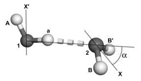
Figure 2: Water dimer in its optimal configuration. See Table 4 for structure details.

A close analysis of the structure and potential energy curves (PECs) of the water dimer is of special interest since most anomalies in the interaction potential would be easiest to recognize in this simple system. Figure 2 shows the water dimer in its optimal configuration while Table 4 presents a comparison between the results predicted by our potential, the NCC[55] and ASP-W4[57, 58] potentials, and ab initio MP2/aug-cc-pVTZ results. The ASP-W4 and NCC calculations were performed using Orient 3.2[81], while the Gaussian 98[82] package was used for the ab initio calculations. SCME and ASP-W4 give rather similar results. The main errors observed for the latter are the 0.06 Å overestimation of the r_OO distance (a problem that is also found on the larger clusters) and the buckling of the hydrogen bond in the wrong direction. The NCC potential also shows an overestimation of the O-O distance and a rather large overestimation of the wagging angle of the acceptor monomer (1,2,X). Finally, the largest error shown by SCME ocurrs for the (1,2,X) angle which is underestimated by about 9^∘.

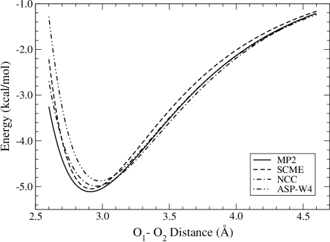
Figure 3: Comparison of the potential energy curves for (H₂O)₂ calculated with our model potential and several other methods. The O-O distance was varied while the rest of the structure was kept at its optimal configuration. See Figure 2 for structure details.

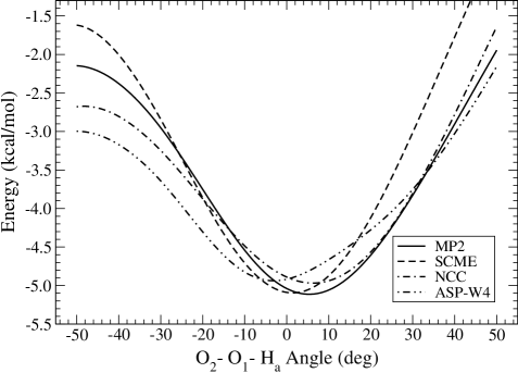
Figure 4: Comparison of the potential energy curves for (H₂O)₂ calculated with our model potential and several other methods. The hydrogen bond angle was varied while the rest of the structure was kept at its optimal configuration. See Figure 2 for structure details.

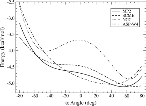
Figure 5: Comparison of the potential energy curves for (H₂O)₂ calculated with our model potential and several other methods. The acceptor monomer wagging angle was varied while the rest of the structure was kept at its optimal configuration. See Figure 2 for structure details.

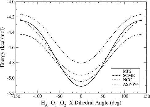
Figure 6: Comparison of potential energy curves for (H₂O)₂ calculated with our model potential and several other methods. The free hydrogen in the donor monomer was rotated around the hydrogen bond while the rest of the structure was kept at its optimal configuration. See Figure 2 for structure details.

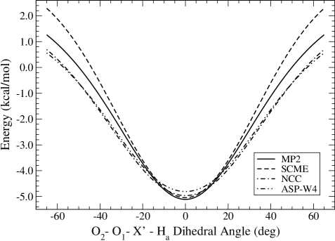
Figure 7: Comparison of potential energy curves for (H₂O)₂ calculated with our model potential and several other methods. The acceptor monomer was rotated around the donor monomer while the rest of the structure was kept at its optimal configuration. See Figure 2 for structure details.

Figures 3-7 show the PECs for the deformation of the water dimer along five coordinates of special interest. These curves were obtained by varying a given coordinate while keeping the rest of the structure fixed at the optimal MP2 values. Figure 3 shows that, in the long-range regions (r${}_{OO}>$ 3.2 Å ), these potentials are essentially equivalent, a consequence of the similarity between the electrostatic+induction components used by each of them. Some differences appear for the short-range interaction region, although in general they are well within the expected accuracy of the models. The most important exceptions to this observation occur for the variation of the hydrogen bond angle and the acceptor monomer wagging angles (Figures 4 and 5).

In the first case (Figure 4), the NCC and SCME potentials behave similarly in the minimum region, with the NCC potential showing the best overall agreement with the ab initio results. The deviation shown by ASP-W4 is small but significant since the buckling of the hydrogen bond is in the opposite direction to that predicted by the ab initio calculations. For larger deformations of the angle, however, the potentials show some notorious differences. For example, the predicted barrier for the switching of the hydrogen bond from H${}_{\text{a}}$ to H${}_{\text{A}}$ varies by 1.5 kcal/mol. This is especially true for ASP-W4, which underestimates the barrier by almost 1 kcal/mol. For the deformation in the opposite direction, the largest deviation is observed for the SCME potential, which overestimates the repulsion between the lone electron pairs of each monomer.

Figure 5 shows the variation of the acceptor monomer wagging angle. For this distortion, the best behavior is observed for our new potential, which correctly reproduces the shoulder corresponding to the transference of the hydrogen bond from one lone electron pair to the other. In the case of the NCC potential this shoulder is completely missing, predicting an equilibrium angle that is smaller than the one predicted by the MP2 results. The most striking feature is the barrier predicted by the ASP-W4 potential. This barrier and the minimum observed around -45^∘ are the result of the restriction of the O-O distance to a value smaller than the optimal for ASP-W4. When the PEC is calculated at a longer distance, these features disappear.

Since the only non-spherically symmetric contributions to the SCME potential energy arise from the electrostatic+induction terms, the differences observed between the ab initio and SCME results must be associated with these terms. Moreover, since the multipole moments used in the model potential are essentially identical to those obtained at MP2 level, we conclude that the origin of the differences must lie in either the damping function used for the electric field and its gradients, or in the quality of the induction approximation used.

3.2 The (H₂O)_n Clusters with $n=$3 to 6

3.2.1 Ring Clusters

The next important test of the potential function comes from the comparison of the predicted structures of the small ring clusters to those obtained with ab initio methods. Tables 5-8 present these results and Figure 8 explains the labels used. We have divided the analysis of the results into different types of coordinates, i.e., O-O distances, hydrogen-bond angles (1,a,2), O-framework dihedrals (1,2,3,4), free hydrogen-O-framework dihedrals (A,1,2,3) and free hydrogen-free hydrogen dihedrals (A,1,2,B).

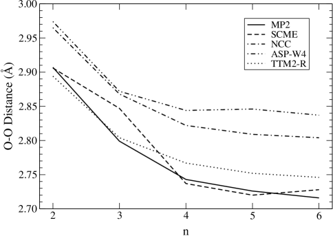
Figure 9: Comparison of the average O-O distance for the (H₂O)_n=2-6 clusters calculated with our model potential and several other methods.

The SCME potential gives good results for the O-O distance, with a mean absolute deviation with respect to the MP2 values of only 0.02 Å. This is to be compared with the 0.08 and 0.10 Å deviations shown by NCC and ASP-W4, respectively. This good agreement can be seen in Figure 9, which compares the average O-O distance for each cluster calculated with the methods mentioned above. It is clear that, with the exception of the trimer, the SCME potential provides an accurate description of the variation in the O-O distance, while NCC and ASP-W4 largely give an overestimate.

Angles between hydrogen-bonds are best described by the NCC potential with a mean absolute deviation of 2^∘. The SCME and ASP-W4 potentials give slightly larger deviations of 5^∘ and 6^∘, respectively. Perhaps the most striking result is the rather large error (about 11^∘) shown by the ASP-W4 potential for the water hexamer. The SCME potential provides good estimates for the three different types of dihedral angles studied. In the case of the O-framework dihedral angles we obtain significantly lower deviations than those obtained with the other potentials. This is especially true in the case of NCC, which shows large errors in those dihedrals for all clusters. Moreover, although both ASP-W4 and NCC show similar mean deviations, the former shows a very large (about 25^∘) error in the case of the hexamer. For the other dihedrals our results are similar to those obtained with ASP-W4 and significantly better than the NCC results.

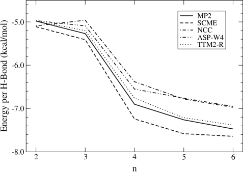
Figure 10: Comparison of the interaction energy per hydrogen bond for the (H₂O)_n=2-6 clusters calculated with our model potential and several other methods. MP2 and TTM2-R energies taken from Refs. [83] and [59], respectively.

In Table 9 we present the interaction energy for the (H₂O)_n=3-6 clusters at their optimized geometry. Also included for comparison are results for the water dimer. As in the previous section, we compare our results to those obtained with the ASP-W4 and NCC model potentials. We also include ab initio MP2/CBS results[83] and TTM2-R[59, 60] results taken from the literature. The mean absolute deviation between our potential and the MP2 results is only 0.9 kcal/mol, about half of the deviation observed for both NCC and ASP-W4 (1.6 kcal/mol). It is, however, larger than the one observed for the TTM2-R potential (0.3 kcal/mol) [59]. Figure 10 shows the variation of the interaction energy per hydrogen bond with the size of the cluster. Both NCC and ASP-W4 underestimate the interaction energy, with this underestimation increasing for the larger clusters, while TTM2-R does an excellent job in predicting the interaction energies of these clusters. Our new potential consistently overestimates the interaction energy by about 0.2 kcal/mol per hydrogen bond. This deviation, probably related to the functional form used for the repulsion component, is also found for the energies of some isomers of the water hexamer (see Section 3.2.2).

For all the structural parameters described above, the largest differences between the SCME and MP2 results occur for the water trimer, a cluster that poses a special challenge for our potential. For example, if only (H₂O)_n=4-6 are considered, the deviation of the SCME O-O distances from the ab initio results is only 0.008 Å. Similarly, the free hydrogen-free hydrogen dihedral angles show a mean deviation of almost 15^∘ for the trimer, but are only 6^∘ for the hexamer. These discrepancies arise from a mixture of problems that we believe originate from the repulsion component. First, (H₂O)₃ has a strained structure that takes the potential into regions where the dimer-based parametrization of the two-body part of the repulsion is less accurate. Second, for the parametrization of the density-dependent repulsion term, we assumed that the $B$ parameter increases monotonically with the local density at each of the monomers. This approximation is not adequate in the case of the ring structure of the trimer. There is a subtle balance between the O-O distances and the dihedral angles that is controlled by the strength of the repulsion between the monomers.

3.2.2 The Cage, Prism, Book and Ring Isomers of (H₂O)₆

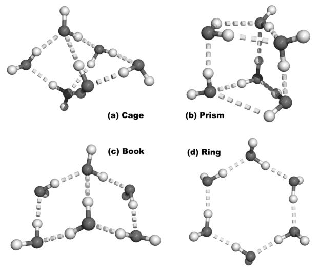
Figure 11: Structure of the cage, prism, book and ring isomers of (H₂O)₆.

Of all the stable conformations of (H₂O)₆, the so-called prism, cage, book and ring isomers (Figure 11) have become a benchmark to test new water potentials. The near degeneracy and difference in structure make them ideal to discover imbalances and problems in model interaction potentials. Table 10 presents a comparison of the theoretical interaction energies of these clusters calculated with the SCME potential to the same methods discussed in the previous section, and in addition to more recent $\Delta$CCSD(T) results computed by adding the MP2-CCSD(T) energy difference at the triple-zeta basis set level to the complete basis set (CBS) MP2 results[44]. The TTM2-R potential provides the best results with a mean absolute deviation of 0.5 kcal/mol. The ASP-W4 and SCME potentials have similar deviations ($\sim$1.6 kcal/mol), while for NCC the results are slightly less accurate (deviation $\sim$2.0 kcal/mol). The ring isomer is predicted as the least stable of all the structures by all the potentials used, in agreement with the $\Delta$CCSD(T) results. The relative stability of the remaining isomers is less clear due to their very similar energies. Although the ASP-W4 and NCC potentials give the correct energetic ordering for the different isomers (i.e. $E_{prism}<E_{cage}<E_{book}<E_{ring}$), the book isomer is predicted to be too loosely bound relative to the prism and cage isomers when comparing with the $\Delta$CCSD(T) results. On the other hand, both the TTM2-R and SCME potentials give a dispersion of the energies in better agreement with the ab initio results. The errors observed for the SCME potential are consistent with the systematic overestimation of the binding energies discussed in the previous section. For each of the hexamer isomers, the error is $\sim$0.2 kcal/mol per hydrogen bond. If this systematic error is removed by applying a constant correction to each bond energy, the mean absolute deviation of the total energies predicted with our potential is only 0.4 kcal/mol.

3.3 Liquid Water

The SCME potential is intended to be applicable over a wide range of configurations of the molecules including those of liquid water, even though no information about liquid water was used in the development of the potential function. The properties of liquid water calculated with the SCME potential function therefore represent a prediction. Canonical molecular dynamics simulations were carried out at 298K using a cubic cell of 19.72 Å per side, containing 256 molecules. Four uncorrelated initial configurations were extracted from a previous classical force field simulation. The step used in the integration of the equations of motion was 2 fs. Each cell was equilibrated until the average of the total energy was observed to remain constant, after which statistics were collected for 400 ps. During the equilibration period, the temperature was reset to 298K every 50 fs by redistributing the translational and rotational velocities of all the molecules according to a Boltzmann distribution [84]. During the collection period, the temperature was kept constant at 298K by readjusting the velocity of single molecules every 50 fs. The computational time needed for a simulation of 500 time steps on a single core Intel Xeon 3.5 GHz processor was 20 min.

From the simulated trajectory, we generated the radial distribution functions (RDFs). Each run resulted in very similar distribution functions, thus confirming the independence of the final result from the initial configuration. Figures 12-14 show the O-O, O-H and H-H RDF curves, obtained by averaging the four runs performed. An O-O curve obtained from a systematic study of x-ray diffraction datasets[85] is also shown as well as O-H and H-H curves obtained from EPSR[86] and RMC[87] structure refinement of x-ray and neutron scattering experiments. The agreement between experiment and our theoretical results is rather good for each of the three RDF curves, especially in view of the fact that our potential function has in no way been adjusted to reproduce such data and considering that the experimental RDF curves contain uncertainties. Two main differences between our simulation and the experiments are a shift of the second peak in the O-O curve to shorter distances and more structured long-range regions predicted by our potential. For better comparison we should carry out quantum mechanical simulations rather than classical simulations since a significant softening of the structure may occur[88, 89, 90]. Indeed, in a recent series of path-integral simulations[90] it was found that the first peak of the O-O g(r) was lowered by about 0.4 compared to classical dynamics simulation, which corresponds closely with the discrepancy in peak height observed here in Figure 12.

The definition of the electric properties of a molecule embedded in a condensed phase is subject to ambiguity. The difficulty of arriving at meaningful values for these quantities by use of ab initio methods has been pointed out[91]. A recent theoretical estimate for ice gave significantly larger values than previous estimates, ca. 3.1 Debye[67]. Our calculations of liquid water with the SCME potential give an average molecular moment of 2.96 $\pm$ 0.26 Debye (obtained by averaging over all the cells used and over all the molecules in each cell). This value is in good agreement with a density functional theory estimate of 2.95 Debye[92]. The TTM2-R model potential, on the other hand, gives a dipole moment of 2.65 Debye[59], a significantly lower value.

Finally, the average potential energy of the liquid predicted by the SCME potential and classical trajectory calculations is -10.8 kcal/mol per molecule. The best experimental estimate is -9.86 kcal/mol per molecule[93] but there quantum mechanical, zero point energy effects are included. In order to obtain a closer comparison with experiments, one should employ a quantum mechanical simulation to properly take into account zero point energy effects since the SCME is derived to reproduce the potential energy surface without any quantum corrections. Model potentials parametrized to reproduce experimental properties give results that are closer to experiment. For example, TIP4P predicts an average energy of -9.83 kcal/mol per molecule[59], while the closely related TIP4P-FQ potential gives a value of -9.92 kcal/mol per molecule[94].

3.4 Ice

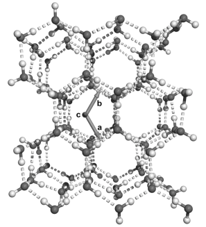
Figure 15: Typical orthorombic cell used for the simulation of (proton disordered) ice Ih.

One of our main interests in developing this new potential function is to use it for simulations of ice growth. The present study is limited to the most common phase of crystalline ice, i.e. ice Ih. We simulated a crystal sample containing 96 water molecules, built from $3\times 2\times 2$ repetitions of a generic 8-molecule orthogonal cell[95]. Since ice Ih is proton-disordered, a Monte Carlo algorithm was used to generate ten different cells that comply with the ice rules and have null overall dipole moments. Figure 15 shows a typical example of the cells used in this work. As in the case of liquid water, the properties discussed in this section were averaged over the different cells used. Table 11 presents the energy, conformational parameters and electric properties of ice Ih. The values obtained with the SCME potential are compared with experimental, density functional and model potential results when available.

The many-body component of the repulsion energy in the SCME interaction potential function was adjusted to fit both the MP2 dimer potential energy surface and the experimental cohesive energy and lattice parameters of ice[96], after the cohesive energy had been corrected to remove thermal and zero-point energy effects. As a result, the cohesive energy for ice is better reproduced by SCME than for example the PW91 density functional[97] and several pairwise additive and polarizable potentials. SCME also gives good agreement with the experimental lattice parameters, the calculated values being only slightly smaller (by $\sim$0.03 Å). This small error, nevertheless, makes the density slightly too high. The value predicted by SCME is, however, a significant improvement over simple pair potentials such as TIP4P.

The average O-O distance and the bulk modulus are useful measures of the quality of the potential since these were not included in the fitting of the repulsive component. The value predicted for the former is 2.742 Å, only 0.01 Å smaller than the experimental value. This small overbinding is related to the underestimation of the lattice parameters discussed above. In the case of the bulk modulus, the SCME value is better than that obtained with DFT and significantly better than those from other model potentials. It is, however, somewhat larger than the experimentally determined value, making the potential slightly too stiff.

Also included in Table 11 is the dipole moment of the monomer embedded in the ice Ih lattice. As discussed in the previous section, the definition of the dipole moment in ice is ambiguous and both the experimental[98] and theoretical values present in the literature cover a rather wide range[91]. The multipole expansion on which the SCME potential is based gives a value that is larger than many previous estimates, even by as much as 0.5 Debye[99].

4 Conclusions

We have presented and tested a new model potential for the interaction between water molecules based on a single-center multipole expansion (SCME) up to and including hexadecapole and including both dipole and quadrupole polarizability. Since point charges are not included, it is possible in some cases to simply truncate the potential at long range and thereby avoid the evaluation of Ewald sums. This reduces the computational effort significantly and while this potential function has many terms and a detailed description of the electrostatics through a multipole expansion, it is still computationally efficient and applicable to large and complex systems. The electrostatic, induction and dispersion components of the energy are obtained from ab initio and experimental molecular properties of the monomer, while the repulsive part of the potential was adjusted to reproduce ab initio results for the dimer and the small ring-shaped clusters as well as the experimentally determined cohesive energy of ice Ih. Since the electrostatics are evaluated including both dipole and quadrupole polarization through a self-consistency procedure, the potential should be transferable to a wide range of systems, well beyond the few that were used in the parametrization.

Our test results showed that, in general, the SCME potential is equally or even more accurate than other sophisticated model potentials currently available. The binding energy and structure of small clusters are in quite good agreement with the best available theoretical estimates. Some of the more subtle features of the potential energy surface of the water dimer are well reproduced. With the exception of the water trimer, the interaction energy for the ring clusters are in excellent agreement with MP2/CBS results. For other clusters, such as the most stable isomers of the water hexamer, the absolute values of the interaction energy is less accurate, but the relative values for the different conformers are in good agreement with best estimates, such as CCSD(T) calculations. In the case of the condensed phases, the energy and structural parameters are in excellent agreement with experiment. SCME reproduces the radial distribution function curves of the liquid and the lattice structure of ice Ih quite well.

The systematic deviations observed for the (H₂O)_n=2-6 clusters show that there is still room for improvement. In particular, the structure obtained for the water trimer could be improved. We believe these problems originate mostly from the lack of flexibility of the functional form used for the repulsive exchange interaction. Other sources of error can probably be found in the damping function used for the electric fields and possibly also in the values used for the multipole moments and polarizabilities. However, the functional form used in SCME includes the essential physics of the problem and it should be possible to obtain a highly accurate parametrization of the water interaction with this form using a more systematic parametrization from high level ab initio calculations.

Table 1: Multipole moments of the water molecule used in the calculation of the electrostatic and induction components of the interaction energy. All values in atomic units. All moments defined with respect to the center of mass. Molecular orientation as shown in Figure 1.

• Multipole Moment	Component
  Dipolea	$\mu_{z}$	-0.72981
  Quadrupoleb	$\Theta_{xx}$	1.95532
  	$\Theta_{yy}$	-1.85867
  	$\Theta_{zz}$	-0.09665
  Octupolec	$\Omega_{xxz}$	-3.27190
  	$\Omega_{yyz}$	1.36606
  	$\Omega_{zzz}$	1.90585
  Hexadecapolec	$\Phi_{xxxx}$	-0.94903
  	$\Phi_{xxyy}$	-3.38490
  	$\Phi_{xxzz}$	4.33393
  	$\Phi_{yyyy}$	4.09835
  	$\Phi_{yyzz}$	-0.71345
  	$\Phi_{zzzz}$	-3.62048

  
  

  ^a From Ref. [73]
  ^b From Ref. [74]
  ^c From Ref. [67]

Table 2: Polarizabilities used in the calculation of the induction component of the interaction energy. All values in atomic units. All moments defined with respect to the center of mass. Molecular orientation as shown in Figure 1.

• Polarizability	Component
  Dipole-Dipolea	$\alpha_{xx}$	10.31146
  	$\alpha_{yy}$	9.54890
  	$\alpha_{zz}$	9.90656
  Dipole-Quadrupolea	$A_{x,xz}$	-8.42037
  	$A_{y,yz}$	-1.33400
  	$A_{z,xx}$	-2.91254
  	$A_{z,yy}$	4.72407
  	$A_{z,zz}$	-1.81153
  Quadrupole-Quadrupolea	$C_{xx,xx}$	12.11907
  	$C_{xx,yy}$	-6.95326
  	$C_{xx,zz}$	-5.16582
  	$C_{xy,xy}$	7.86225
  	$C_{xz,xz}$	11.98862
  	$C_{yy,yy}$	11.24741
  	$C_{yy,zz}$	-4.29415
  	$C_{yz,yz}$	6.77226
  	$C_{zz,zz}$	9.45997

  
  

  ^a These values correspond to a translational transformation of those reported in Ref. [57].

Table 3: Other parameters used in the calculation of the interaction energy. All values in atomic units.

• Component	Parameter
  Damping	$\tau_{d}$	2.32837906
  Electrostatic+Induction	$r_{h_{1}}$	9.44863332
  	$r_{l_{2}}$	17.00753997
  	$r_{h_{2}}$	20.78699330
  Dispersion a	$C_{6}$	46.44309964
  	$C_{8}$	1141.70326668
  	$C_{10}$	33441.11892923
  Repulsion	$A$	1857.45898793
  	$C$	1.68708507 $\times 10^{6}$
  	$b$	1.44350000
  	$c$	1.83402715
  	$d$	0.35278471
  	$a_{0}$	1.02508535 $\times 10^{-1}$
  	$a_{1}$	-1.72461186 $\times 10^{-4}$
  	$a_{2}$	1.02195556 $\times 10^{-7}$
  	$a_{3}$	-2.60877107 $\times 10^{-11}$
  	$a_{4}$	3.06054306 $\times 10^{-15}$
  	$a_{5}$	-1.32901339 $\times 10^{-19}$

  
  

  ^aFrom Ref. [78]

Table 4: Comparison of the optimal structure of the water dimer obtained with different methods. See Figure 2 for a definition of each structure coordinate.

• Coordinate	Atoms	MP2	SCME	NCC	ASP-W4
  Distance [Å]	(1,2)	2.907	2.906	2.965	2.974
  Angle [deg]	(1,a,2)	171.57	175.42	179.49	-176.95
  	(1,2,X)	123.09	113.99	152.77	123.03
  Dihedral [deg]	(A,1,2,B)	122.96	125.27	109.50	122.98

Table 5: Comparison of the optimal structure of the water trimer obtained with different methods. See Figure 8 for a definition of each structure coordinate.

• Coordinate	Atoms	MP2	SCME	NCC	ASP-W4
  Distance [Å]	(1,2)	2.799	2.840	2.865	2.868
  	(2,3)	2.798	2.843	2.868	2.865
  	(3,1)	2.800	2.858	2.871	2.884
  Angle [deg]	(1,a,2)	151.26	158.73	149.28	148.47
  	(2,b,3)	151.11	158.65	149.13	148.24
  	(3,c,1)	148.39	157.22	147.99	145.70
  Dihedral [deg]	(A,1,2,3)	-129.13	-114.08	-145.80	-120.67
  	(B,2,3,1)	118.38	110.63	128.46	119.20
  	(C,3,1,2)	-122.71	-111.14	-140.01	-121.92
  	(A,1,2,B)	129.49	148.63	114.99	144.04
  	(B,2,3,C)	-133.86	-151.90	-130.35	-135.34
  	(C,3,1,A)	-21.87	-14.78	-36.55	-27.72

Table 6: Comparison of the optimal structure of the water tetramer obtained with different methods. See Figure 8 for a definition of each structure coordinate.

• Coordinate	Atoms	MP2	SCME	NCC	ASP-W4
  Distance [Å]	(1,2)	2.743	2.737	2.822	2.844
  Angle [deg]	(1,a,2)	167.64	173.27	165.69	163.69
  Dihedral [deg]	(4,1,2,3)	-0.48	1.35	-9.90	1.75
  	(A,1,2,3)	123.45	118.24	128.17	123.71
  	(A,1,2,B)	-123.69	-134.93	-113.86	-132.36

Table 7: Comparison of the optimal structure of the water pentamer obtained with different methods. See Figure 8 for a definition of each structure coordinate.

• Coordinate	Atoms	MP2	SCME	NCC	ASP-W4
  Distance [Å]	(1,2)	2.722	2.717	2.806	2.839
  	(2,3)	2.725	2.719	2.809	2.843
  	(3,4)	2.734	2.729	2.815	2.869
  	(4,5)	2.726	2.716	2.810	2.840
  	(5,1)	2.723	2.717	2.807	2.838
  Angle [deg]	(1,a,2)	175.91	177.41	173.57	168.74
  	(2,b,3)	176.77	178.11	174.14	169.26
  	(3,c,4)	173.01	176.99	172.94	174.42
  	(4,d,5)	176.65	178.16	175.72	169.12
  	(5,e,1)	175.72	177.07	173.08	168.69
  Dihedral [deg]	(1,2,3,4)	15.23	10.69	19.02	2.84
  	(2,3,4,5)	-9.19	-11.36	-4.26	-6.29
  	(3,4,5,1)	-0.28	7.70	-12.10	7.43
  	(4,5,1,2)	9.66	-1.07	23.79	-5.66
  	(5,1,2,3)	-15.46	-5.99	-26.54	1.70
  	(A,1,2,3)	114.41	115.80	116.96	124.04
  	(B,2,3,4)	-113.02	-111.00	-123.06	-119.48
  	(C,3,4,5)	117.47	107.62	139.54	117.55
  	(D,4,5,1)	136.05	134.38	159.73	127.55
  	(E,5,1,2)	-115.38	-119.66	-118.00	-126.55
  	(A,1,2,B)	-124.93	-129.72	-114.85	-126.16
  	(B,2,3,C)	124.95	136.35	106.87	125.84
  	(C,3,4,D)	-8.70	-9.41	-27.07	9.43
  	(D,4,5,E)	-106.47	-113.30	-72.81	-123.28
  	(E,5,1,A)	123.43	126.14	112.86	124.16

Table 8: Comparison of the optimal structure of the water hexamer obtained with different methods. See Figure 8 for a definition of each structure coordinate.

• Coordinate	Atoms	MP2	SCME	NCC	ASP-W4
  Distance [Å]	(1,2)	2.716	2.728	2.804	2.837
  Angle [deg]	(1,a,2)	178.73	174.80	176.07	167.16
  Dihedral [deg]	(1,2,3,4)	20.63	12.90	35.16	-4.90
  	(A,1,2,3)	112.60	113.61	114.05	126.92
  	(A,1,2,B)	-120.40	-125.92	-106.97	-120.30

Table 9: Comparison of the interaction energy of the ring shaped (H₂O)_n clusters obtained with different methods. All values in kcal/mol.

• n	MP2/CBSa	SCME	NCC	ASP-W4	TTM2-Rb
  2	-4.98	-5.11	-5.09	-4.97	-4.98
  3	-15.8	-16.22	-14.88	-15.28	-15.59
  4	-27.6	-28.95	-25.51	-26.19	-27.03
  5	-36.3	-37.88	-33.92	-33.82	-36.05
  6	-44.8	-45.86	-41.80	-41.68	-44.28

  
  

  ^a From Ref. [83]
  ^b From Ref. [59]

Table 10: Comparison of the interaction energy of the cage, prism, book and ring isomers of (H₂O)₆ obtained with different methods. All values in kcal/mol.

• Conformation	$\Delta$CCSD(T)/CBSa	SCME	NCC	ASP-W4	TTM2-Rb
  Prism	-46.2	-47.56	-44.78	-45.87	-45.11
  Cage	-45.9	-47.64	-44.41	-44.74	-45.67
  Book	-45.5	-47.77	-43.11	-43.61	-45.14
  Ring	-44.5	-45.86	-41.80	-41.68	-44.28

  
  

  ^a From Ref. [44]
  ^b From Ref. [59]

Table 11: Comparison between some experimental properties of ice Ih at 0K and those obtained with ab initio methods, the SCME model potential and other potentials commonly used: $\Delta E_{Lattice}$ (lattice energy, in eV/molec), $\langle r_{OO}\rangle$ (average O-O distance, in Å), $a$, $b$, $c$ (lattice parameters for the eight-molecule orthorhombic cell, in Å), $\rho$ (density, in g/cm³), $V_{molec}$ (molecular volume, in ų/molec), $K$ (bulk modulus, in MPa), $\mu_{molec}$ (molecular dipole moment, in Debye).

Property	Exp.a	PW91b	SCME	TIP4Pc	RWK2d	DCe	TTM2-Rf
$\Delta E_{Lattice}$	-0.6110	-0.55g	-0.6109$\pm$0.0049	-0.634	-0.555	-0.550	-.6370
$\langle r_{OO}\rangle$	2.751	2.70	2.742$\pm$0.004	2.683		2.738
$a$	4.4969	4.41	4.470$\pm$0.025				4.478
$b$	7.7889	7.63	7.747$\pm$0.052				7.756
$c$	7.3211	7.20	7.287$\pm$0.029				7.314
$\rho$	0.933	0.989, 0.954g	0.948$\pm$0.004	1.009	0.942	0.960	0.942
$V_{molec}$	32.05	30.3, 31.35g	31.55$\pm$0.15	29.62	31.73	31.14	31.75
$K$	10.9	13.5	11.4$\pm$0.3	16.6	18.0
$\mu_{molec}$	2.90	2.8	3.50$\pm$0.07	2.18		3.02	2.86h

^a All values from Ref. [11] with the exception of the bulk modulus, taken from Ref. [100].
^b All values from Ref. [101] unless indicated.
^c All values from Ref. [56] with the exception of the bulk modulus, taken from Ref. [102].
^d From Ref. [103].
^e From Ref. [56].
^f From Ref. [59].
^g From Ref. [97].
^h Calculated at 100K.

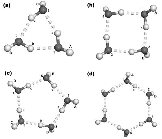
Figure 8: Optimal conformations of the (H₂O)_n=3-6 clusters. See Tables 5-8 for structure details.

Figure 12: Comparison of experimental[85] and theoretical O-O radial distribution functions of liquid water at 298K.

Figure 13: Comparison of experimental[86, 87] and theoretical O-H radial distribution functions of liquid water at 298K.

Figure 14: Comparison of experimental[86, 87] and theoretical H-H radial distribution functions of liquid water at 298K.

References

- [1] Ball P, Life’s matrix: a biography of water, (University of California Press2001)
- [2] Cheung M S, García A E and Onuchic J N, 2002 Proc. Natl. Acad. Sci. (USA), 99 685
- [3] Li I T and Walker G C, 2011 Pro. Natl. Acad. Sci. (USA), 108 16527–16532
- [4] Snyder P W, Mecinović J, Moustakas D T, Thomas III S W, Harder M, Mack E T, Lockett M R, Héroux A, Sherman W and Whitesides G M, 2011 Proc. Natl. Acad. Sci. (USA), 108 17889–17894
- [5] Grossman M, Born B, Heyden M, Tworowski D, Fields G B, Sagi I and Havenith M, 2011 Nature Struct. & Mol. Bio., 18 1102–1108
- [6] Speedy R J and Angell C A, 1976 The Journal of Chemical Physics, 65(3) 851–858
- [7] Poole P H, Sciortino F, Essmann U and Stanley H E, 1992 Nature, 360(6402) 324–328
- [8] Debenedetti P G, 2003 J. Phys: Cond. Matt., 15(45) R1669
- [9] Pierrehumbert R T. In Clark P U, Webb R S and Keigwin L D (eds.) Mechanisms of Global Change at Millennial Timescales, volume 112 of Geophys. Monogr. Ser., (American Geophysical Union, Washington DC1999)
- [10] Held I M and Soden B J, 2000 Annu. Rev. Energ. Environ., 25 441
- [11] Petrenko V F and Withworth R W, Physics of Ice, (Oxford University Press1999)
- [12] Smith J, Stone R and Fahrenkamp-Uppenbrink J, 2002 Science, 297 1489
- [13] Paterson W S B, The Physics of Glaciers, (Pergamon/Elsevier Science, Oxford1994)
- [14] Pruppacher H R and Klett J D, Microphysics of Clouds and Precipitation, (Kluwer Academic Publishers, Dordrecht1997)
- [15] Ehrenfreund P, Composition of comets and interstellar dust. In Rickman H (ed.) Highlights of Astronomy, volume 12 of IAU Symposia, p. 229, (Astronomical Soc. Pacific, San Fransisco2002)
- [16] Ehrenfreund P and Schutte W A, Infrared observations of interstellar ices. In Minh Y C and van Dishoeck E F (eds.) Astrochemistry: From Molecular Clouds to Planetary Systems, volume 197 of IAU Symposia, p. 135, (Astronomical Soc. Pacific, San Fransisco2000)
- [17] Caro G M M, Meierhenrich U J, Schutte W A, Barbier B, Segovia A A, Rosenbauer H, Thiemann W H P, Brack A and Greenberg J M, 2002 Nature, 416 403
- [18] Burton E F and Oliver W F, 1935 Proc. R. Soc. Lon. A, 153 166
- [19] Mayer E and Brüggeller P, 1982 Nature, 298 715
- [20] McCammon D, Moseley S, Mather J, Musholzky R, Fiorini E and Niinikoski T, 1985 Nature, 314 7
- [21] Jenniskens P and Blake D F, 1994 Science, 265 753
- [22] Hallbrucker A, Mayer E and Johari G P, 1989 J. Phys. Chem., 93 4986
- [23] Dash J G, Fu H and Wettlaufer J S, 1995 Reports on Progress in Physics, 58 115
- [24] Furukawa Y and Nada H, 1997 J. Phys. Chem. B, 101 6167
- [25] Kroes G J, 1992 Surf. Sci., 275 365
- [26] Morgenstern M, Müller J, Michely T and Comsa G, 1997 Z. Phys. Chem., 198 43
- [27] Materer N, Starke U, Barbieri A, Hove M A V, Somorjai G A, Kroes G J and Minot C, 1997 Surf. Sci., 381 190
- [28] Braun J, Glebov A, Graham A P, Menzel A and Toennies J P, 1998 Phys. Rev. Lett., 80 2638
- [29] Kryachko E S and Ludeña E V, Energy Density Functional Theory of Many-Electron Systems, (Kluwer Academic Publishers, Dordrecht1990)
- [30] March N H, Electron Correlation in Molecules and Condensed Phases. Physics of Solids and Liquids, (Plenum Press, New York1996)
- [31] Frenkel D and Smit B, Understanding Molecular Simulation, (Academic Press, San Diego2002)
- [32] Stone A J, The Theory of Intermolecular Forces, pp. 74–75, (Clarendon Press, Oxford1996)
- [33] Xantheas S S, 1995 J. Chem. Phys., 102 4505
- [34] Bene J E D, Person W B and Szczepaniak K, 1995 J. Phys. Chem., 99 10705
- [35] Sprik M, Hutter J and Parrinello M, 1996 J. Chem. Phys., 105 1142
- [36] Grossman J C, Schwegler E, Draeger E W, Gygi F and Galli G, 2004 J. Chem. Phys., 120 300
- [37] Ireta J, Neugebauer J and Scheffler M, 2004 J. Phys. Chem. A, 108(26) 5692–5698
- [38] Santra B, Michaelides A and Scheffler M, 2007 J. Chem. Phys., 127 184104
- [39] Pérez-Jordá J M and Becke A D, 1995 Chem. Phys. Lett., 233 134
- [40] van Mourik T and Gdanitz R J, 2002 J. Chem. Phys., 116 9620
- [41] Dion M, Rydberg H, Schröder E, Langreth D C and Lundqvist B I, 2004 Phys. Rev. Lett., 92 246401
- [42] Vydrov O A and Voorhis T V, 2009 Phys. Rev. Lett., 103 63004
- [43] Lee K, Murray E D, Kong L, Lundqvist B I and Langreth D C, 2010 Phys. Rev. B, 82 081101
- [44] Klimeš J, Bowler D R and Michaelides A, 2010 J. Phys.: Cond. Matter, 22 022201
- [45] Wallqvist A and Mountain R D, Molecular models of water: Derivation and description. volume 13 of Reviews in Computational Chemistry, p. 183, (Wiley-VCH, New York1999)
- [46] Vega C and Abascal J L F, 2011 Phys. Chem. Chem. Phys., 13 19663–19688
- [47] Berendsen H J C, Grigera J R and Straatsma T, 1987 J. Phys. Chem., 87 6269
- [48] Jorgensen W L, Chandrasekhar J, Madura J D, Impey R W and Klein M L, 1983 J. Chem. Phys., 79 926
- [49] Horn H W, Swope W C, Pitera J W, Madura J D, Dick T J, Hura G L and Head-Gordon T, 2004 J. Chem. Phys., 120 9665
- [50] Abascal J L F and Vega C, 2005 J. Chem. Phys., 123 234505
- [51] Pedulla J M and Jordan K D, 1998 Chem. Phys., 239 593
- [52] Mhin B J, Kim J S, Lee S and Kim K S, 1993 J. Chem. Phys., 100 4484
- [53] Wales D J and Hodges M P, 1998 Chem. Phys. Lett., 286 65
- [54] Dang L X and Chang T M, 1997 J. Chem. Phys., 106 8149
- [55] Niesar U, Corongiu G, Clementi E, Kneller G R and Bhattacharya D K, 1990 J. Phys. Chem., 94 7949
- [56] Dong S, Wang Y and Li J, 2001 Chem. Phys., 270 309
- [57] Millot C and Stone A J, 1992 Mol. Phys., 77 439
- [58] Millot C, Soetens J C, Costa M T C M, Hodges M P and Stone A J, 1998 J. Phys. Chem. A, 102 754
- [59] Burnham C J and Xantheas S S, 2002 J. Chem. Phys., 116 1500
- [60] Burnham C J and Xantheas S S, 2002 J. Chem. Phys., 116 5115
- [61] Fanourgakis G S and Xantheas S S, 2008 J. Chem. Phys., 128 074506
- [62] Frenkel D and Smit B, Understanding Molecular Simulation, pp. 292–306, (Academic Press, San Diego2002)
- [63] Ewald P, 1921 Ann. Phys., 64 253
- [64] Allen M P and Tildesley D J, Computer Simulations of Liquids, pp. 155–162, (Clarendon Press, Oxford1987)
- [65] Liu Y and Ichiye T, 1996 J. Phys. Chem., 100 2723
- [66] Barnes P, Finney J L, Nicholas J D and Quinn J E, 1979 Nature, 282 459
- [67] Batista E R, Xantheas S S and Jónsson H, 1998 J. Chem. Phys., 109 4546
- [68] Batista E R, Xantheas S S and Jónsson H, 2000 J. Chem. Phys., 112 3285
- [69] Stone A J, The Theory of Intermolecular Forces, pp. 50–63,79–104, (Clarendon Press, Oxford1996)
- [70] Ahlrichs R, Penco P and Scoles G, 1977 Chem. Phys., 19 119
- [71] Stone A J, The Theory of Intermolecular Forces, p. 118, (Clarendon Press, Oxford1996)
- [72] Stone A J, The Theory of Intermolecular Forces, (Clarendon Press, Oxford1996)
- [73] Dyke T and Muenter J, 1973 J. Chem. Phys., 59 3125
- [74] Verhoeven J and Dymanus A, 1970 J. Chem. Phys., 52 3222
- [75] Gray C G and Gubbins K E, Theory of Molecular Fluids, (Clarendon Press, Oxford1984)
- [76] Stone A J, The Theory of Intermolecular Forces, pp. 94–96, (Clarendon Press, Oxford1996)
- [77] Tang K T and Toennies J P, 1984 J. Chem. Phys., 80 3726
- [78] Wormer P E S and Hettema H, 1992 J. Chem. Phys., 97 5592
- [79] Jónsson H, Levi A C and Weare J H, 1984 Phys. Rev. B, 30 2241
- [80] Jónsson H, Levi A C and Weare J H, 1984 Surf. Sci., 148 126
- [81] Stone A J, Dullweber A, Hodges M P, Popelier P and Wales D J, 1997. Orient 3.2j
- [82] Frisch M J et al., 1998. Gaussian 98, revision a.7
- [83] Burnham C J, Xantheas S S and Harrison R J, 2002 J. Chem. Phys., 116 1493
- [84] Andersen H, 1980 J. Chem. Phys., 72 2384
- [85] Skinner, L B and Huang, C and Schlesinger, D and Pettersson, L G M and Nilsson, A and Benmore, C J, 2013 J. Chem. Phys., 138 074506
- [86] Soper A K, 2007 J. Phys.: Cond. Matt., 19 335206
- [87] Wikfeldt K T, Leetmaa M, Ljungberg M P, Nilsson A and Pettersson L G M, 2009 J. Phys. Chem. B, 113 6246–6255
- [88] Kuharski R A and Rossky P J, 1984 Chem. Phys. Lett., 103 357
- [89] Lobaugh J and Voth G, 1997 J. Chem. Phys., 106 2400
- [90] Morrone J and Car R, 2008 Phys. Rev. Lett., 101 17801
- [91] Batista E R, Xantheas S S and Jónsson H, 1999 J. Chem. Phys., 111 6011
- [92] Silvestrelli P L and Parrinello M, 1999 J. Chem. Phys., 111 3572
- [93] Dorsey N E, Properties of Ordinary Water-Substance in All its Phases: water-vapor, water and all the ices, volume 81 of ACS Monograph Series, (Reinhold Publishing Corporation, New York1940)
- [94] Chialvo A A, Yezdimer E, Driesner T, Cummings P T and Simonson J M, 2000 Chem. Phys., 258 109
- [95] Petrenko V F and Withworth R W, Physics of Ice, p. 21, (Oxford University Press1999)
- [96] Petrenko V F and Withworth R W, Physics of Ice, pp. 29–30, (Oxford University Press1999)
- [97] Hamann D R, 1997 Phys. Rev. B, 55 R10157
- [98] Whalley E, 1978 J. Glaciology, 21 13
- [99] It should be noticed that the model presented in Ref.[67] used values for the polarization tensors calculated with respect to the Oxygen atom without transforming them to a center of mass origin. As a result, the average molecular dipole moment for ice Ih presented in this work is larger than the estimate reported in Ref. [67].
- [100] Hobbs P V, Ice Physics, (Clarendon Press, Oxford1974)
- [101] Jenkins S and Morrison I, 2001 J. Phys.: Condens. Matter, 13 9207
- [102] Batista E R, 1999 Development of a New Water-Water Interaction Potential and Application to Molecular Processes in Ice. Ph.D. thesis, University of Washington
- [103] Reimers J R, Watts R O and Klein M L, 1982 Chem. Phys., 64 95
-