Numerical Study of Quantized Vortex Interaction in Complex Ginzburg–Landau Equation on Bounded Domains

Abstract

In this paper, we study numerically quantized vortex dynamics and their interaction in the two-dimensional complex Ginzburg-Landau equation (CGLE) with a dimensionless parameter $\varepsilon>0$ on bounded domains under either Dirichlet or homogeneous Neumann boundary condition. We begin with a review of the reduced dynamical laws (RDLs) for time evolution of quantized vortex centers in CGLE and show how to solve these nonlinear ordinary differential equations numerically. Then we present efficient and accurate numerical methods for solving the CGLE on either a rectangular or a disk domain under either Dirichlet or homogeneous Neumann boundary condition. Based on these efficient and accurate numerical methods for CGLE and the RDLs, we explore rich and complicated quantized vortex dynamics and interaction of CGLE with different $\varepsilon$ and under different initial physical setups, including single vortex, vortex pair, vortex dipole and vortex lattice, compare them with those obtained from the corresponding RDLs, and identify the cases where the RDLs agree qualitatively and/or quantitatively as well as fail to agree with those from CGLE on vortex interaction. Finally, we also obtain numerically different patterns of the steady states for quantized vortex lattices in the CGLE dynamics on bounded domains.

1 Introduction

Vortices are those waves that possess phase singularities (topological defect) and rotational flows around the singular points. They arise in many physical areas of different scale and nature ranging from liquid crystals and superfluidity to non-equilibrium patterns and cosmic strings [17, 42]. Quantized vortices in the two dimension are those particle-like vortices, whose centers are the zero of the order parameter, possessing localized phase singularity with the topological charge (also called as winding number or index) being quantized. They have been widely observed in many different physical systems, such as the liquid helium, type-II superconductors, atomic gases and nonlinear optics [2, 5, 18, 34, 40]. Quantized vortices are key signatures of the superconductivity and superfluidity and their study is always one of the most important and fundamental problems since they were predicted by Lars Onsager in 1947 in connection with superfluid Helium.

In this paper, we consider the vortex dynamics and interactions in two dimensional complex Ginzburg–Landau equation (CGLE), which is one of the most studied nonlinear equations in physics community [3]. It has attracted ever more attention, because it can describe various phenomena ranging from nonlinear waves to second-order phase transitions, from superconductivity, superfluidity and Bose-Einstein condensation to liquid crystals and strings in field theory [3, 22, 23, 43]. The specific form of CGLE we study here reads as:

$$(\lambda_{\varepsilon}+i\beta)\partial_{t}\psi^{\varepsilon}({\bf x},t)=\Delta\psi^{\varepsilon}+\frac{1}{\varepsilon^{2}}(1-|\psi^{\varepsilon}|^{2})\psi^{\varepsilon},\qquad{\bf x}\in\mathcal{D},\quad t>0,$$ (1.1)

with initial condition

$$\psi^{\varepsilon}({\bf x},0)=\psi^{\varepsilon}_{0}({\bf x}),\qquad{\bf x}\in\overline{\mathcal{D}},$$ (1.2)

and under either Dirichlet boundary condition (BC)

$$\psi^{\varepsilon}({\bf x},t)=g({\bf x})=e^{i\omega({\bf x})},\qquad{\bf x}\in\partial\mathcal{D},\quad t\geq 0,$$ (1.3)

or homogeneous Neumann BC

$$\frac{\partial\psi^{\varepsilon}({\bf x},t)}{\partial\nu}=0,\qquad{\bf x}\in\partial\mathcal{D},\quad t\geq 0.$$ (1.4)

where $\mathcal{D}\subset\mathbb{R}^{2}$ is a bounded and simple connected domain in the paper, $t$ is time, ${\bf x}=(x,y)\in\mathbb{R}^{2}$ is the Cartesian coordinate vector, $\psi^{\varepsilon}:=\psi^{\varepsilon}({\bf x},t)$ is a complex-valued wave function (order parameter), $\omega$ is a given real-valued function, $\psi_{0}^{\varepsilon}$ and $g$ are given smooth and complex-valued functions satisfying the compatibility condition $\psi_{0}^{\varepsilon}({\bf x})=g({\bf x})$ for ${\bf x}\in\partial\mathcal{D}$, $\nu=(\nu_{1},\nu_{2})$ and $\nu_{\perp}=(-\nu_{2},\nu_{1})\in\mathbb{R}^{2}$ satisfying $|\nu|=\sqrt{\nu_{1}^{2}+\nu_{2}^{2}}=1$ are the outward normal and tangent vectors along $\partial\mathcal{D}$, respectively, $i=\sqrt{-1}$ is the unit imaginary number, $0<\varepsilon<1$ is a given dimensionless constant, and $\lambda_{\varepsilon}$, $\beta$ are two positive constants. Actually, the CGLE covers many different equations arise in various different physical fields. For example, when $\lambda_{\varepsilon}\neq 0$, $\beta=0$, it reduces to the Ginzburg-Landau equation (GLE) for modelling superconductivity. When $\lambda_{\varepsilon}=0$, $\beta=1$, the CGLE collapses to the nonlinear Schrödinger equation (NLSE) for modelling Bose-Einstein Condensation or superfluidity.

Denote the Ginzburg-Landau (GL) functional (‘energy’) as [15, 26, 37]

$$\mathcal{E}^{\varepsilon}(t):=\int_{\mathcal{D}}\left[\frac{1}{2}|\nabla\psi^{\varepsilon}|^{2}+\frac{1}{4\varepsilon^{2}}\left(1-|\psi^{\varepsilon}|^{2}\right)^{2}\right]d{\bf x}=\mathcal{E}_{\rm kin}^{\varepsilon}(t)+\mathcal{E}_{\rm int}^{\varepsilon}(t),\quad t\geq 0,$$ (1.5)

where the kinetic and interaction energies are defined as

$$\mathcal{E}_{\rm kin}^{\varepsilon}(t):=\frac{1}{2}\int_{\mathcal{D}}|\nabla\psi^{\varepsilon}|^{2}d\textbf{x},\quad\mathcal{E}_{\rm int}^{\varepsilon}(t):=\frac{1}{4\varepsilon^{2}}\int_{\mathcal{D}}\left(1-|\psi^{\varepsilon}|^{2}\right)^{2}d\textbf{x},\quad t\geq 0,$$

respectively. Then, it is easy to verify that the CGLE and GLE dissipate the energy, while the NLSE conserves the energy at all the time.

During the last several decades, constructions and analysis about the vortex solutions as well as studies of quantized vortex dynamics and interaction related with the CGLE (1.1) under different scalings have been extensively studied in the literatures. For the whole space case , i.e., $\mathcal{D}=\mathbb{R}^{2}$, Neu [40] studied dynamics and interaction of well-separated quantized vortices for GLE with $\lambda_{\varepsilon}=1$ and NLSE under scaling $\varepsilon=1$. He found numerically that quantized vortices with winding number $m=\pm 1$ are dynamically stable, and respectively, $|m|>1$ dynamically unstable in the GLE dynamics. Moreover, he found that vortices behave like point vortices in ideal fluid. Using asymptotic analysis, he derived the reduced dynamical laws (RDLs) which are sets of ordinary differential equations (ODEs) for governing the dynamics of the vortex centers to the leading order. Recently, Neu’s results were extented by Bethuel et al. to investigate the asymptotic behaviour of vortices as $\varepsilon\to 0$ in the GLE dynamics under the accelerating time scale $\lambda_{\varepsilon}=\frac{1}{\ln\frac{1}{\varepsilon}}$ [11, 12, 13] and in the NLSE dynamics [10]. The corresponding RDLs that govern the motion of the limiting vortices have also be derived.

Inspired by Neu’s work, many other papers have been dedicated to the study of the vortex states and dynamics for the GLE and NLSE with $0<\varepsilon<1$ on a bounded domain under different BCs. For the GLE case, Lin [34, 32, 33] considered the the dynamics of vortices in the asymptotic limit $\varepsilon\to 0$ under various scales of $\lambda_{\varepsilon}$ and with Dirichlet BC (1.3) or homogeneous Neumann (1.4). He derived the RDLs that govern the motion of these vortices and rigorously proved that vortices move with velocities of order $|\ln\varepsilon|^{-1}$ if $\lambda_{\varepsilon}=1$. Similar studies have also been conducted by E [21], Jerrard et al. [25], Jimbo et al. [29, 27] and Sandier et al. [44]. Unfortunately, all those RDLs are only valid up to the first time that the vortices collide or exit the domain and cannot describe the motion of multiple degree vortices. Recently, Serfaty [45] extended the RDLs for the dynamics of the vortices after collisions. For the NLSE case, Mironescu [39] and Lin [35] investigated stability of the vortices in NLSE with (1.3). Subsequently, Lin and Xin [37] studied the vortex dynamics on a bounded domain with either Dirichlet or Neumann BC, which was further investigated by Jerrard and Spirn [26]. In addition, Colliander and Jerrard [15, 16] studied the vortex structures and dynamics on a torus or under periodic BC. In these studies, RDLs were put forth to describe the asymptotic behaviour of the vortices as $\varepsilon\to 0$, which indicate that to the leading order the vortices move according to the Kirchhoff law in the bounded domain case. However, these RDLs cannot indicate radiation and/or sound propagations created by highly co-rotating or overlapping vortices. In fact, it remains as a very fascinating and fundamental open problem to understand the vortex-sound interaction [41], and how the sound waves modify the motion of vortices [22].

For the CGLE, under scaling $\lambda_{\varepsilon}\sim O(\frac{1}{\ln(1/\varepsilon)})$, Miot [38] studied the dynamics of vortices asymptotically as $\varepsilon\to 0$ in the whole plane case and Kurzke et al. [31] investigated that in the bounded domain case, the corresponding RDLs were derived to govern the motion of the limiting vortices in the whole plane and/or the bounded domain, respectively. Their results showed that the RDLs in the CGLE is actually a hybrid of RDL for GLE and that for NLSE. More recently, Serfaty and Tice [46] studied the vortex dynamics in a more complicated CGLE which involves electromagnetic field and pinning effect.

On the numerical aspects, finite element methods were proposed to investigate numerical solutions of GLE and related Ginzburg-Landau models for modelling superconductivity [20, 19, 30, 1, 14]. Recently, by proposing efficient and accurate numerical methods for solving the CGLE (1.1) in the whole space, Zhang et al. [49, 50] compared the dynamics of quantized vortices from the RDLs obtained by Neu with those obtained from the direct numerical simulation results from GLE and NLSE under different parameters and initial setups. Very recently, The second author designed some efficient and accurate numerical methods for studying vortex dynamics and interactions in the GLE and/or NLSE on bounded domains with either Dirichlet or Neumann BCs [7, 8]. These numerical methods can be extended and applied for studying the rich and complicated phenomena related to vortex dynamics and interaction in the CGLE (1.1) with either Dirichlet BC (1.3) or homogeneous Neumann BC (1.4) on bounded domains. The main purpose of this paper is organised as: (i). to present efficient and accurate numerical methods for solving the RDLs and the CGLE (1.1) on bounded domains under different BCs; (ii). to understand numerically how the boundary condition and geometry of the domain affect vortex dynamics and interction; (iii). to study numerically vortex interaction in the CGLE dynamics and/or compare them with those from the RDLs with different initial setups and parameter regimes; (iv). to identify cases where the reduced dynamical laws agree qualitatively and/or quantitatively as well as fail to agree with those from CGLE on vortex interaction.

The rest of the paper is organized as follows. In section 2, we briefly review the reduced dynamical laws of vortex interaction under the CGLE (1.1) with either Dirithlet or homogeneous Neumann BC and present numerical methods to discretize them. In section 3, efficient and accurate numerical methods are briefly outlined for solving the CGLE on bounded domains with different BCs. In section 4 and section 5, ample numerical results are reported for studying vortex dynamics and interaction of CGLE under Dirichlet BC and homogeneous Neumann BC. Finally, some conclusions are drawn in section 6.

2 The reduced dynamical laws and their discretization

The CGLE can be thought of as a hybird equation between the GLE and NLSE, and it has been proved that vortices in GLE dynamics move with a velocity of the order of $\ln(1/\varepsilon)$ if $\lambda_{\varepsilon}=1$, Therefore, to obtain nontrivial vortex dynamics, hereafter in this paper, we always choose

$$\lambda_{\varepsilon}=\frac{\alpha}{\ln(1/\varepsilon)},\qquad\qquad 0<\varepsilon<1,$$ (2.1)

where $\alpha$ is a positive number. In this section, we review the RDLs for governing the dynamics of vortex centers in the CGLE (1.1) with either Dirichlet or homogeneous Neumann BCs.

To simplify our discussion, for $j=1,\cdots,N$, hereafter we let ${\bf x}^{0}_{j}(t)=(x^{0}_{j},y^{0}_{j})$ and ${\bf x}^{\varepsilon}_{j}(t)=(x^{\varepsilon}_{j}(t),y^{\varepsilon}_{j}(t))$ be the location of the $M$ distinct and isolated vortex centers in the intial data $\psi^{0}$ (1.2) and solution of the CGLE (1.1) with initial condition (1.2) at time $t\geq 0$, respectively. By denoting

$$X^{0}:=({\bf x}_{1}^{0},{\bf x}_{2}^{0},\ldots,{\bf x}_{M}^{0}),\qquad X^{\varepsilon}:=X^{\varepsilon}(t)=({\bf x}^{\varepsilon}_{1}(t),{\bf x}^{\varepsilon}_{2}(t),\ldots,{\bf x}^{\varepsilon}_{M}(t)),\quad t\geq 0,$$

then we have [31, 15, 33]:

Theorem 2.1

As $\varepsilon\rightarrow 0$, for $j=1,\cdots,N$, the vortex center ${\bf x}^{\varepsilon}_{j}(t)$ will converge to point ${\bf x}_{j}(t)$ satisfying:

$$(\alpha I+\beta n_{j}J)\frac{d{\bf x}_{j}(t)}{dt}=-\nabla_{{\bf x}_{j}}W(X),\quad 0\leq t<T,$$ (2.2)

$${\bf x}_{j}(t=0)={\bf x}^{0}_{j}.$$ (2.3)

In equation (2.2), $T$ is the first time that either two vortex collide or any vortex exit the domain, $n_{j}=+1$ or $-1$ is the winding number of the vortex, $X:=X(t)=({\bf x}_{1}(t),{\bf x}_{2}(t),\ldots,{\bf x}_{M}(t)),$

$$I=\begin{pmatrix}1&0\\ 0&1\\ \end{pmatrix},\qquad J=\begin{pmatrix}0&-1\\ 1&0\\ \end{pmatrix},$$

are the $2\times 2$ identity and symplectic matrix, respectively. Moreover, the function $W(X)$ is the so called renormalized energy defined as:

$$W(X)=:W_{\rm cen}(X)+W_{\rm bc}(X),$$ (2.4)

where $W_{\rm cen}$ is the renormalized energy associated to the $M$ vortex centers that defined as

$$W_{\rm cen}(X)=-\sum_{1\leq i\neq j\leq N}n_{i}n_{j}\ln|{\bf x}_{i}-{\bf x}_{j}|,$$ (2.5)

and $W_{\rm bc}(X)$ is the renormalized energy involving the effect of the BC (1.3) and/or (1.4), which takes different formations in different cases.

2.1 Under Dirichlet boundary condition

For the CGLE (1.1) with initial condition (1.2) under Dirichlet BC (1.3), it has been derived formally and rigorously [34, 31, 36, 15, 9, 45] that $W_{\rm bc}(X)=W_{\rm dbc}(X)$ in the renormalized energy $(\ref{re_ener})$ admits the form:

$$W_{\rm dbc}(X)=:-\sum_{j=1}^{M}n_{j}R({\bf x}_{j};X)+\int_{\partial\mathcal{D}}\left[R({\bf x};X)+\sum_{j=1}^{M}n_{j}\ln|{\bf x}-{\bf x}_{j}|\right]\frac{\partial_{\nu_{\perp}}\omega({\bf x})}{2\pi}\;ds,$$ (2.6)

where, for any fixed $X\in\mathcal{D}^{M}$, $R({\bf x};X)$ is a harmonic function in ${\bf x}$, i.e.,

$$\Delta R({\bf x};X)=0,\qquad{\bf x}\in\mathcal{D},$$ (2.7)

satisfying the following Neumann BC

$$\frac{\partial R({\bf x};X)}{\partial\nu}=\partial_{\nu_{\perp}}\omega({\bf x})-\frac{\partial}{\partial\nu}\sum_{l=1}^{M}n_{l}\ln|{\bf x}-{\bf x}_{l}|,\qquad{\bf x}\in\partial\mathcal{D}.$$ (2.8)

Notice that to calculate $\nabla_{{\bf x}_{j}}W(X)$, we need to calculate $\nabla_{{\bf x}_{j}}R$, and since for $j=1,\cdots,N$, ${\bf x}_{j}$ is implicitly included in $R({\bf x},X)$ as a parameter, hence it is difficult to calculate $\nabla_{{\bf x}_{j}}R$ and thus difficult to solve the RDL (2.2) with (2.4)–(2.6) even numerically. However, by using an identity in [9] (see Eq. (51) on page 84),

$$\nabla_{{\bf x}_{j}}\left[W(X)+W_{\rm dbc}(X)\right]=-2n_{j}\nabla_{{\bf x}}\left[R({\bf x};X)+\sum_{l=1\&l\neq j}^{M}n_{l}\ln|{\bf x}-{\bf x}_{l}|\right]_{{\bf x}={\bf x}_{j}},$$

we have the following simplified equivalent form for (2.2).

Lemma 2.1

For $1\leq j\leq M$ and $t>0$, system (2.2) can be simplified as

$$(\alpha I+\beta m_{j}J)\frac{d}{dt}{\bf x}_{j}(t)=2n_{j}\left[\nabla_{\bf x}R\left({\bf x};X\right)|_{{\bf x}={\bf x}_{j}(t)}+\sum_{l=1\&l\neq j}^{M}n_{l}\frac{{\bf x}_{j}(t)-{\bf x}_{l}(t)}{|{\bf x}_{j}(t)-{\bf x}_{l}(t)|^{2}}\right].$$ (2.9)

Moreover, for any fixed $X\in\mathcal{D}^{M}$, by introducing function $H({\bf x},X)$ and $Q({\bf x},X)$ that both are harmonic in ${\bf x}$ satisfying respectively the boundary condition [25, 37]:

$$\frac{\partial H({\bf x};X)}{\partial\nu_{\perp}}=\partial_{\nu_{\perp}}\omega({\bf x})-\frac{\partial}{\partial\nu}\sum_{l=1}^{M}n_{l}\ln|{\bf x}-{\bf x}_{l}|,\qquad{\bf x}\in\partial\mathcal{D},$$ (2.10)

$$Q({\bf x};X)=\omega({\bf x})-\sum_{l=1}^{M}n_{l}\theta({\bf x}-{\bf x}_{l}),\qquad{\bf x}\in\partial\mathcal{D},$$ (2.11)

with the function $\theta:\ {\mathbb{R}}^{2}\to[0,2\pi)$ defined as

$$\cos(\theta({\bf x}))=\frac{x}{|{\bf x}|},\qquad\sin(\theta({\bf x}))=\frac{y}{|{\bf x}|},\qquad 0\neq{\bf x}=(x,y)\in{\mathbb{R}}^{2},$$ (2.12)

we have the following lemma for the equivalence of the RDL (2.9) [7, 8]:

Lemma 2.2

. For any fixed $X\in\mathcal{D}^{M}$, we have the following identity

$$J\nabla_{\bf x}Q\left({\bf x};X\right)=\nabla_{\bf x}R\left({\bf x};X\right)=J\nabla_{\bf x}H\left({\bf x};X\right),\qquad{\bf x}\in\mathcal{D},$$ (2.13)

which immediately implies the equivalence between system (2.9) and the following two systems: for $t>0$

$$(\alpha I+\beta n_{j}J)\frac{d}{dt}{\bf x}_{j}(t)=2n_{j}\left[J\nabla_{\bf x}H\left({\bf x};X\right)|_{{\bf x}={\bf x}_{j}(t)}+\sum_{l=1\&l\neq j}^{M}n_{l}\frac{{\bf x}_{j}(t)-{\bf x}_{l}(t)}{|{\bf x}_{j}(t)-{\bf x}_{l}(t)|^{2}}\right],$$

$$(\alpha I+\beta n_{j}J)\frac{d}{dt}{\bf x}_{j}(t)=2n_{j}\left[J\nabla_{\bf x}Q\left({\bf x};X\right)|_{{\bf x}={\bf x}_{j}(t)}+\sum_{l=1\&l\neq j}^{M}n_{l}\frac{{\bf x}_{j}(t)-{\bf x}_{l}(t)}{|{\bf x}_{j}(t)-{\bf x}_{l}(t)|^{2}}\right].$$

Proof. For any fixed $X\in\mathcal{D}^{M}$, since $Q$ is a harmonic function, there exists a function $\varphi_{1}({\bf x})$ such that

$$J\nabla_{\bf x}Q\left({\bf x};X\right)=\nabla\varphi_{1}({\bf x}),\qquad{\bf x}\in\mathcal{D}.$$

Thus, $\varphi_{1}({\bf x})$ satisfies the Laplace equation

$$\Delta\varphi_{1}({\bf x})=\nabla\cdot(J\nabla_{\bf x}Q({\bf x};X))=\partial_{yx}\varphi_{1}({\bf x})-\partial_{xy}\varphi_{1}({\bf x})=0,\quad{\bf x}\in\mathcal{D},$$ (2.14)

with the following Neumann BC

$$\partial_{\nu}\varphi_{1}({\bf x})=(J\nabla_{\bf x}Q({\bf x};X))\cdot\nu=\nabla_{\bf x}Q({\bf x};X)\cdot\nu_{\perp}=\partial_{\nu_{\perp}}Q({\bf x};X),\quad{\bf x}\in\partial\mathcal{D}.$$ (2.15)

Noticing (2.11), we obtain for ${\bf x}\in\partial\mathcal{D}$,

$$\partial_{\nu}\varphi_{1}({\bf x})=\partial_{\nu_{\perp}}\omega({\bf x})-\frac{\partial}{\partial\nu_{\perp}}\sum_{l=1}^{M}n_{l}\theta({\bf x}-{\bf x}_{l})=\partial_{\nu_{\perp}}\omega({\bf x})-\frac{\partial}{\partial\nu}\sum_{l=1}^{M}n_{l}\ln|{\bf x}-{\bf x}_{l}|.$$ (2.16)

Combining (2.14), (2.16), (2.7) and (2.8), we get

$$\Delta(R({\bf x};X)-\varphi_{1}({\bf x}))=0,\quad{\bf x}\in\mathcal{D},\qquad\partial_{\nu}\left(R({\bf x};X)-\varphi_{1}({\bf x})\right)=0,\quad{\bf x}\in\partial\mathcal{D}.$$ (2.17)

Thus

$$R({\bf x};X)=\varphi_{1}({\bf x})+{\rm constant},\qquad{\bf x}\in\mathcal{D},$$

which immediately implies the first equality in (2.13).

Similarly, since $H$ is a harmonic function, there exists a function $\varphi_{2}({\bf x})$ such that

$$J\nabla_{\bf x}H\left({\bf x};X\right)=\nabla\varphi_{2}({\bf x}),\qquad{\bf x}\in\mathcal{D}.$$

Thus, $\varphi_{2}({\bf x})$ satisfies the Laplace equation

$$\Delta\varphi_{2}({\bf x})=\nabla\cdot(J\nabla_{\bf x}H({\bf x};X))=\partial_{yx}\varphi_{2}({\bf x})-\partial_{xy}\varphi_{2}({\bf x})=0,\qquad{\bf x}\in\mathcal{D},$$ (2.18)

with the following Neumann BC

$$\partial_{\nu}\varphi_{2}({\bf x})=(J\nabla_{\bf x}H({\bf x};X))\cdot\nu=\nabla_{\bf x}H({\bf x};X)\cdot\nu_{\perp}=\partial_{\nu_{\perp}}H({\bf x};X),\qquad{\bf x}\in\partial\mathcal{D}.$$ (2.19)

Combining (2.18), (2.19), (2.7), (2.8) and (2.10), we get

$$\Delta(R({\bf x};X)-\varphi_{2}({\bf x}))=0,\quad{\bf x}\in\mathcal{D},\qquad\partial_{\nu}\left(R({\bf x};X)-\varphi_{2}({\bf x})\right)=0,\quad{\bf x}\in\partial\mathcal{D}.$$ (2.20)

Thus

$$R({\bf x};X)=\varphi_{2}({\bf x})+{\rm constant},\qquad{\bf x}\in\mathcal{D},$$

which immediately implies the second equality in (2.13). $\square$

2.2 Under homogeneous Neumann boundary condition

For the CGLE (1.1) with initial condition (1.2) under homogeneous Neumann BC (1.4), it has been derived formally and rigorously [26, 31, 15] that $W_{\rm bc}(X)$ in the renormalized energy $(\ref{re_ener})$ admit the form:

$$W_{\rm bc}(X)=W_{\rm nbc}(X):=-\sum_{j=1}^{M}n_{j}\tilde{R}({\bf x}_{j};X),$$ (2.21)

and by using the following identity

$$\nabla_{{\bf x}_{j}}\left[W(X)+W_{\rm nbc}(X)\right]=-2n_{j}\nabla_{{\bf x}}\left[\tilde{R}({\bf x};X)+\sum_{l=1\&l\neq j}^{M}n_{l}\ln|{\bf x}-{\bf x}_{l}|\right]_{{\bf x}_{j}},$$ (2.22)

we have the following simplified equivalent form for (2.2):

Lemma 2.3

For $1\leq j\leq M$ and $t>0$, system (2.2) can be simplified as

$$(\alpha I+\beta n_{j}J)\frac{d}{dt}{\bf x}_{j}(t)=2n_{j}\left[\nabla_{\bf x}\tilde{R}\left({\bf x};X\right)|_{{\bf x}={\bf x}_{j}(t)}+\sum_{l=1\&l\neq j}^{M}n_{l}\frac{{\bf x}_{j}(t)-{\bf x}_{l}(t)}{|{\bf x}_{j}(t)-{\bf x}_{l}(t)|^{2}}\right].$$ (2.23)

Moreover, for any fixed $X\in\mathcal{D}^{M}$, by introducing function $\tilde{H}({\bf x},X)$ and $\tilde{Q}({\bf x},X)$ that both are harmonic in ${\bf x}$ satisfying respectively the boundary condition [28, 29, 27, 37]:

$$\frac{\partial\tilde{H}({\bf x};X)}{\partial\nu_{\perp}}=-\frac{\partial}{\partial\nu}\sum_{l=1}^{M}n_{l}\theta({\bf x}-{\bf x}_{l}),\qquad{\bf x}\in\partial\mathcal{D},$$ (2.24)

$$\frac{\partial\tilde{Q}({\bf x};X)}{\partial\nu}=-\frac{\partial}{\partial\nu}\sum_{l=1}^{M}n_{l}\theta({\bf x}-{\bf x}_{l}),\qquad{\bf x}\in\partial\mathcal{D},$$ (2.25)

with the function $\theta:\ {\mathbb{R}}^{2}\to[0,2\pi)$ being defined in (2.12), we have the following lemma for the equivalence of the RDL (2.23) [7, 8]:

Lemma 2.4

For any fixed $X\in\mathcal{D}^{M}$, we have the following identity

$$J\nabla_{\bf x}\tilde{Q}\left({\bf x};X\right)=\nabla_{\bf x}\tilde{R}\left({\bf x};X\right)=J\nabla_{\bf x}\tilde{H}\left({\bf x};X\right),\qquad{\bf x}\in\mathcal{D},$$ (2.26)

which immediately implies the equivalence of system (2.23) and the following two systems: for $t>0$

$$(\alpha I+\beta n_{j}J)\frac{d}{dt}{\bf x}_{j}(t)=2n_{j}\left[\nabla_{\bf x}\tilde{H}\left({\bf x};X\right)|_{{\bf x}={\bf x}_{j}(t)}+\sum_{l=1\&l\neq j}^{M}n_{l}\frac{{\bf x}_{j}(t)-{\bf x}_{l}(t)}{|{\bf x}_{j}(t)-{\bf x}_{l}(t)|^{2}}\right],$$

$$(\alpha I+\beta n_{j}J)\frac{d}{dt}{\bf x}_{j}(t)=2n_{j}\left[J\nabla_{\bf x}\tilde{Q}\left({\bf x};X\right)|_{{\bf x}={\bf x}_{j}(t)}+\sum_{l=1\&l\neq j}^{M}n_{l}\frac{{\bf x}_{j}(t)-{\bf x}_{l}(t)}{|{\bf x}_{j}(t)-{\bf x}_{l}(t)|^{2}}\right].$$

Proof 2.1

Follow the line in the proof of lemma 2.1 and we omit the details here for brevity.

3 Numerical methods

In this section, we will give a brief outline for discussing by some efficient and accurate numerical methods how to solve the CGLE (1.1) on either a rectangle or a disk with initial condition (1.2) and under either Dirichlet BC (1.3) or homogeneous Neumann BC (1.4). The key idea in our numerical methods are based on: (i) applying a time-splitting technique which has been widely used for nonlinear partial differential equations to decouple the nonlinearity in the CGLE [24, 48, 6, 49]; and (ii) adopting proper finite difference/element and/or spectral method to discretize a gradient flow with constant coefficients [5, 7, 8].

Let $\tau>0$ be the time step size, denote $t_{n}=n\tau$ for $n\geq 0$. For $n=0,1,\ldots$, from time $t=t_{n}$ to $t=t_{n+1}$, the CGLE (1.1) is solved in two splitting steps. One first solves

$$(\lambda_{\varepsilon}+i\beta)\partial_{t}\psi^{\varepsilon}({\bf x},t)=\frac{1}{\varepsilon^{2}}(1-|\psi^{\varepsilon}|^{2})\psi^{\varepsilon},\qquad{\bf x}\in\mathcal{D},\quad t\geq t_{n},$$ (3.1)

for the time step of length $\tau$, followed by solving

$$(\lambda_{\varepsilon}+i\beta)\partial_{t}\psi^{\varepsilon}({\bf x},t)=\Delta\psi^{\varepsilon},\qquad{\bf x}\in\mathcal{D},\quad t\geq t_{n},$$ (3.2)

for the same time step. Methods to discretize equation (3.2) will be outlined later. For $t\in[t_{n},t_{n+1}]$, we can easily obtain from equation (3.1) the following ODE for $\rho^{\varepsilon}({\bf x},t)=|\psi^{\varepsilon}({\bf x},t)|^{2}$:

$$\partial_{t}\rho^{\varepsilon}({\bf x},t)=\eta[1-\rho^{\varepsilon}({\bf x},t)]\rho^{\varepsilon}({\bf x},t),\quad{\bf x}\in\mathcal{D},\quad t_{n}\leq t\leq t_{n+1},$$ (3.3)

where $\eta=2\lambda_{\varepsilon}/\varepsilon^{2}(\lambda_{\varepsilon}^{2}+\beta^{2})$. Solving equation (3.3), we have

$$\rho^{\varepsilon}({\bf x},t)=\frac{\rho^{\varepsilon}({\bf x},t_{n})}{\rho^{\varepsilon}({\bf x},t_{n})+(1-\rho^{\varepsilon}({\bf x},t_{n}))\exp[-\eta(t-t_{n})]}.$$ (3.4)

Plugging (3.4) into (3.1), we can integrate it exactly to get

$$\psi^{\varepsilon}({\bf x},t)=\psi^{\varepsilon}({\bf x},t_{n})\sqrt{\hat{P}({\bf x},t)}\exp\left[-\frac{i\beta}{2\lambda_{\varepsilon}^{2}}\ln\hat{P}({\bf x},t)\right],$$ (3.5)

where

$$\hat{P}({\bf x},t)=\frac{1}{|\psi^{\varepsilon}({\bf x},t_{n})|^{2}+(1-|\psi^{\varepsilon}({\bf x},t_{n})|^{2})\exp(-\eta(t-t_{n}))}.$$ (3.6)

We remark here that, in practice, we always use the second-order Strang splitting [48], that is, from time $t=t_{n}$ to $t=t_{n+1}$: (i) evolve (3.1) for half time step $\tau/2$ with initial data given at $t=t_{n}$; (ii) evolve (3.2) for one step $\tau$ starting with the new data; and (iii) evolve (3.1) for half time step $\tau/2$ again with the newer data.

When $\Omega=[a,b]\times[c,d]$ is a rectangular domain, we denote $h_{x}$=$\frac{b-a}{N}$ and $h_{y}$=$\frac{d-c}{L}$ with $N$ and $L$ being two even positive integers as the mesh sizes in $x-$direction and $y-$direction, respectively. Similar to the discretization of the gradient flow with constant coefficient [7], when the Dirichlet BC (1.3) is used for the equation (3.2), it can be discretized by using the 4th-order compact finite difference discretization for spatial derivatives followed by a Crank-Nicolson (CNFD) scheme for temporal derivative [7, 8]; and when homogeneous Neumann BC (1.4) is used for the equation (3.2), it can be discretized by using cosine spectral discretization for spatial derivatives followed by integrating in time exactly [7, 8]. The details are omitted here for brevity. Combining the CNFD and cosine psedudospectral discretization for Dirichlet and homogeneous Neumann BC, respectively, with the second order Strang splitting, we can obtain time-splitting Crank-Nicolson finite difference (TSCNFD) and time-splitting cosine psedudospectral (TSCP) discretizations for the CGLE (1.1) on a rectangle with Dirichlet BC (1.3) and homogeneous Neumann BC (1.4), respectively. Both TSCNFD and TSCP discretizations are unconditionally stable, second order in time, the memory cost is $O(NL)$ and the computational cost per time step is $O\left(NL\ln(NL)\right)$. In addition, TSCNFD is fourth order in space and TSCP is spectral order in space.

When $\Omega=\{{\bf x}\ |\ |{\bf x}|<R\}:=B_{R}({\bf 0})$ is a disk with $R>0$ a fixed constant. Similar to the discretization of the GPE with an angular momentum rotation [4, 5, 49] and/or the gradient flow with constant coefficient [7], it is natural to adopt the polar coordinate $(r,\theta)$ in the numerical discretization by using the standard Fourier pseduospectral method in $\theta$-direction [47], finite element method in $r$-direction, and Crank-Nicolson method in time [4, 5, 49]. Again, the details are omitted here for brevity.

4 Numerical results under Dirichlet BC

In the section, we report numerical results for vortex interactions of the CGLE (1.1) under the Dirichlet BC (1.3) and compare them with those obtained from the corresponding RDLs. For simplicity, from now on, we assume that the parameters $\alpha=1$ in (2.1) and $\beta=1$ in (1.1).

We study how the dimensionless parameter $\varepsilon$, initial setup, boundary value and geometry of the domain $\mathcal{D}$ affect the dynamics and interaction of vortices. For a given bounded domain $\mathcal{D}$, the CGLE (1.1) is unchanged by the re-scaling ${\bf x}\to l{\bf x}$, $t\to l^{2}t$ and $\varepsilon\to l\varepsilon$ with $l$ the diameter of $\mathcal{D}$. Thus without lose of generality, hereafter, without specification, we always assume that the diameter of $\mathcal{D}$ is $O(1)$. The function $g$ in the Dirichlet BC (1.3) is given as

$$g({\bf x})=e^{i(h({\bf x})+\sum_{j=1}^{M}n_{j}\theta({\bf x}-{\bf x}^{0}_{j}))},\qquad{\bf x}\in\partial\mathcal{D},$$

and the initial condition $\psi_{0}^{\varepsilon}$ in (1.2) is chosen as

$$\psi_{0}^{\varepsilon}({\bf x})=\psi_{0}^{\varepsilon}(x,y)=e^{ih({\bf x})}\prod_{j=1}^{M}\phi^{\varepsilon}_{n_{j}}({\bf x}-{\bf x}^{0}_{j}),\qquad{\bf x}=(x,y)\in\overline{\mathcal{D}},$$ (4.1)

where $M>0$ is the total number of vortices in the initial data, the phase shift $h({\bf x})$ is a harmonic function, $\theta({\bf x})$ is defined in (2.12) and for $j=1,2,\ldots,M$, $n_{j}=1$ or $-1$, and ${\bf x}^{0}_{j}=(x_{j}^{0},y_{j}^{0})\in\mathcal{D}$ are the winding number and initial location of the $j$-th vortex, respectively. Moreover, for $j=1,\ldots,M$, the function $\phi^{\varepsilon}_{n_{j}}({\bf x})$ is chosen as a single vortex centered at the origin with winding number $n_{j}=1$ or $-1$ which was computed numerically and depicted in section 4 in [7, 8]. In addition, in the following sections, we mainly consider six different modes of the phase shift $h({\bf x}):$

• Mode 0: $h({\bf x})=0,$           Mode 1: $h({\bf x})=x+y,$

• Mode 2: $h({\bf x})=x-y,$       Mode 3: $h({\bf x})=x^{2}-y^{2},$

• Mode 4: $h({\bf x})=x^{2}-y^{2}+2xy,$     Mode 5: $h({\bf x})=x^{2}-y^{2}-2xy.$

To simplify our discussion, for $j=1,2,\ldots,M$, hereafter we let ${\bf x}^{\rm r}_{j}(t)$ be the $j$-th vortex center in the reduced dynamics and denote $d_{j}^{\varepsilon}(t)=|{\bf x}^{\varepsilon}_{j}(t)-{\bf x}^{\rm r}_{j}(t)|$ as the difference of the vortex centers in the CGLE dynamics and reduced dynamics. Furthermore, in the presentation of figures, the initial location of a vortex with winding number $+1$, $-1$ and the location that two vortices merge are marked as ‘+’, ‘$\circ$’ and ‘$\diamond$’, respectively. Finally, in our computations, if not specified, we take $\mathcal{D}=[-1,1]^{2}$, mesh sizes $h_{x}=h_{y}=\frac{\varepsilon}{10}$ and time step $\tau=10^{-6}$. The CGLE (1.1) with (1.3) and (1.2) is solved by the method TSCNFD presented in section 3.

4.1 Single vortex

In this subsection, we present numerical results of the motion of a single quantized vortex in the CGLE dynamics and the corresponding reduced dynamics. We choose the parameters as $M=1$, $n_{1}=1$ in (4.1). To study how the initial phase shift $h({\bf x})$, initial location of the vortex ${\bf x}_{0}$ and domain geometry affect the motion of the vortex and to understand the validity of the RDL, we consider the following 16 cases:

• Case I-III: ${\bf x}_{1}^{0}=(0,0)$, $h({\bf x})$ is chosen as Mode 1, 2 or 3, and $\mathcal{D}$ is type I;

• Case IV-VIII: ${\bf x}_{1}^{0}=(0.1,0)$, $h({\bf x})$ is chosen as Mode 1, 2, 3, 4 or 5, and $\mathcal{D}$ is type I;

• Case IX-XII: ${\bf x}_{1}^{0}=(0.1,0.2)$, $h({\bf x})$ is chosen as Mode 2, 3, 4 or 5, and $\mathcal{D}$ is type I;

• Case XIII-XIV: ${\bf x}_{1}^{0}=(0,0)$, $h({\bf x})=x+y$ and $\mathcal{D}$ is chosen as type II or III;

• Case XV-XVI: ${\bf x}_{1}^{0}=(0.1,0.2)$, $h({\bf x})=x^{2}-y^{2}$ and $\mathcal{D}$ is chosen as type II or III,

where three different types of domains $\mathcal{D}$ are considered: type I: $\mathcal{D}=[-1,1]\times[-1,1],$ type II: $\mathcal{D}=[-1,1]\times[-0.65,0.65],$ type III: $\mathcal{D}=B_{1}(0).$

(a)

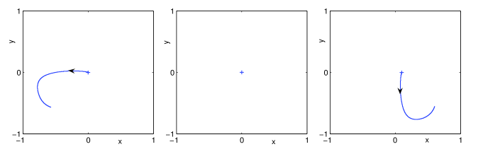
(b)

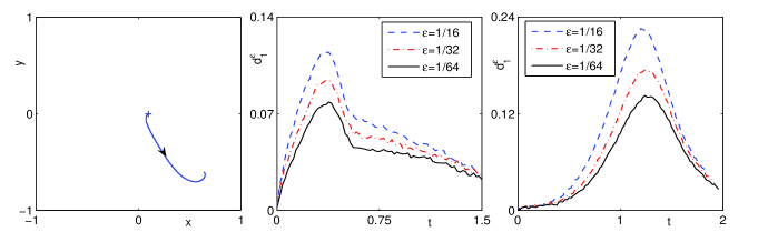
Figure 1: Trajectory of the vortex center in CGLE under Dirichlet BC when $\varepsilon=\frac{1}{32}$ under four cases, i.e. cases II-IV and VI, and the time evolution of $d_{1}^{\varepsilon}$ for different $\varepsilon$ under cases II and VI (from left to right and then from top to bottom) in section 4.1.

Fig. 1 shows the trajectory of the vortex center when $\varepsilon=\frac{1}{32}$ for cases II-IV and VI as well as the time evolution of $d_{1}^{\varepsilon}(t)$ for different $\varepsilon$ for cases II and VI, and the trajectory of the vortex center under cases V-VIII and cases IX-XII are, respectively, shown by Fig. 2 and Fig. 3 when $\varepsilon=\frac{1}{32}$ in CGLE. Based on these ample numerical results (although some results are not shown here for brevity), we made the following observations for the single vortex dynamics:

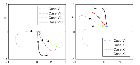
Figure 2: Trajectory of the vortex center in CGLE under Dirichlet BC when $\varepsilon=\frac{1}{32}$ under cases V-VIII (left) and cases IX-XII (right) in section 4.1.

(i). When $h({\bf x})\equiv 0$, the vortex center doesn’t move, which is similar to the vortex dynamics in the whole space in GLE and NLSE dynamics. (ii). When $h({\bf x})=(x+by)(x-\frac{y}{b})$ with $b\neq 0$, the vortex does not move if ${\bf x}_{0}=(0,0)$, while it does move if ${\bf x}_{0}\neq(0,0)$ (please see case III and VI for $b=1$). This is the same as the phenomena in GLE and NLSE dynamics. (iii). When $h({\bf x})\neq 0$ and $h({\bf x})\neq(x+by)(x-\frac{y}{b})$ with $b\neq 0$, in general, the vortex center does move to a different point from its initial location and then it will stay there forever. This is quite different from the corresponding case in the whole space, since in that case a single vortex may move to infinity under the initial data (4.1) with $h({\bf x})\neq 0$. (iv). In general, the initial location, the geometry of the domain and the boundary value will take effect on the motion of the vortex center. (v). When $\varepsilon\rightarrow 0$, the dynamics of the vortex center in the CGLE dynamics converges uniformly in time to that in the reduced dynamics (see Fig. 1) which verifies numerically the validation of the RDLs. In fact, based on our extensive numerical experiments, the motion of the vortex center from the RDLs agrees with those from the CGLE dynamics qualitatively when $0<\varepsilon<1$ and quantitatively when $0<\varepsilon\ll 1$.

(a)

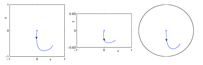
(b)

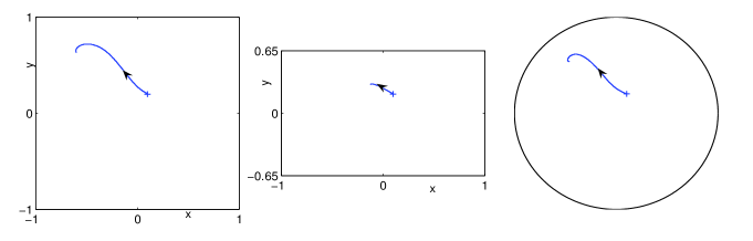
Figure 3: Trajectory of the vortex center in CGLE under Dirichlet BC when $\varepsilon=\frac{1}{32}$ for cases: (a) I, XIII, XIV, (b) X, XV, XVI (from left to right) in section 4.1.

4.2 Vortex pair

Here we present numerical results of the interaction of vortex pair in the CGLE dynamics and its corresponding reduced dynamics. In the following numerical simulations of the subsection, we take $M=2$, $n_{1}=n_{2}=1$, ${\bf x}_{1}^{0}=(-0.3,0)$ and ${\bf x}_{2}^{0}=(0.3,0)$ in (4.1). Fig. 4 depicts the trajectory of the vortex centers and their corresponding time evolution of the GL functionals when $\varepsilon=\frac{1}{25}$ in the CGLE with different $h({\bf x})$ in (4.1), and Fig. 5 shows contour plots of $|\psi^{\varepsilon}({\bf x},t)|$ for $\varepsilon=\frac{1}{25}$ at different times as well as the time evolution of ${\bf x}_{1}^{\varepsilon}(t)$, ${\bf x}_{1}^{\rm r}(t)$ and $d_{1}^{\varepsilon}(t)$ for different $\varepsilon$ with $h({\bf x})=0$ in (4.1).

(a)

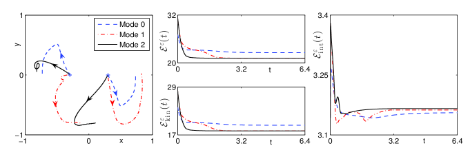
(b)

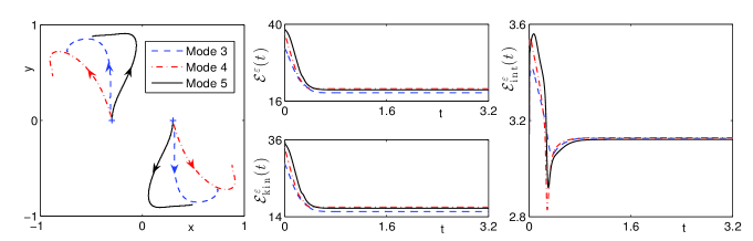
Figure 4: Trajectory of the vortex centers (a) and their corresponding time evolution of the GL functionals (b) in CGLE dynamics under Dirichlet BC when $\varepsilon=\frac{1}{25}$ with different $h({\bf x})$ in (4.1) in section 4.2.

According to our ample numerical experiments, we made the following observations for the interaction of vortex pair in the CGLE dynamics with Dirichlet BC: (i). The motion of the vortex pair may be thought of as a kind of combination between that in the GLE and NLSE dynamics with Dirichlet BC. From Figs. 4-5, we observed that the two vortices undergo a repulsive interaction, and they first rotate with each other and meanwhile move apart from each other towards the boundary of the domain, then stop somewhere near the boundary, which indicates that the boundary of the domain imposes a repulsive force on the two vortices. As shown in previous studies [7, 8], a vortex pair in the GLE dynamics moves outward along the line that connects with the two vortices and finally stay static near the boundary, while in the NLSE dynamics the two vortices always rotate around each other periodically. In fact, based on our extensive numerical results, we found that the larger the value $\beta$ (or $\alpha$) is, the closer the motion in CGLE dynamics is to that in NLSE (or GLE) dynamics, which gives the sufficient numerical evidence for our above conclusion. (ii). The phase shift $h({\bf x})$ affects the motion of the vortices significantly. When $h({\bf x})=(x+by)(x-\frac{y}{b})$ with $b\neq 0$, the vortices will move outward symmetric with respect to the origin, i.e., ${\bf x}_{1}(t)=-{\bf x}_{2}(t)$ (see Fig. 4). (iii). When $\varepsilon\rightarrow 0$, the dynamics of the two vortex centers in the CGLE dynamics converges uniformly in time to that in the reduced dynamics (see Fig. 5) which verifies numerically the validation of the RDLs in this case. In fact, based on our extensive numerical experiments, the motions of the two vortex centers from the RDLs agree with those from the CGLE dynamics qualitatively when $0<\varepsilon<1$ and quantitatively when $0<\varepsilon\ll 1$. (iv). During the dynamics evolution of CGLE, the GL functional and its kinetic part decrease as the time evolves, its interaction part changes dramatically when $t$ is small, and when $t\to\infty$, all the three quantities converge to constants (see Fig. 4), which immediately indicates that a steady state solution will be reached when $t\to\infty$.

 

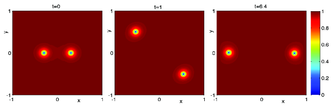
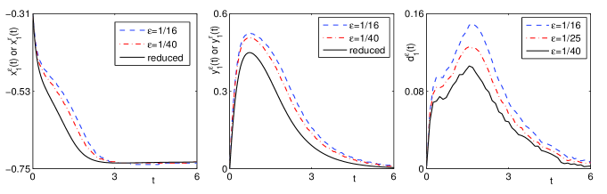
Figure 5: Contour plot of $|\psi^{\varepsilon}({\bf x},t)|$ for $\varepsilon=\frac{1}{25}$ at different times as well as time evolution of ${\bf x}_{1}^{\varepsilon}(t)$ in CGLE dynamics and ${\bf x}_{1}^{\rm r}(t)$ in the reduced dynamics under Dirichlet BC with $h({\bf x})=0$ in (4.1) and their difference $d_{1}^{\varepsilon}(t)$ for different $\varepsilon$ in section 4.2.

4.3 Vortex dipole

Here we present numerical results of the interaction of vortex dipole under the CGLE dynamics and its corresponding reduced dynamical laws. We choose the parameters in the simulations as $M=2$, $n_{1}=-n_{2}=-1$, ${\bf x}_{2}^{0}=-{\bf x}_{1}^{0}=(0.3,0)$ in (4.1). Fig. 6 depicts the trajectory of the vortex centers and their corresponding time evolution of the GL functionals when $\varepsilon=\frac{1}{25}$ in the CGLE with different $h({\bf x})$ in (4.1), and Fig. 7 shows contour plot of $|\psi^{\varepsilon}({\bf x},t)|$ for $\varepsilon=\frac{1}{25}$ at different times as well as the time evolution of ${\bf x}_{1}^{\varepsilon}(t)$, ${\bf x}_{1}^{\rm r}(t)$ and $d_{1}^{\varepsilon}(t)$ for different $\varepsilon$ with $h({\bf x})=0$ in (4.1).

(a)

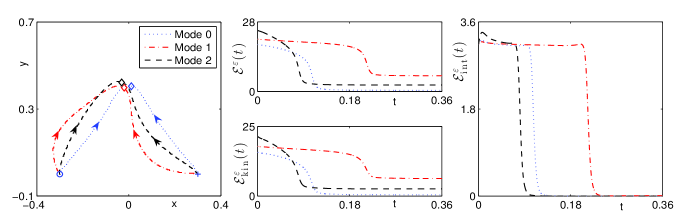
(b)

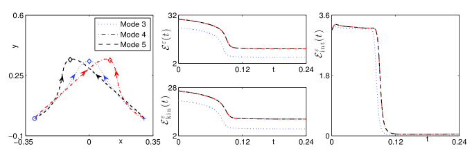
Figure 6: Trajectory of the vortex centers (a) and their corresponding time evolution of the GL functionals (b) in CGLE dynamics under Dirichlet BC when $\varepsilon=\frac{1}{25}$ with different $h({\bf x})$ in (4.1) in section 4.3.

From Figs. 6-7 and ample numerical experiments (not shown here for brevity), we made the following observations for the interaction of vortex dipole in the CGLE dynamics with Dirichlet BC: (i). The two vortices undergo an attractive interaction, they will collide and annihilate with each other. (ii). The phase shift $h({\bf x})$ and the initial distance of the two vortices affect the motion of the vortices significantly. If $h({\bf x})=0$, regardless of where the vortices are initially located, the vortex dipole will finally merge. However, similar as the case in GLE dynamics, if $h({\bf x})\not\equiv 0$, say $h({\bf x})=x+y$ for example, there would be a critical distance $d_{c}^{\varepsilon}$, which depends on the value of $\varepsilon$, that divides the motion of the vortex dipole into two cases: (a) if the initial distance between the vortex dipole $|{\bf x}_{2}^{0}-{\bf x}_{1}^{0}|>d_{c}^{\varepsilon}$, the vortex will never merge, they will finally stay static and separate at somewhere near the boundary. (b) otherwise, they do finally merge and annihilate. (iii). For $h({\bf x})=0$, when $\varepsilon\rightarrow 0$, the dynamics of the two vortex centers in the CGLE dynamics converges uniformly in time to that in the reduced dynamics (see Fig. 7), which verifies numerically the validation of the RDLs in this case. In fact, based on our extensive numerical experiments, the motions of the two vortex centers from the RDLs agree with those from the CGLE dynamics qualitatively when $0<\varepsilon<1$ and quantitatively when $0<\varepsilon\ll 1$ before they merge. (iv). During the dynamics evolution of CGLE, the GL functional decreases as the time evolves, its kinetic and interaction parts don’t change dramatically when $t$ is small, while all the three quantities converge to constants when $t\to\infty$. Moreover, if finite time merging/annihilation happens, the GL functional and its kinetic and interaction parts change significantly during the collision. In addition, when $t\to\infty$, the interaction energy goes to $0$ which immediately implies that a steady state will be reached in the form of $\phi^{\varepsilon}({\bf x})=e^{ic({\bf x})}$, where $c({\bf x})$ is a harmonic function satisfying $c({\bf x})|_{\partial\mathcal{D}}=h({\bf x})+\sum_{j=1}^{M}n_{j}\theta({\bf x}-{\bf x}^{0}_{j})$.

 

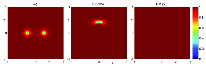
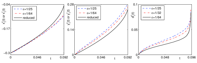
Figure 7: Contour plots of $|\psi^{\varepsilon}({\bf x},t)|$ for $\varepsilon=\frac{1}{25}$ at different times as well as time evolution of ${\bf x}_{1}^{\varepsilon}(t)$ in CGLE dynamics, ${\bf x}_{1}^{\rm r}(t)$ in the reduced dynamics under Dirichlet BC with $h({\bf x})=0$ in (4.1) and their difference $d_{1}^{\varepsilon}(t)$ for different $\varepsilon$ in section 4.3.

4.4 Vortex lattice

Here we present numerical results about the interaction of vortex lattices under the CGLE dynamics. We consider the following 15 cases: case I. $M=3$, $n_{1}=n_{2}=n_{3}=1$, ${\bf x}_{1}^{0}=(0.5,0)$; ${\bf x}_{2}^{0}=(-0.25,\frac{\sqrt{3}}{4})$, ${\bf x}_{3}^{0}=(-0.25,-\frac{\sqrt{3}}{4})$, case II. $M=3$, $n_{1}=n_{2}=n_{3}=1$, ${\bf x}_{1}^{0}=(-0.4,0)$, ${\bf x}_{2}^{0}=(0,0)$, ${\bf x}_{3}^{0}=(0.4,0)$; case III. $M=3$, $n_{1}=n_{2}=n_{3}=1$, ${\bf x}_{1}^{0}=(0,0.3)$, ${\bf x}_{2}^{0}=(0.15,0.15)$, ${\bf x}_{3}^{0}=(0.3,0)$; case IV. $M=3$, $-n_{1}=n_{2}=n_{3}=1$, ${\bf x}_{1}^{0}=(0.5,0)$; ${\bf x}_{2}^{0}=(-0.25,\frac{\sqrt{3}}{4})$, ${\bf x}_{3}^{0}=(-0.25,-\frac{\sqrt{3}}{4})$, case V. $M=3$, $n_{2}=-1$, $n_{1}=n_{3}=1$, ${\bf x}_{1}^{0}=(-0.4,0)$, ${\bf x}_{2}^{0}=(0,0)$, ${\bf x}_{3}^{0}=(0.4,0)$; case VI. $M=3$, $n_{1}=-1$, $n_{2}=n_{3}=1$, ${\bf x}_{1}^{0}=(0.2,0.3)$, ${\bf x}_{2}^{0}=(-0.3,0.4)$, ${\bf x}_{3}^{0}=(-0.4,-0.2)$; case VII. $M=4$, $n_{1}=n_{2}=n_{3}=n_{4}=1$, ${\bf x}_{1}^{0}=(0.5,0)$, ${\bf x}_{2}^{0}=(0,0.5)$, ${\bf x}_{3}^{0}=(-0.5,0)$, ${\bf x}_{4}^{0}=(0,-0.5)$; case VIII. $M=4$, $n_{1}=n_{3}=1$, $n_{2}=n_{4}=-1$, ${\bf x}_{1}^{0}=(0.5,0)$, ${\bf x}_{2}^{0}=(0,0.5)$, ${\bf x}_{3}^{0}=(-0.5,0)$, ${\bf x}_{4}^{0}=(0,-0.5)$; case IX. $M=4$, $n_{2}=n_{3}=-1$, $n_{1}=n_{4}=1$, ${\bf x}_{1}^{0}=(0.5,0)$, ${\bf x}_{2}^{0}=(0,0.5)$, ${\bf x}_{3}^{0}=(-0.5,0)$, ${\bf x}_{4}^{0}=(0,-0.5)$; case X. $M=4$, $n_{1}=n_{3}=1$, $n_{2}=n_{4}=-1$, ${\bf x}_{1}^{0}=(0.5,0.5)$, ${\bf x}_{2}^{0}=(-0.5,0.5)$, ${\bf x}_{3}^{0}=(-0.5,-0.5)$, ${\bf x}_{4}^{0}=(0.5,-0.5)$; case XI. $M=4$, $n_{2}=n_{3}=-1$, $n_{1}=n_{4}=1$, ${\bf x}_{1}^{0}=(0.5,0.5)$, ${\bf x}_{2}^{0}=(-0.5,0.5)$, ${\bf x}_{3}^{0}=(-0.5,-0.5)$, ${\bf x}_{4}^{0}=(0.5,-0.5)$; case XII. $M=4$, $n_{1}=n_{3}=-1$, $n_{2}=n_{4}=1$, ${\bf x}_{1}^{0}=(0.4,0)$, ${\bf x}_{2}^{0}=(-0.4/3,0)$, ${\bf x}_{3}^{0}=(0.4/3,0)$, ${\bf x}_{4}^{0}=(0.4,0)$; case XIII. $M=4$, $n_{2}=n_{3}=-1$, $n_{1}=n_{4}=1$, ${\bf x}_{1}^{0}=(0.4,0)$, ${\bf x}_{2}^{0}=(-0.4/3,0)$, ${\bf x}_{3}^{0}=(0.4/3,0)$, ${\bf x}_{4}^{0}=(0.4,0)$; case XIV. $M=4$, $n_{1}=n_{2}=-1$, $n_{3}=n_{4}=1$, ${\bf x}_{1}^{0}=(0.4,0)$, ${\bf x}_{2}^{0}=(-0.4/3,0)$, ${\bf x}_{3}^{0}=(0.4/3,0)$, ${\bf x}_{4}^{0}=(0.4,0)$; case XV. $M=4$, $n_{1}=n_{3}=-1$, $n_{2}=n_{4}=1$, ${\bf x}_{1}^{0}=(0.2,0.3)$, ${\bf x}_{2}^{0}=(-0.3,0.4)$, ${\bf x}_{3}^{0}=(-0.4,-0.2)$; ${\bf x}_{4}^{0}=(0.3,-0.3)$.

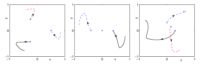
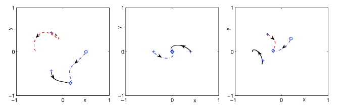
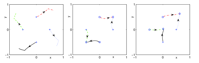
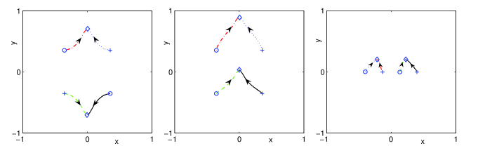
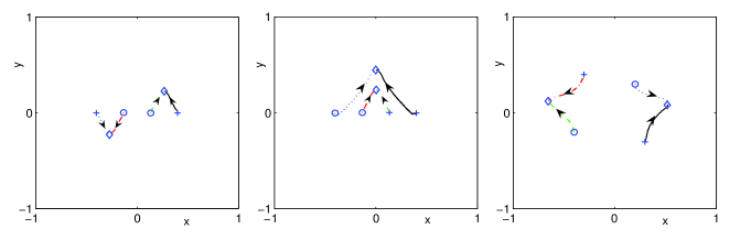
Figure 8: Trajectory of vortex centers for the interaction of different vortex lattices in GLE under Dirichlet BC with $\varepsilon=\frac{1}{32}$ and $h({\bf x})=0$ for cases I-IX (from left to right and then from top to bottom) in section 4.4.

Fig. 8 shows the trajectory of the vortex centers when $\varepsilon=\frac{1}{32}$ in CGLE (1.1) and $h({\bf x})=0$ in (4.1) for the above 15 cases. From Fig. 8 and ample numerical experiments (not shown here for brevity), we made the following observations: (i). The dynamics and interaction of vortex lattices under the CGLE dynamics with Dirichlet BC depends on its initial alignment of the lattice, geometry of the domain $\mathcal{D}$ and the boundary value $g({\bf x})$. (ii). For a lattice of $M$ vortices, if they have the same index, then no collisions will happen for any time $t\geq 0$. On the other hand, if they have opposite index, e.g. $M^{+}>0$ vortices with index ‘$+1$’ and $M^{-}>0$ vortices with index ‘$-1$’ satisfying $M^{+}+M^{-}=M$, collisions will always happen at finite time. More precisely, when $t$ is sufficiently large, there exist exactly $|M^{+}-M^{-}|$ vortices with winding number ‘$+1$’ if $M^{+}>M^{-}$; while if $M^{+}<M^{-}$, there exist exactly $|M^{+}-M^{-}|$ vortices with winding number ‘$-1$’.

(a) 

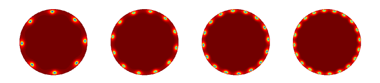
(b) 

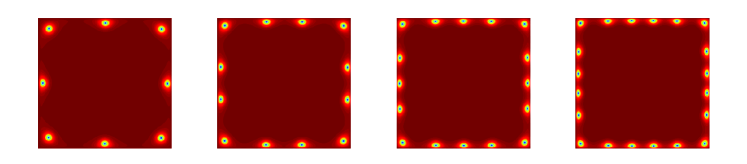
(c) 

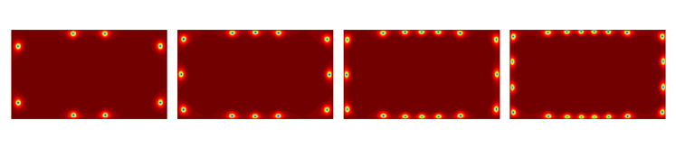
Figure 9: Contour plots of $|\phi^{\varepsilon}({\bf x})|$ for the steady states of vortex lattice in CGLE under Dirichlet BC with $\varepsilon=\frac{1}{32}$ for $M=8,\;12,\;16,\;20$ (from left column to right column) and different domains: (a) unit disk $\mathcal{D}=B_{1}({\bf 0})$, (b) square domain $\mathcal{D}=[-1,1]^{2}$, (c) rectangular domain $\mathcal{D}=[-1.6,1.6]\times[-0.8,0.8]$.

In order to study how the geometry of the domain and boundary conditions take effect on the alignment of vortices in the steady state patterns in the CGLE dynamics under Dirichlet BC, we made the following set-up for our numerical computations. We chose the parameters as $\varepsilon=\frac{1}{32}$,

$$n_{j}=1,\qquad{\bf x}_{j}^{0}=0.5\left(\cos\left(\frac{2j\pi}{M}\right),\sin\left(\frac{2j\pi}{M}\right)\right),\qquad j=1,2,\ldots,M,$$

i.e., initially we have $M$ like vortices which are located uniformly in a circle centered at origin with radius $R_{1}=0.5$. Denote $\phi^{\varepsilon}({\bf x})$ as the steady state, i.e., $\phi^{\varepsilon}({\bf x})=\lim_{t\to\infty}\psi^{\varepsilon}({\bf x},t)$ for ${\bf x}\in\mathcal{D}$. Fig. 9 depicts the contour plots of the amplitude $|\phi^{\varepsilon}|$ of the steady state in the CGLE dynamics with $h({\bf x})=0$ in (4.1) for different $M$ and domains, and Fig. 10 depicts similar results with $M=12$ for different $h({\bf x})$ in (4.1).

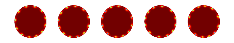
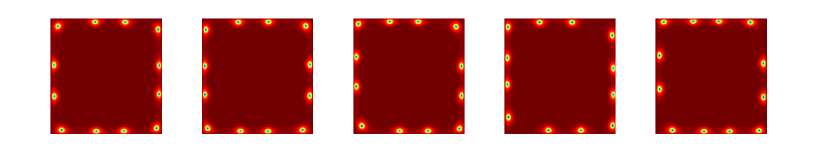
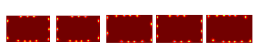
Figure 10: Contour plots of $|\phi^{\varepsilon}({\bf x})|$ for the steady states of vortex lattice in CGLE under Dirichlet BC with $\varepsilon=\frac{1}{32}$ and $M=12$ on a unit disk $\mathcal{D}=B_{1}({\bf 0})$ (top row) or a square $\mathcal{D}=[-1,1]^{2}$ (middle row) or a rectangular domain $\mathcal{D}=[-1.6,1.6]\times[-0.8,0.8]$ (bottom row) under different $h({\bf x})=x+y,\;x^{2}-y^{2},\ x-y,\;x^{2}-y^{2}+2xy,\;x^{2}-y^{2}-2xy$ (from left column to right column).

Based on Figs. 9-10 and ample numerical results (not shown here for brevity), we made the following observations for the steady state patterns of vortex lattices under the CGLE dynamics with Dirichlet BC: (i). The vortex lattices with the same winding number undergo repulsive interaction between each other and finally they move to somewhere near the boundary of the domain. During the evolution process, no particle-like collision phenomena happen and a steady state pattern is finally formed when $t\to\infty$. As a matter of fact, the steady state is also the solution of the following minimization problem

$$\phi^{\varepsilon}=\displaystyle{\rm argmin}_{\phi({\bf x})|_{{\bf x}\in\partial\mathcal{D}}=\psi_{0}^{\varepsilon}({\bf x})|_{{\bf x}\in\partial\mathcal{D}}}\mathcal{E}^{\varepsilon}(\phi).$$

(ii). Both the geometry of the domain and the phase shift, i.e. $h({\bf x})$, will take significant effect on steady state patterns. (iii). At the steady state, the distance between the vortex centers and the boundary of the domain depends on $\varepsilon$ and $M$. If $M$ is fixed, when $\varepsilon$ decreases, the distance decreases; while if $\varepsilon$ is fixed, when $M$ increases, the distance decreases. We remark it here as an interesting open problem to find how the width depends on the value of $\varepsilon$, the boundary condition as well as the geometry of the domain.

5 Numerical results under Neumann BC

In this section, we report numerical results for vortex interactions of the CGLE (1.1) under the homogeneous Neumann BC (1.4) and compare them with those obtained from the corresponding RDLs. The initial condition $\psi_{0}^{\varepsilon}$ in (1.2) is also chosen as the form (4.1), but with harmonic function $h({\bf x})$ replaced as $h_{n}({\bf x})$ so that it will satisfy the Neumann BC as

$$\frac{\partial}{\partial{\bf n}}h_{n}({\bf x})=-\frac{\partial}{\partial{\bf n}}\sum_{l=1}^{M}n_{l}\theta({\bf x}-{\bf x}_{l}^{0}),\quad{\bf x}\in\partial\Omega.$$

The CGLE (1.1) with (1.4) and (4.1) is solved by the numerical method TSCP presented in section 3 in the following simulations.

5.1 Single vortex

In the subsection, we present numerical results of the motion of a single quantized vortex in the CGLE dynamics with Neumann BC and its corresponding reduced dynamical laws. We choose the parameters as $M=1$ and $n_{1}=1$ in (4.1). Fig. 11 shows the trajectory of the vortex center for different ${\bf x}_{1}^{0}$ in (4.1) when $\varepsilon=\frac{1}{25}$ as well as time evolution of ${\bf x}_{1}^{\varepsilon}$ and $d_{1}^{\varepsilon}$ for different $\varepsilon$.

By observing Fig. 11 and ample numerical simulation results (not shown here for brevity), we could see that: (i). The initial location of the vortex affects the motion of the vortex significantly and this reflects the boundary effect coming from the Neumann BC. (ii). If ${\bf x}_{1}^{0}=(0,0)$, the vortex does not move at any time; otherwise, the vortex does move and it will run out of the domain and never come back. This phenomenon is quite different from the case with Dirichlet BC in bounded domains, in which a single vortex can never move out of the domain, or the case with the initial condition (4.1) in the whole space, in which a single vortex doesn’t move at all, regardless of the initial location of the vortex for the both cases. (iii). As $\varepsilon\rightarrow 0$, the dynamics of the vortex center under the CGLE dynamics converges uniformly in time to that of the RDLs very well before it exits the domain, which verifies numerically the validation of the RDLs in this case. Apparently, when the vortex center moves out of the domain, the reduced dynamics laws are no longer valid. Based on our extensive numerical experiments, the motion of the vortex center from the RDLs agrees with that from the CGLE dynamics qualitatively when $0<\varepsilon<1$ and quantitatively when $0<\varepsilon\ll 1$ before it moves out of the domain.

(a)

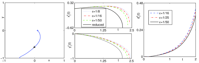
(b)

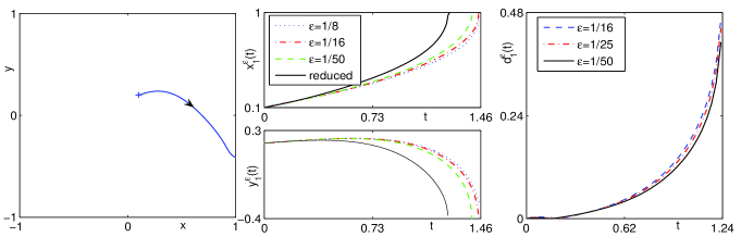
Figure 11: Trajectory of the vortex center when $\varepsilon=\frac{1}{25}$ (left) as well as time evolution of ${\bf x}_{1}^{\varepsilon}$ (middle) and $d_{1}^{\varepsilon}$ for different $\varepsilon$ (right) for the motion of a single vortex in CGLE under homogeneous Neumann BC with different ${\bf x}_{1}^{0}$ in (4.1) in section 5.1: (a) ${\bf x}_{1}^{0}=(0.1,0)$, (b) ${\bf x}_{1}^{0}=(0.1,0.2)$.

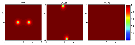
(a) (c)

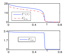
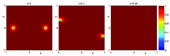
(b) (d)

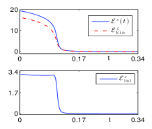
Figure 12: Contour plots of $|\psi^{\varepsilon}({\bf x},t)|$ at different times when $\varepsilon=\frac{1}{25}$ ((a) & (b)) and the corresponding time evolution of the GL functionals ((c) & (d)) for the motion of vortex pair in CGLE under homogeneous Neumann BC with different $d_{0}$ in (4.1) in section 5.2: top row: $d_{0}=0.3$, bottom row: $d_{0}=0.7$.

5.2 Vortex pair

Here we present numerical results of the interaction of vortex pair under the CGLE dynamics with Neumann BC and its corresponding reduced dynamical laws. We choose the simulation parameters as $M=2$, $n_{1}=n_{2}=1$ and ${\bf x}_{2}^{0}=-{\bf x}_{1}^{0}=(d_{0},0)$ with $0<d_{0}<1$ in (4.1). Fig. 12 shows the contour plots of $|\psi^{\varepsilon}({\bf x},t)|$ at different times when $\varepsilon=\frac{1}{25}$, and Fig. 13 shows the trajectory of the vortex pair when $\varepsilon=\frac{1}{25}$ as well as time evolution of $x_{1}^{\varepsilon}(t)$ and $d_{1}^{\varepsilon}(t)$ for different $d_{0}$ in (4.1).

(a)

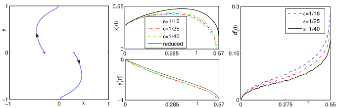
(b)

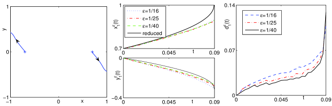
Figure 13: Trajectory of the vortex center when $\varepsilon=\frac{1}{25}$ (left) as well as time evolution of ${\bf x}_{1}^{\varepsilon}$ (middle) and $d_{1}^{\varepsilon}$ for different $\varepsilon$ (right) for the motion of vortex pair in CGLE under homogeneous Neumann BC with different $d_{0}$ in (4.1) in section 5.2: (a) $d_{0}=0.3$, (b) $d_{0}=0.7$.

From Figs. 12-13 and ample numerical results (not shown here for brevity), we made the following observations: (i). The initial location of the vortex, i.e., the value of $d_{0}$ affects the motion of the vortex significantly and this reflects the boundary effect coming from the Neumann BC. (ii). For the CGLE with $\varepsilon$ fixed, there exists a sequence of critical values $d_{1}^{c,\varepsilon}>d_{2}^{c,\varepsilon}>d_{3}^{c,\varepsilon}>\cdots>d_{k}^{c,\varepsilon}>\cdots$, which can determine the escape approach about how the vortex pair moves out of the domain. More precisely, if the value of $d_{0}$ falls into the interval $(d_{2n+1}^{c,\varepsilon},d_{2n}^{c,\varepsilon})$, where $n=0,1,\ldots$, and $d_{0}^{c,\varepsilon}=+\infty$, then the two vortices will move out of the domain from the side boundary; otherwise, if it falls into the interval $(d_{2n+2}^{c,\varepsilon},d_{2n+1}^{c,\varepsilon})$, they will move out of the domain from the top-bottom boundary. For the RDL, there also exists such corresponding sequence of critical values $\{d_{k}^{c,r},k=0,1,\ldots\}$ which determine the trajectory of the vortex pair motion. We note that it might be an interesting problem to find the values of those $d_{k}^{c,\varepsilon}$ and $d_{k}^{c,r}$ and study their convergence relations between them. (iii). The motion of the vortex pair exhibits hybrid properties of that in the GLE dynamics and NLSE dynamics with Neumann BC. As given by previous studies [7, 8], a vortex pair in the GLE dynamics will always move outward along the line that connects with the two vortices and finally they will move out of the domain, while in the NLSE dynamics, they will always rotate around each other periodically. Based on our extensive numerical results, we also found that under a fixed initial setup, the larger the value $\beta$ becomes, the more rotations the vortex pair will do before they exit the domain, which means that as $\beta$ becomes larger, the closer the motion in CGLE dynamics is to that in NLSE dynamics; on the other hand, as the value $\alpha$ becomes larger, the time when the vortex pair exits the domain becomes faster, which also means that the motion in CGLE dynamics becomes closer to that in GLE dynamics. This gives sufficient numerical evidence for our conclusion. (iv). As $\varepsilon\rightarrow 0$, the dynamics of the vortex pair under the CGLE dynamics converges uniformly in time to that of the RDLs very well before either of the two vortices exit the domain, which verifies numerically the validation of the RDLs in this case. (iv). During the dynamics evolution of CGLE, the GL functional and its kinetic parts decrease as the time increases. They do not change much when $t$ is small and change dramatically when either of the two vortices move out of the domain. When $t\to\infty$, all the three quantities converge to 0 (see Fig. 12 (c) & (d)), which indicates that a constant steady state have been reached in the form of $\phi^{\varepsilon}({\bf x})=e^{ic_{{}_{0}}}$ for ${\bf x}\in\mathcal{D}$ with $c_{{}_{0}}$ a constant.

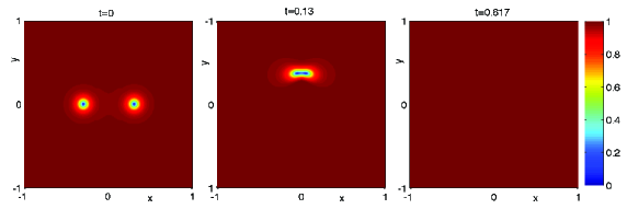
(a) (c)

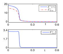
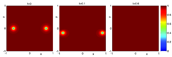
(b) (d)

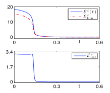
Figure 14: Contour plots of $|\psi^{\varepsilon}({\bf x},t)|$ at different times when $\varepsilon=\frac{1}{25}$ and the corresponding time evolution of the GL functionals for the motion of vortex dipole in CGLE under homogeneous Neumann BC with different $d_{0}$ in (4.1) in section 5.3: top row: $d_{0}=0.3$, bottom row: $d_{0}=0.7$.

5.3 Vortex dipole

Here we present numerical results of the interaction of vortex dipole in the CGLE dynamics with Neumann BC and its corresponding reduced dynamics. We choose the simulation parameters as $M=2$, $n_{2}=-n_{1}=1$ and ${\bf x}_{2}^{0}=-{\bf x}_{1}^{0}=(d_{0},0)$ with $0<d_{0}<1$ in (4.1). Fig. 14 shows the contour plots of $|\psi^{\varepsilon}({\bf x},t)|$ at different times when $\varepsilon=\frac{1}{25}$, and Fig. 15 depicts the trajectory of the vortex pair when $\varepsilon=\frac{1}{25}$ as well as time evolution of $x_{1}^{\varepsilon}(t)$ and $d_{1}^{\varepsilon}(t)$ for different $d_{0}$ in (4.1).

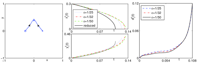
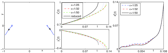
Figure 15: Trajectory of the vortex center when $\varepsilon=\frac{1}{25}$ (left) as well as time evolution of ${\bf x}_{1}^{\varepsilon}$ (middle) and $d_{1}^{\varepsilon}$ for different $\varepsilon$ (right) for the motion of vortex dipole in CGLE under homogeneous Neumann BC with different $d_{0}$ in (4.1) in section 5.2: (a) $d_{0}=0.3$, (b) $d_{0}=0.7$.

From Fig. 14 and 15 and ample numerical results (not shown here for brevity), we can make the following observations for the interaction of vortex pair under the NLSE dynamics with homogeneous Neumann BC: (i). The initial location of the vortex, i.e., the value of $d_{0}$ affects the motion of the vortex significantly. (ii). For the CGLE with $\varepsilon$ fixed, there exists a critical value $d_{c}^{\varepsilon}$ such that: if $d_{0}>d_{c}^{\varepsilon}$, the two vortices will exit the domain from the side boundary; otherwise, they will merge somewhere in the domain. For the RDL, there also exists such corresponding critical values $d_{c}^{r}$. We also note that it might be an interesting problem to find those values $d_{c}^{\varepsilon}$ and $d_{c}^{r}$, and to study their convergence relation. (iii). As $\varepsilon\rightarrow 0$, the dynamics of the two vortex centers under the CGLE dynamics converge uniformly in time to that of the RDLs very well before they move out of the domain or merge with each other, which verifies numerically the validation of the RDLs in this case.

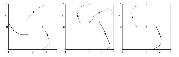
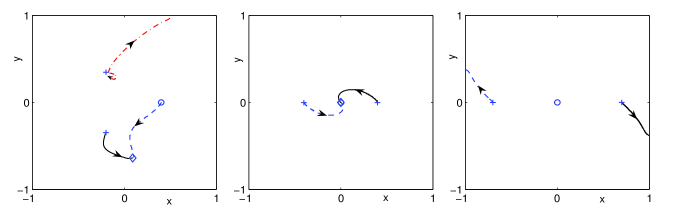
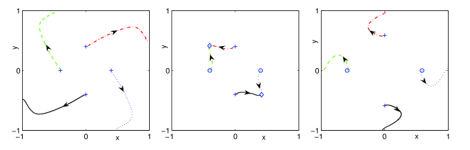
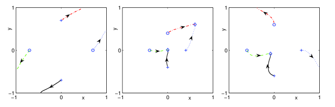
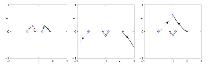
Figure 16: Trajectory of vortex centers for the interaction of different vortex lattices in CGLE under Neumman BC with $\varepsilon=\frac{1}{32}$ for cases I-IX (from left to right and then from top to bottom) in section 5.4.

5.4 Vortex lattice

Here we present numerical results of the interaction of vortex lattices under the CGLE dynamics with Neumann BC. We consider the following 15 cases:

case I. $M=3$, $n_{1}=n_{2}=n_{3}=1$, ${\bf x}_{1}^{0}=(0.4,0)$, ${\bf x}_{2}^{0}=(-0.2,\frac{\sqrt{3}}{5})$, ${\bf x}_{3}^{0}=(-0.2,-\frac{\sqrt{3}}{5})$; case II. $M=3$, $n_{1}=n_{2}=n_{3}=1$, ${\bf x}_{1}^{0}=(-0.4,0.2)$, ${\bf x}_{2}^{0}=(0,0.2)$, ${\bf x}_{3}^{0}=(0.4,0.2)$; case III. $M=3$, $n_{1}=n_{2}=n_{3}=1$, ${\bf x}_{1}^{0}=(-0.4,0)$, ${\bf x}_{2}^{0}=(0,0)$, ${\bf x}_{3}^{0}=(0.4,0)$; case IV. $M=3$, $-n_{1}=n_{2}=n_{3}=1$, ${\bf x}_{1}^{0}=(0.4,0)$; ${\bf x}_{2}^{0}=(-0.2,\frac{\sqrt{3}}{5})$, ${\bf x}_{3}^{0}=(-0.2,-\frac{\sqrt{3}}{5})$; case V. $M=3$, $-n_{2}=n_{1}=n_{3}=1$, ${\bf x}_{1}^{0}=(-0.4,0)$, ${\bf x}_{2}^{0}=(0,0)$, ${\bf x}_{3}^{0}=(0.4,0)$; case VI. $M=3$, $-n_{2}=n_{1}=n_{3}=1$, ${\bf x}_{1}^{0}=(-0.7,0)$, ${\bf x}_{2}^{0}=(0,0)$, ${\bf x}_{3}^{0}=(0.7,0)$; case VII. $M=4$, $n_{1}=n_{2}=n_{3}=n_{4}=1$, ${\bf x}_{1}^{0}=(0.4,0)$, ${\bf x}_{2}^{0}=(0,0.4)$, ${\bf x}_{3}^{0}=(-0.4,0)$, ${\bf x}_{4}^{0}=(0,-0.4)$; case VIII. $M=4$, $n_{1}=n_{3}=-1$, $n_{2}=n_{4}=1$, ${\bf x}_{1}^{0}=(0.4,0)$, ${\bf x}_{2}^{0}=(0,0.4)$, ${\bf x}_{3}^{0}=(-0.4,0)$, ${\bf x}_{4}^{0}=(0,-0.4)$; case IX. $M=4$, $n_{1}=n_{3}=-1$, $n_{2}=n_{4}=1$, ${\bf x}_{1}^{0}=(0.59,0)$, ${\bf x}_{2}^{0}=(0,0.59)$, ${\bf x}_{3}^{0}=(-0.59,0)$, ${\bf x}_{4}^{0}=(0,-0.59)$; case X. $M=4$, $n_{1}=n_{3}=-1$, $n_{2}=n_{4}=1$, ${\bf x}_{1}^{0}=(0.7,0)$, ${\bf x}_{2}^{0}=(0,0.7)$, ${\bf x}_{3}^{0}=(-0.7,0)$, ${\bf x}_{4}^{0}=(0,-0.7)$; case XI. $M=4$, $n_{2}=n_{3}=-1$, $n_{1}=n_{4}=1$, ${\bf x}_{1}^{0}=(0.4,0)$, ${\bf x}_{2}^{0}=(0,0.4)$, ${\bf x}_{3}^{0}=(-0.4,0)$, ${\bf x}_{4}^{0}=(0,-0.4)$; case XII. $M=4$, $n_{2}=n_{3}=-1$, $n_{1}=n_{4}=1$, ${\bf x}_{1}^{0}=(0.6,0)$, ${\bf x}_{2}^{0}=(0,0.6)$, ${\bf x}_{3}^{0}=(-0.6,0)$, ${\bf x}_{4}^{0}=(0,-0.6)$; case XIII. $M=4$, $n_{1}=n_{3}=-1$, $n_{2}=n_{4}=1$, ${\bf x}_{1}^{0}=(0.4,0)$, ${\bf x}_{2}^{0}=(-0.4/3,0)$, ${\bf x}_{3}^{0}=(0.4/3,0)$, ${\bf x}_{4}^{0}=(0.4,0)$; case XIV. $M=4$, $n_{1}=n_{3}=-1$, $n_{2}=n_{4}=1$, ${\bf x}_{1}^{0}=(0.4,0)$, ${\bf x}_{2}^{0}=(-0.4/3,0)$, ${\bf x}_{3}^{0}=(0.4/3,0)$, ${\bf x}_{4}^{0}=(0.4,0)$; case XV. $M=4$, $n_{1}=n_{3}=-1$, $n_{2}=n_{4}=1$, ${\bf x}_{1}^{0}=(-0.6,0)$, ${\bf x}_{2}^{0}=(-0.1,0)$, ${\bf x}_{3}^{0}=(0.1,0)$, ${\bf x}_{4}^{0}=(0.6,0)$.

Fig. 16 shows the trajectory of the vortex centers for the above 15 cases when $\varepsilon=\frac{1}{32}$, and Fig. 17 depicts the contour plots of $|\psi^{\varepsilon}|$ for the initial data and corresponding steady states for cases I, III, V, VI, VII and XIV. From Figs. 16 and 17 and ample numerical experiments (not shown here for brevity), we can make the following observations: (i). The dynamics and interaction of vortex lattices under the CGLE dynamics with Dirichlet BC depends on its initial alignment of the lattice, geometry of the domain $\mathcal{D}$. (ii). For a lattice of $M$ vortices, if they have the same index, then at least $M-1$ vortices will move out of the domain at finite time and no collision will happen at any time; On the other hand, if they have opposite index, collision will happen at finite time. After collisions, the leftover vortices will continue to move and at most one vortex may be left in the domain. When $t$ is sufficiently large, in most cases, no vortex can be left in the domain; but when the geometry and initial setup are properly set to be symmetric and $M$ is odd, there maybe one vortex left in the domain. (iii). If finally no vortex can be left in the domain, the GL functionals will always vanish as $t\rightarrow\infty$, which indicates that the final steady state always admits the form of $\phi^{\varepsilon}({\bf x})=e^{ic_{0}}$ for ${\bf x}\in\mathcal{D}$ with $c_{0}$ a real constant.

(a)

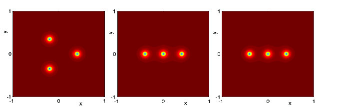
(b)

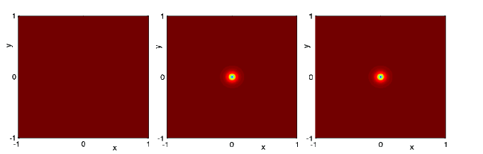
(c)

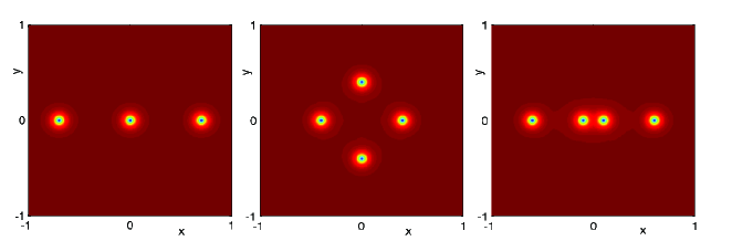
(d)

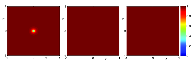
Figure 17: Contour plots of $|\psi^{\varepsilon}({\bf x},t)|$ for the initial data ((a) & (c)) and corresponding steady states ((b) & (d)) of vortex lattice in CGLE dynamics under Neumman BC with $\varepsilon=\frac{1}{32}$ and for cases I, III, V, VI, VII and XIV (from left to right and then from top to bottom) in section 5.4.

6 Conclusion

In this paper, we proposed efficient and accurate numerical methods to simulate complex Ginzburg-Landau equation (CGLE) with a dimensionless parameter $0<\varepsilon<1$ on bounded domains with either Dirichlet or homogenous Neumann BC and its corresponding reduced dynamical laws (RDLs). By these numerical methods, we studied numerically vortex dynamics and interaction in the CGLE and compared them with those obtained from the corresponding RDLs under different initial setups. To some extent, we found that vortex dynamics in the CGLE is a hybrid of that in GLE and NLSE, which can be reflected from the fact that CGLE is a combination equation between GLE and NLSE.

Based on our extensive numerical results, we verified that the dynamics of vortex centers under the CGLE dynamics converges to that of the RDLs when $\varepsilon\to 0$ before they collide and/or move out of the domain. Apparently, when the vortex center moves out of the domain, the reduced dynamics laws are no longer valid; however, the dynamics and interaction of quantized vortices are still physically interesting and they can be obtained from the direct numerical simulations for the CGLE with fixed $\varepsilon>0$ even after they collide and/or move out of the domain. We also identified the parameter regimes where the RDLs agree with qualitatively and/or quantitatively as well as fail to agree with those from the CGLE dynamics. Some very interesting nonlinear phenomena related to the quantized vortex interactions in the CGLE were also observed from our direct numerical simulation results of CGLE. Different steady state patterns of vortex lattices under the CGLE dynamics were obtained numerically. From our numerical results, we observed that both boundary conditions and domain geometry affect significantly on vortex dynamics and interaction, which can exhibit different interaction patterns compared with those in the whole space case [49, 50].

References

- [1] A. Aftalion and Q. Du, Vortices in a rotating Bose–Einstein condensate: critical angular velocities and energy diagrams in the Thomas–Fermi regime, Phys. Rev. A, 64 (2001), article 063603.
- [2] B. P. Anderson, Experiment with vortices in superfluid atomic gases, J. Low Temp. Phys., 161 (2010), 574–602.
- [3] I. S. Aranson and L. Kramer, The world of the complex Ginzburg–Landau equation, Rev. Mod. Phys., 74 (2002), 99–133.
- [4] W. Bao, Numerical methods for the nonlinear Schrödinger equation with nonzero far–field conditions, Methods Appl. Anal., 11 (2004), 367–388.
- [5] W. Bao, Q. Du and Y. Zhang, Dynamics of rotating Bose-Einstein condensates and their efficient and accurate numerical computation, SIAM J. Appl. Math., 66 (2006), 758–786.
- [6] W. Bao, S. Jin and P. A. Markowich, On time–splitting spectral approximations for the Schrödinger equation in the semiclassical regime, J. Comput. Phys., 175 (2002), 487–524.
- [7] W. Bao and Q. Tang, Numerical study of quantized vortex interaction in Ginzburg–Landau equation on bounded domains, Commun. Comput. Phys., 14 (2013), 819–850.
- [8] W. Bao and Q. Tang, Numerical study of quantized vortex interaction in nonlinear Schrödinger equation on bounded domains, preprint.
- [9] F. Bethuel, H. Brezis and F. Hélein, Ginzburg–Landau Vortices, Brikhäuser, 1994.
- [10] F. Bethuel, R. L. Jerrard and D. Smets, On the NLS dynamics for infinite energy vortex configurations on the plane, Rev. Mat. Iberoamericana, 24 (2008), 671–702.
- [11] F. Bethuel, G. Orlandi and D. Smets, Collisions and phase–vortex interactions in dissipative Ginzburg–Landau dynamics, Duke Math. J., 130 (2005), 523–614.
- [12] F. Bethuel, G. Orlandi and D. Smets, Dynamics of multiple degree Ginzburg–Landau vortices, Commun. Math. Phys., 272 (2007), 229–261.
- [13] F. Bethuel, G. Orlandi and D. Smets, Quantization and motion law for Ginzburg–Landau vortices, Arch. Rational Mech. Anal., 183 (2007), 315–370.
- [14] Z. Chen and S. Dai, Adaptive Galerkin methods with error control for a dynamical Ginzburg–Landau model in superconductivity, SIAM J. Numer. Anal., 38 (2001), 1961–1985.
- [15] J. E. Colliander and R. L. Jerrard, Ginzburg–Landau vortices: weak stability and Schrödinger equation dynamics, J. Anal. Math., 77 (1999), 129–205.
- [16] J. E. Colliander and R. L. Jerrard, Vortex dynamics for the Ginzburg–Landau–Schrödinger equation, IMRN Int. Math. Res. Not., 7 (1998), 333–358.
- [17] A. S. Desyatnikov, Y. S. Kivshar and L. Torner, Optical vortices and vortex solitons, Prog. Optics, 47 (2005), 291–391.
- [18] R. J. Donnelly, Quantized Vortices in Helium II, Cambridge University Press, 1991.
- [19] Q. Du, Finite element methods for the time dependent Ginzburg–Landau model of superconductivity, Comp. Math. Appl., 27 (1994), 119–133.
- [20] Q. Du, M. Gunzburger and J. Peterson, Analysis and approximation of the Ginzburg–Landau model of superconducting, SIAM Rev., 34 (1992), 54–81.
- [21] W. E, Dynamics of vortices in Ginzburg–Landau theroties with applications to superconductivity, Phys. D, 77 (1994), 38–404.
- [22] T. Frisch, Y. Pomeau and S. Rica, Transition to dissipation in a model of superflow, Phys. Rev. Lett., 69 (1992), 1644–1647.
- [23] V. Ginzburg and L. Pitaevskii, On the theory of superfluidity, Soviet Physics JETP, 34 (1958), 858–861.
- [24] R. Glowinski and P. Tallec, Augmented Lagrangian and Operator Splitting Method in Nonlinear Mechanics, SIAM, Philadelphia, PA, 1989.
- [25] R. L. Jerrard and H. Soner, Dynamics of Ginzburg–Landau vortices, Arch. Rational Mech. Anal., 142 (1998), 99–125.
- [26] R. L. Jerrard and D. Spirn, Refined Jacobian estimates and the Gross–Pitaevskii equations, Arch. Rational Mech. Anal., 190 (2008), 425–475.
- [27] S. Jimbo and Y. Morita, Notes on the limit equation of vortex equation of vortex motion for the Ginzburg–Landau equation with Neumann condition, Japan J. Indust. Appl. Math., 18 (1972), 151–200.
- [28] S. Jimbo and Y. Morita, Stability of nonconstant steady–state solutions to a Ginzburg–Landau equation in higer space dimension, Nonlinear Anal.: T.M.A., 22 (1994), 753–770.
- [29] S. Jimbo and Y. Morita, Vortex dynamics for the Ginzburg–Landau equation with Neumann condition, Methods App. Anal., 8 (2001), 451–477.
- [30] O. Karakashian and C. Makridakis, A space–time finite element method for the nonlinear Schrödinger equation: the discontinuous Galerkin method, Math. Comput., 67 (1998), 479–499.
- [31] M. Kurzke, C. Melcher, R. Moser and D. Spirn, Dynamics for Ginzburg–Landau vortices under a mixed flow, Indiana Univ. Math. J., 58 (2009), 2597–2622.
- [32] F. Lin, A remark on the previous paper “Some dynamical properties of Ginzburg–Landau vortices”, Comm. Pure Appl. Math., 49 (1996), 361–364.
- [33] F. Lin, Complex Ginzburg–Landau equations and dynamics of vortices, filaments, and codimension–2 submanifolds, Comm. Pure Appl. Math., 51 (1998), 385–441.
- [34] F. Lin, Some dynamical properties of Ginzburg-Landau vortices, Comm. Pure Appl. Math., 49 (1996), 323–359.
- [35] T. Lin, The stability of the radial solution to the Ginzburg–Landau equation, Comm. PDE., 22 (1997), 619–632.
- [36] F. Lin and J. Xin, A unified approach to vortex motion laws of complex scalar field equations, Math. Res. Lett., 5 (1998), 455–460.
- [37] F. Lin and J. Xin, On the incompressible fluid limit and the vortex motion law of the nonlinear Schrödinger equation, Comm. Math. Phys., 200 (1999), 249–274.
- [38] E. Miot, Dynamics of vortices for the complex Ginzburg–Landau equation, Anal. PDE, 2 (2009), 159–186.
- [39] P. Mironescu, On the stability of radial solutions of the Ginzburg–Landau equation, J. Funct. Anal., 130 (1995), 334–344.
- [40] J. Neu, Vortices in complex scalar fields, Phys. D, 43 (1990), 385-406.
- [41] C. Nore, M. E. Brachet, E. Cerda and E. Tirapegui, Scattering of first sound by superfluid vortices, Phys. Rev. Lett., 72 (1994), 2593–2595.
- [42] L. M. Pismen, Vortices in Nonlinear Fields, Clarendon, 1999.
- [43] P. H. Roberts and N. G. Berloff,“The nonlinear Schrödinger equation as a model of superfluidity,” in“Quantized Vortex Dynamics and Superfluid Turbulence”, C. F. Barenghi, R. J. Donnely, and W. F. Vinen, Springer, 2001.
- [44] E. Sandier and S. Serfaty, Gamma–convergence of gradient flows with applications to Ginzburg–Landau, Comm. Pure Appl. Math., 57 (2004), 1627–1672.
- [45] S. Serfaty, Vortex collisions and energy–dissipation rates in the Ginzburg–Landau heat flow. Part II: the dynamics, J. Euro. Math. Soc., 9 (2007), 383–426.
- [46] S. Serfaty, I. Tice, Ginzburg–Landau vortex dynamics with pinning and strong applied currents, Arch. Rational Mech. Anal., 201 (2011), 413-464.
- [47] J. Shen and T. Tang, Spectral and High–Order Method with Applications, Science Press, 2006.
- [48] G. Strang, On the construction and comparision of difference schemes, SIAM J. Numer. Anal., 5 (1968), 505–517.
- [49] Y. Zhang, W. Bao and Q. Du, Numerical simulation of vortex dynamics in Ginzburg–Landau–Schrödinger equation, Euro. J. Appl. Math., 18 (2007), 607–630.
- [50] Y. Zhang, W. Bao and Q. Du, The dynamics and interactions of quantized vortices in Ginzburg–Landau–Schrödinger equation, SIAM J. Appl. Math., 67 (2007), 1740–1775.