An exclusion process on a tree with constant aggregate hopping rate

Abstract

We introduce a model of a totally asymmetric simple exclusion process (TASEP) on a tree network where the aggregate hopping rate is constant from level to level. With this choice for hopping rates the model shows the same phase diagram as the one-dimensional case. The potential applications of our model are in the area of distribution networks; where a single large source supplies material to a large number of small sinks via a hierarchical network. We show that mean field theory (MFT) for our model is identical to that of the one-dimensional TASEP and that this mean field theory is exact for the TASEP on a tree in the limit of large branching ratio, $b$ (or equivalently large coordination number). We then present an exact solution for the two level tree (or star network) that allows the computation of any correlation function and confirm how mean field results are recovered as $b\rightarrow\infty$. As an example we compute the steady-state current as a function of branching ratio. We present simulation results that confirm these results and indicate that the convergence to MFT with large branching ratio is quite rapid.

Department of Physics and Astronomy, University of Edinburgh, Edinburgh EH9 3JZ

1 Introduction

The totally asymmetric simple exclusion process (TASEP) consists of hardcore particles hopping in a preferred direction on a lattice. It has been extensively studied both as a fundamental model of non-equilibrium systems and as a model of transport processes occurring in natural and artificial systems (for recent reviews see [1, 2]). The one-dimensional TASEP with open boundaries is of particular interest as a fundamental model because it exhibits a non-trivial phase diagram consisting of 3 phases; low density, high density and maximal current. [3, 4, 5, 6]. Moreover, exact results have been obtained for this model: the stationary state can be determined exactly by the matrix product ansatz [5, 1] and the Bethe ansatz has been used to compute the relaxation spectrum and to determine further dynamical transitions[7, 8]. The exact results have been extended to include partial asymmetry in the hopping [9, 10], to compute large deviations of the density profile [11], to construct stationary states for many species of particle [12, 13] and to analyse dynamical properties such as fluctuations and large deviations of the current [14].

The main focus has been on one-dimensional systems but recently there has been increasing interest in more complex, network versions of the TASEP. For example applications of the model as diverse as dynamics of molecular motors along micro-tubules, pedestrian traffic flow and queueing systems require transport along connected pathways. Generally, as exact results are not available, mean-field approaches [4] have been used to study connected multi-lane systems and to predict phase diagrams [15]. There has also been detailed work on random networks of connected one-dimensional TASEPs [16], again using the mean field approximation. The analysis shows that networks introduce some interesting behaviours and the work has recently been extended to model active motor protein transport on the cytoskeleton [17].

Another approach by Basu and Mohanty [18] is to look at a simple extension of a TASEP to a Cayley tree. This model is interesting because it has potential application in natural and artificial processes that take place on branching structures and is potentially simple enough to be tractable in steady state. Basu and Mohanty used a mean field approximation and simulations to show that the behaviour of the model was rather straightforward. There is only a single low density phase and effectively the particles flow freely from the root of the tree and then wait to exit at the final layer. The model does not show the rich behaviour of the one-dimensional TASEP.

The model we address here is similar to the Cayley tree model, but crucially the bulk hopping rates in our “TASEP on a tree” model are defined so that the aggregate hopping rate from one level of the tree to the next remains constant. As a result we see in steady state a rich phase diagram and behaviour similar to the one-dimensional case. The constant aggregate hopping rate can be achieved by having a fixed branching ratio $b$ for the tree while at the same time reducing the hopping rate by a factor $\frac{1}{b}$ as we move from one level of the tree to the next starting from the root. This can be viewed as successively dividing fixed transport capacity between an increasing number of paths. We believe the model is more relevant in real-world applications because it does not suffer from the exponential growth in capacity of typical Bethe lattice models of statistical physics which are effectively infinite dimensional.

Another important outcome from our TASEP on a tree model is that we can obtain some exact results. The most interesting of these is to show that the mean field theory of the one-dimensional model is actually exact for the TASEP on a tree in the limit of large branching rate (or equivalently large coordination number). The TASEP on a tree model in the limit of large branching ratio is a simpler model than the one-dimensional TASEP but has a similarly rich phase diagram. It has the potential to play a similar role to the infinite dimensional models in equilibrium statistical mechanics. Another exact result is the full solution of the two level tree or star network.

The potential applications of our model are in the area of distribution networks; where a single large source supplies material to a large number of small sinks via a hierarchical network. This type of network has been used to model a variety of natural and artificial systems, such as the behaviour of river systems, arterial blood flow and city traffic; see for example [19, 20] and references therein. The optimal design of these systems has been the main focus of this research and it has been assumed that the steady-state current in the system is determined solely by the capacity of the distribution network. The model we analyse here attempts to answer a different question; what steady-state current is achieved for specific values of the source input rate, transport rate (in the distribution network) and sink output rate. Our results show that the steady-state current has a non-trivial dependence on these parameters. Interestingly, the two level tree, star network or explosion network is the optimal design under certain assumptions [21, 20, 19] and for this we provide a full analytic solution. It is an open question as to the implications of our results in the different application areas, but they are most relevant to applications, such as vehicular traffic, where the material being distributed can be modelled by the hopping of hardcore particles.

The outline of this paper is as follows. In Section 2 we define the TASEP on a tree model and use simple arguments to show that mean field theory (MFT) for the tree is identical to the one-dimensional model. In Section 3 we derive the steady-state equations from the master equation and confirm the MFT results. In Section 4 we extend the master equation approach to arbitrary correlation functions and show that MFT is exact in the limit of large coordination number and when the total boundary hopping rates sum to unity. In Section 5 we provide a detailed analysis of the exact solution of the two level tree. Finally in Section 6 we provide detailed results for simulations of the TASEP on a tree on finite latices and compare them with MFT and exact results for the one-dimensional model.

2 Model definition and mean field theory

2.1 Model definition

The TASEP in one dimension consists of particles hopping in one direction along the lattice. Each site can be occupied by at most one particle. Hopping is only allowed from a given site to its next neighbour to the right and a particle is blocked from hopping if the neighbouring site is occupied. In the model with open boundaries particles are injected at the first site at rate $\alpha$ and removed at the last site at rate $\beta$. In the simplest case the bulk hopping rate between sites is the same for all sites and can be taken as $1$ without loss of generality. In this paper we will generalise the one-dimensional model to a tree lattice while retaining these interesting characteristics.

We generalise the one-dimensional case by introducing a branching number $b$. The tree lattice can be constructed by starting with a single “root” site where particles are injected. This site is labelled $\left(1,1\right)$, indicating level 1 of the tree and site 1 at that level. Site $\left(1,1\right)$ is connected to $b$ level 2 sites labelled $\left(2,1\right),$$\left(2,2\right),\ldots,\left(2,b\right)$ where the first number indicates these sites are at level 2. Each of these are given $b$ neighbours at level 3. The process is repeated up to level $K$ where particles can exit from the lattice. The notation we use is that each site is labelled by a pair of indices $\left(k,i\right)$, where $k$ is the level in the tree ($k=1,2,3,\ldots,K$) and $i$ is a site index for that level ($i=1,2,3,\ldots,b^{k-1}$). An example of this structure is shown in figure 1. Each site $\left(k,i\right)$ can be either empty ($\tau_{k,i}=0$) or occupied by a single particle ($\tau_{k,i}=1$). Hopping is only allowed from a given site to one if its vacant neighbours at the next level. Clearly with $b=1$ this reduces to a one-dimensional TASEP model.

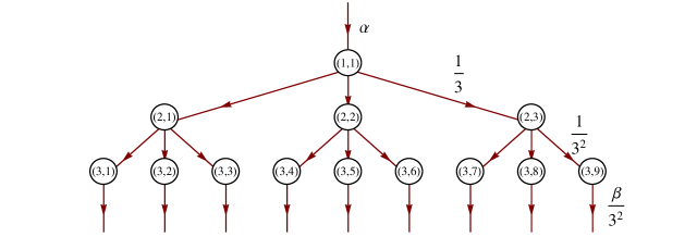
Figure 1: TASEP on a tree with $K=3$ and $b=3$. The notation for labelling sites is $\left(k,i\right)$; where $k$ labels the level in the tree and $i$ labels the site at that level. The number of sites at level $k$ is $b^{k-1}$. The hopping rates at each level are given on the right. The hopping rates are scaled so that the “total” hopping rate from one level to the next is unity and independent of $b$. The exit hopping rates at the final level are similarly scaled so that the “total” exit rate is $\beta$ independent of $b$. These “total” hopping rates are therefore identical to the one-dimensional case.

Basu and Mohanty [18] define hopping rates that significantly reduce the exclusion effect and lead to a “free flow” of particles to the exit boundary and rather straightforward behaviour. Here we take an alternative approach where the hopping rate is reduced by a factor of $\frac{1}{b}$ at each level, so that the hopping rate from a site at level $k$ to a connected site at level $k+1$ is $1/b^{k}$. The number of sites increases by a factor of $b$ at each level so that the “overall” hopping rate from one level to the next remains of the same order. At the exit boundary (level $K$) there are $b^{K-1}$ sites labelled $\left(K,i\right)$ with $i=1,\ldots,b^{K-1}$ . We give each site an exit rate $\beta/b^{K-1}$ so that the “overall” exit rate is of order $\beta$ . With this definition of the TASEP on a tree the overall entry rate is $\alpha$ and the overall removal rate is $\beta$ as in the normal one-dimensional TASEP. With $b=1$ the hopping rates reduces to the usual open TASEP model.

The dynamics can be summarised as follows. During every infinitesimal time interval $\mathrm{d}t$, each particle at a site $\left(k,i\right)$ with $1\leq k\leq K-1$ (i.e. bulk sites with $\tau_{k,i}=1$) will hop to an empty connected neighbour at level $k+1$ (i.e. neighbours with $\tau_{k+1,j}=0$) with probability $\mathrm{d}t/b^{k-1}$. During the same infinitesimal time interval, if site $\left(1,1\right)$ is empty ($\tau_{1,1}=0$) a particle is added with probability $\alpha\mathrm{d}t$ and any particle at level $K$ is removed with probability $\beta\mathrm{d}t/b^{K-1}$.

2.2 Steady-state current

The current of particles $j_{k,i}$ into a given site $\left(k,i\right)$ depends on the probability that the site is vacant, its downstream neighbour is occupied and the hopping probability. This leads to expressions for the average current into site $\left(k,i\right)$ in the bulk and at the two boundaries

$$j_{1,1} = \alpha\left(1-\left\langle\tau_{1,1}\right\rangle\right)$$ (1)

$$j_{k,i} = \frac{1}{b^{k-1}}\left\langle\tau_{k-1,\left\lceil\nicefrac{{i}}{{b}}\right\rceil}\left(1-\tau_{k,i}\right)\right\rangle$$ (2)

$$j_{K+1,i} = \frac{\beta}{b^{K-1}}\left\langle\tau_{K,i}\right\rangle$$ (3)

where $\left\lceil x\right\rceil$ is the ceiling function defined to be the smallest integer greater than or equal to $x$. The currents are time-dependent and the average is over a time-dependent probability distribution for the $\tau_{k,i}$ which is dependent on initial conditions. We are interested in the steady state where the system has evolved for long enough that all correlation functions are independent of time and all memory of initial conditions has been lost. In particular any asymmetry in the initial conditions will have been lost and from the symmetry of the lattice we have in steady state

$$\left\langle\tau_{k,i}\left(1-\tau_{k+1,bi-b+j}\right)\right\rangle\textnormal{is independent of}\,j\,\textnormal{for}\,1\leq j\leq b\textnormal{.}$$ (4)

If we define the total current $J_{k}$ flowing into level $k$ as $J_{k}=\sum_{i}j_{k,i}$ then in steady state we have

$$J_{1} = \alpha\left(1-\left\langle\tau_{1}\right\rangle\right)$$ (5)

$$J_{k} = \left\langle\tau_{k-1}\left(1-\tau_{k}\right)\right\rangle$$ (6)

$$J_{K+1} = \beta\left\langle\tau_{K}\right\rangle$$ (7)

where all the two-point correlation functions are between connected sites on adjacent levels in the tree and we have suppressed the site index $i$ on the $\tau_{k,i}$ because in steady state the average occupation number and the connected two point correlation function depend only on the level index, $k$. In steady state the average site occupancy is independent of time and therefore we expect the total current into each level to be the same steady-state current, $J=J_{k}$, independent of $k$. We can therefore obtain a set of equations for the expectation values by equating the right hand side of each of equation (5), (6)and (7). There is no explicit dependence on $b$ in these equations suggesting that the behaviour of the tree model will be the same as the one-dimensional case. However, as we show later, the higher level correlation functions do have an explicit dependence on $b$ leading to different behaviour from the one-dimensional model. The steady-state current equations are insufficient to determine the $\left\langle\tau_{k}\right\rangle$ without some approximation because of the coupling to higher level correlation functions.

2.3 Mean field theory

In the mean field approximation [4] we ignore correlations between sites and in particular take $\left\langle\tau_{k-1}\left(1-\tau_{k}\right)\right\rangle=t_{k-1}\left(1-t_{k}\right)$ where $t_{k}=\left\langle\tau_{k}\right\rangle$. If we substitute these in the total current equations (5), (6) and (7), and use the steady-state condition that current is constant we obtain the mean field theory equations

$$\alpha\left(1-t_{1}\right) = t_{1}\left(1-t_{2}\right)$$ (8)

$$t_{k-1}\left(1-t_{k}\right) = t_{k}\left(1-t_{k+1}\right)$$ (9)

$$t_{K-1}\left(1-t_{K}\right) = \beta t_{k}\,.$$ (10)

These are independent of $b$ so that at the level of mean field theory the model defined on the tree is formally identical to the one-dimensional case. Therefore at the mean field theory level all tree models considered in this paper will have the same phase diagram as the one-dimensional MFT phase diagram (see [4]) shown in figure 2. However, $t_{k}$ is the average occupancy of a site at level $k$ not the average occupancy of the level overall which grows exponentially.

As in the one-dimensional case there are three phases determined by the boundary hopping rates $\alpha$ and $\beta$. These are most easily understood in terms of the iteration of the MFT equations(8)(9) and (10) (see [4]). When the steady-state current $J<\frac{1}{4}$ there is a high density stable fixed point and a low density unstable fixed point with densities given by

$$t_{\pm}=\frac{1}{2}\left[1\pm\sqrt{1-4J}\right].$$

In the high density phase $\alpha>\beta$ and $\alpha<\frac{1}{2}$. The density rapidly converges to the stable high density fixed point and the current is given by $J=\beta\left(1-\beta\right)$. In the low density phase $\alpha<\beta$ and $\beta<\frac{1}{2}$. The initial density $t_{1}$ is set infinitesimally close to the unstable low density fixed point and only diverges from it as the exit boundary is approached. The steady-state current is given by $J=\alpha\left(1-\alpha\right)$.

In the maximal current phase $\alpha>\frac{1}{2}$ and $\beta>\frac{1}{2}$. The current is $J=\frac{1}{4}$ and there is a single marginal fixed point (there are no fixed points for $J>\frac{1}{4}$). The initial density $t_{1}$ is set above the marginal fixed point. The density rapidly approaches the fixed point but moves below it as the exit boundary is approached.

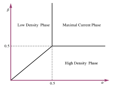
Figure 2: Mean field phase diagram for TASEP on a tree.

We have seen that at the mean field level the tree model is the same as the one-dimensional model. In the rest of the paper we will go beyond MFT and explore correlations. This will allow us to provide some results on the $b$ dependence of the correlation functions.

3 Dynamics and the master equation

As a next step to understanding the behaviour of the tree model we derive the exact equations of motion for the average occupation number, $\left\langle\tau_{k,i}\right\rangle$ and then look at the steady-state behaviour. This approach enables us to recover the results of Section 2 but has the advantage of being applicable to an arbitrary correlation function as we will show in Section 4.

3.1 Continuous time dynamics and the master equation

As a starting point for obtaining the equations of motion we use a master equation to describe the evolution of the the probability $P\left(\mathcal{C},t\right)$ of the system being in configuration $\mathcal{C}\equiv\left\{\tau_{k,i}\right\}$ at time $t$ given some set of initial conditions

$$\frac{\partial P\left(\mathcal{C},t\right)}{\partial t}=\sum_{\mathcal{C}^{\prime}}P\left(\mathcal{C}^{\prime},t\right)W\left(\mathcal{C}^{\prime}\rightarrow\mathcal{C}\right)-\sum_{\mathcal{C}^{\prime\prime}}P\left(\mathcal{C},t\right)W\left(\mathcal{C}\rightarrow\mathcal{C}^{\prime\prime}\right)$$ (11)

where the transition rates are defined by

$$W\left(\mathcal{C^{\prime}}\rightarrow\mathcal{C}\right)=\begin{cases}\alpha&\textrm{if }\mathcal{C}\,\textnormal{is identical to }\mathcal{C^{\prime}\,}\textnormal{except for an additonal particle at}\left(1,1\right)\textnormal{ }\\ \nicefrac{{\beta}}{{b^{K-1}}}&\textnormal{if $\mathcal{C^{\prime}\,}$is identical to $\mathcal{C}$\,}\textnormal{except for an additional particle at level }K\\ \nicefrac{{1}}{{b^{k}}}&\textnormal{if }\mathcal{C\,}\textnormal{and }\mathcal{C^{\prime}\,}\textnormal{differ on a single pair of connected sites }\left(k,i\right)\\ &\textnormal{and any one of }\left(k+1,bi-b+1\right),\ldots,\left(k+1,bi\right)\\ 0&\textnormal{otherwise.}\end{cases}$$ (12)

With this definition for the transition rates we have precisely the dynamics we defined in section 2.

3.2 Exact equations for the time evolution of the average site density

The equation of motion for the expectation value of the occupation number, $\left\langle\tau_{k,i}\right\rangle$, is given by

$$\frac{\partial\left\langle\tau_{k,i}\right\rangle}{\partial t}=\sum_{\mathcal{C}^{\prime}}P\left(\mathcal{C}^{\prime},t\right)\sum_{C\neq C^{\prime}}\tau_{k,i}W\left(\mathcal{C}^{\prime}\rightarrow\mathcal{C}\right)-\sum_{\mathcal{C}}P\left(\mathcal{C},t\right)\tau_{k,i}\sum_{C^{\prime\prime}}W\left(\mathcal{C}\rightarrow\mathcal{C}^{\prime\prime}\right)$$

where we have used the master equation (11) and taken $\mathcal{C}\equiv\left\{\tau_{k,i}\right\}$ , so that configuration $\mathcal{C}$ determines the values of $\tau_{k,i}$. Substituting for the transition rates from equation (12) gives three equations for the time evolution of the average occupation number in terms of two-point correlation functions

$$\frac{\partial\left\langle\tau_{1,1}\right\rangle}{\partial t} = \alpha\left(1-\left\langle\tau_{1,1}\right\rangle\right)-\frac{1}{b}\sum_{i=1}^{b}\left\langle\tau_{1,1}\left(1-\tau_{2,i}\right)\right\rangle$$ (13)

$$\frac{\partial\left\langle\tau_{k,i}\right\rangle}{\partial t} = \frac{1}{b^{K-1}}\left\langle\tau_{k-1,\left\lceil\nicefrac{{i}}{{b}}\right\rceil}\left(1-\tau_{k,i}\right)\right\rangle-\frac{1}{b^{k}}\sum_{j=0}^{b-1}\left\langle\tau_{k,i}\left(1-\tau_{k+1,bi-j}\right)\right\rangle$$ (14)

$$\frac{\partial\left\langle\tau_{K,j}\right\rangle}{\partial t} = \frac{1}{b^{K-1}}\left\langle\tau_{K-1,\left\lceil\nicefrac{{j}}{{b}}\right\rceil}\left(1-\tau_{K,j}\right)\right\rangle-\frac{\beta}{b^{K-1}}\left\langle\tau_{K,j}\right\rangle$$ (15)

where $1\leq i\leq b^{k-1}$ in the second equation and $1\leq j\leq b^{K-1}$ in the third equation.

3.3 Steady-state equations of motion

In steady state any asymmetry in the initial conditions will have been lost and from the symmetry of the lattice the steady-state form of equations (13), (14) and (15) is

$$0 = \alpha\left(1-\left\langle\tau_{1}\right\rangle\right)-\left\langle\tau_{1}\left(1-\tau_{2}\right)\right\rangle$$ (16)

$$0 = \left\langle\tau_{k-1}\left(1-\tau_{k}\right)\right\rangle-\left\langle\tau_{k}\left(1-\tau_{k+1}\right)\right\rangle$$ (17)

$$0 = \left\langle\tau_{K-1}\left(1-\tau_{K}\right)\right\rangle-\beta\left\langle\tau_{K}\right\rangle$$ (18)

where all the two-point correlation functions are between connected sites on adjacent levels in the tree and we have suppressed the site index. The lattice symmetry that is used here is that the steady-state equations are invariant under transformations of the lattice that preserve the connectivity of the tree. For example, any two sub branches that have their “root” at the same site can be interchanged without changing the steady-state equations.

These are identical to the total steady-state current equations (5), (6) and (7), obtained using the assumption of constant current. They are also the same as the one-dimensional TASEP equations. However, the master equation approach used in this section is more easily extended to higher-order correlation functions.

4 Correlation functions

We now consider the equation of motion for a general correlation function. In the case of a TASEP where $\tau_{i}$ can only take the values one or zero the most general correlation function is

$$c\left(S,t\right)\equiv\left\langle\prod_{i\in S}\tau_{i}\right\rangle\equiv\sum_{\mathcal{C}}P\left(\mathcal{C},t\right)\prod_{i\in S}\tau_{i},$$ (19)

where $S$ is any given subset of sites in the lattice. In appendix A we derive the equation of motion for $c\left(S,t\right)$ for the TASEP on an arbitrary lattice. In this section we will use this for correlation functions on the tree.

4.1 Time evolution equation for tree lattice

We would like to generalise the steady-state equations (16), (17) and (18) to the general correlation function (19). In appendix A we consider a general open TASEP on an arbitrary network and obtain the equation of motion for the correlation functions; equation (68) . The steady-state form of this for a subset of sites $S$ on a tree is

$$0 = \alpha\left\{c\left(S\left[\overline{\left(1,1\right)}\right]\right)-c(S)\right\}\delta\left[\left(1,1\right)\in S\right]$$ (20)

$$+ \sum_{\left(i,j\right)\in S_{in}}\frac{1}{b^{i-1}}\left\{c\left(S\left[\left(i-1,\left\lceil\nicefrac{{j}}{{b}}\right\rceil\right),\overline{\left(i,j\right)}\right]\right)-c\left(S\left[\left(i-1,\left\lceil\nicefrac{{j}}{{b}}\right\rceil\right)\right]\right)\right\}$$

$$- \sum_{\left(i,j\right)\in S_{out}}\frac{1}{b^{i}}\sum_{(i+1,k)\in O\left(i,j\right)}\left\{c(S)-c\left(S\left[\left(i+1,k\right)\right]\right)\right\}$$

$$- \frac{\beta}{b^{K-1}}\sum_{i\in S_{exit}}c(S)$$

where we have discarded the $t$ dependence of the correlation function in (19) and the $\delta[\textrm{statement}]$ is a generalised Kronecker delta (or indicator function); equal to unity if statement is true and zero otherwise. The notation $S\left[\overline{\left(1,1\right)}\right]$ means the subset of sites obtained by removing site $\left(1,1\right)$ from the set of sites $S$. Similarly, $S\left[\left(i,k\right)\right]$ means the subset of sites obtained by adding site $\left(i,k\right)$ to $S$ and $S\left[\left(i,k\right),\overline{\left(j,l\right)}\right]$ means the subset of sites obtained by adding site $\left(i,k\right)$ to $S$ and removing site $\left(j,l\right)$. The various subsets of $S$ ($S_{entry}$, $S_{exit}$, $S_{in}$, $S_{out}$) that appear in the sums are defined in table 1. The outgoing neighbour set $O\left(i\right)$ and the incoming neighbour set $I\left(j\right)$ are also defined in table 1.

Subsets	Definition of boundary sites related to $S$.
$S_{entry}$	The subset of $S$ at which particles can enter $S$ from outside the lattice.
$S_{exit}$	The subset of $S$ at which particles can leave $S$ and exit the lattice.
$S_{in}$	The subset of $S$ where particles can enter $S$ from lattice sites that are not in $S$.
$S_{out}$	The subset of $S$ where particles can leave $S$ to sites in the lattice that are not in $S$.
$O\left(i\right)$	The set of outgoing neighbours to site $i\in S_{out}$ that are not in $S$.
$I\left(j\right)$	The set of incoming neighbours to site $j\in S_{in}$ that are not in $S$.

Table 1: Definition of subsets of boundary sites related to $S$

We see that the steady-state equations (16), (17) and (18) that relate the single-point correlation functions to the two-point correlation functions are the first in a hierarchy of equations. However, the branching ratio $b$ drops out of the lowest order equation leading to a mean field theory that is independent of $b.$ We see that this is not the case for other levels in the hierarchy and so any corrections to mean field theory should be dependent on $b$.

4.2 Exact solution when $\alpha+\beta=1$

An interesting question is whether mean field theory is exact in some situations. This would require a solution of the form

$$c(S)=\prod_{\left(k,j\right)\in S}t_{k}$$ (21)

for all possible $S$ where $t_{k}$ satisfies the mean field equations (8), (9) and (10). It is easy to show that where $S$ contains just a single site this equation is satisfied on the line $\beta=1-\alpha$ with $t_{k}=\alpha$, but we need to demonstrate this for any $S$. We take $\beta=1-\alpha$ and substitute the ansatz

$$c(S)=\alpha^{\left|S\right|}$$ (22)

into equation (20). This becomes

$$0 = \alpha^{\left|S\right|}\left(1-\alpha\right)\delta\left[\left(1,1\right)\in S\right]$$ (23)

$$+ \alpha^{\left|S\right|}\left(1-\alpha\right)\sum_{\left(i,j\right)\in S_{in}}\frac{1}{b^{i-1}}$$

$$- \alpha^{\left|S\right|}\left(1-\alpha\right)\sum_{\left(i,j\right)\in S_{out}}\frac{1}{b^{i}}\sum_{(i+1,k)\in O\left(i,j\right)}$$

$$- \frac{\alpha^{\left|S\right|}\left(1-\alpha\right)}{b^{K-1}}\sum_{i\in S_{exit}}.$$

We can eliminate the common factor to obtain

$$0 = \delta\left[\left(1,1\right)\in S\right]+\sum_{\left(i,j\right)\in S_{in}}\frac{1}{b^{i-1}}-\sum_{\left(i,j\right)\in S_{out}}\frac{1}{b^{i}}\sum_{(i+1,k)\in O\left(i,j\right)}1-\sum_{i\in S_{exit}}1.$$ (24)

This depends only on the properties of the lattice and not on the value of $\alpha$. We provide an inductive proof that it is satisfied for any $S$ in appendix B. This result is independent of $b$ and shows that the one-dimensional result [4] generalises to the tree.

4.3 Expansion of correlation functions in $1/b$ and mean field theory

There is another more general situation where mean field theory is exact; this is in the limit $b\rightarrow\infty$. First we shall give a simple heuristic argument for the result and then outline the proof. There are no closed loops in the tree so that in general neighbouring sites are correlated because the probability of hopping from a site at level $k$ is reduced if its neighbours at level $k+1$ are occupied. However, for a given site, as the number of these downstream nearest neighbour sites increases the effect of any single downstream nearest neighbour site will diminish and we expect that as $b\rightarrow\infty$ this mechanism eliminates any correlation between pairs of connected sites. We can put this plausibility argument on a more rigorous footing by considering an expansion of the correlation function in terms of $1/b$.

The correlation functions that we defined as

$$c\left(S\right)\equiv\left\langle\prod_{\left(k,i\right)\in S}\tau_{k,i}\right\rangle$$ (25)

are dependent on $b,$ so we can expand $c\left(S\right)$ as a power series in $1/b$

$$c\left(S\right)=\sum_{r=0}^{\infty}c_{r}\left(S\right)\frac{1}{b^{r}}$$ (26)

where the coefficients $c_{r}\left(S\right)$ are independent of $b$. Our hypothesis is that for a fixed choice of $S$, as $\frac{1}{b}\rightarrow 0$, the correlation function should satisfy mean field theory. This requires the zeroth order term to satisfy

$$c_{0}\left(S\right)=\prod_{k=1}^{K}t_{k}^{\left|S\left(k\right)\right|}$$ (27)

where $\left|S\left(k\right)\right|$ is the number of sites in $S$ at level $k$ of the tree and the $t_{k}$ satisfy the mean field equations (8), (9) and (10). In order to obtain this result we substitute the expansion (26) in (20). Retaining only the lowest order terms in $1/b$ gives

$$0 = \alpha\left|S\left(1\right)\right|\left\{c_{0}\left(S\left[\overline{\left(1,1\right)}\right]\right)-c_{0}\left(S\right)\right\}$$ (28)

$$+ \sum_{\left(i,j\right)\in S_{in}}\frac{1}{b^{i-1}}\left\{c_{0}\left(S\left[\left(i-1,\left\lceil\nicefrac{{j}}{{b}}\right\rceil\right),\overline{\left(i,j\right)}\right]\right)-c_{0}\left(S\left[\left(i-1,\left\lceil\nicefrac{{j}}{{b}}\right\rceil\right)\right]\right)\right\}$$

$$- \sum_{\left(i,j\right)\in S_{out}}\frac{1}{b^{i}}\sum_{(i+1,k)\in O\left(i,j\right)}\left\{c_{0}\left(S\right)-c_{0}\left(S\left[\left(i+1,k\right)\right)\right]\right\}$$

$$- \frac{\beta}{b^{K-1}}\left|S\left(K\right)\right|c_{0}\left(S\right)$$

We would like to extract the lowest power of $\frac{1}{b}$ with a non-zero coefficient. This is determined by the sites in $S$ that are closest to the root of the tree (i.e. site $\left(1,1\right)$). We must consider four different scenarios (note that $S$ can have any structure further away from the root)

• Scenario 1; $S$ contains $\left(1,1\right)$ so that $\left(1,1\right)$ is the site closest to the root,

• Scenario 2; $S$ contains a single bulk site that is closest to the root,

• Scenario 3; $S$ contains multiple bulk sites that are closest to the root, and

• Scenario 4; $S$ only contains sites at level $K$.

In scenario 1 the only terms that can contribute at zeroth order are

$$0=\alpha\left\{c_{0}\left(S\left[\overline{\left(1,1\right)}\right]\right)-c_{0}\left(S\right)\right\}-\lim_{b\rightarrow\infty}\frac{1}{b}\sum_{(2,j)\in O\left(1,1\right)}\left\{c_{0}\left(S\right)-c_{0}\left(S\left[\left(2,j\right)\right]\right)\right\}$$ (29)

where the sum in the second term is over the level $2$ sites not in $S$. The number of such sites is of order $b$ so the limit is required to extract the contribution at zeroth order. Notice that all structure in $S$ beyond level 2 has no effect on the correlation function.

If we now substitute the mean field hypothesis (27) we get

$$0=\alpha\left(1-t_{1}\right)-t_{1}\left(1-t_{2}\right)\lim_{b\rightarrow\infty}\left(\frac{b-\left|S\left(2\right)\right|}{b}\right).$$ (30)

Using the fact that $\left|S\right|$ is independent of $b$, we find that the mean field hypothesis is exact in the limit $b\rightarrow\infty$ and we recover the first boundary mean field equation (8). Therefore (8) is valid for any correlation function that contains the first site in the limit of large $b$.

In scenario 2 we assume that $S$ has a single site at level $l$ that is closest to the root. Equivalently

$$\left|S\left(k\right)\right|=0\textnormal{ for }k<l\textnormal{ and }\left|S\left(l\right)\right|=1$$

with the structure of $S$ arbitrary for $k>l$. We will assume without loss of generality that the site at level $l$ is $\left(l,1\right)$. In this case (28) becomes

$$0=\left\{c_{0}\left(S\left[\left(l-1,1\right),\overline{\left(l,1\right)}\right]\right)-c_{0}\left(S\left[\left(l-1,1\right)\right]\right)\right\}-\lim_{b\rightarrow\infty}\frac{1}{b}\sum_{\left(l+1,j\right)\in O\left(l,1\right)}\left\{c_{o}\left(S\right)-c_{0}\left(S\left[\left(l+1,j\right)\right]\right)\right\}$$ (31)

where the sum in the second term is over all downstream neighbours of $\left(l,1\right)$ that are not in $S$. Again the correlation function does not depend on the structure of $S$ beyond the first two occupied levels of the tree. If we now substitute the mean field hypothesis (27) we get

$$0=\left\{t_{l-1}\prod_{k=l+1}^{K}t_{k}^{\left|S\left(k\right)\right|}-t_{l-1}\prod_{k=l}^{K}t_{k}^{\left|S\left(k\right)\right|}\right\}-\left\{\prod_{k=l}^{K}t_{k}^{\left|S\left(k\right)\right|}-t_{l+1}\prod_{k=l}^{K}t_{k}^{\left|S\left(k\right)\right|}\right\}\lim_{b\rightarrow\infty}\left(\frac{b-\left|O\left(l,1\right)\right|}{b}\right).$$ (32)

Taking the $b\rightarrow\infty$ limit we find that mean field theory is exact and assuming that none of the $t_{k}$ are zero we recover the bulk mean field equation (9). We have therefore shown that to zeroth order in $\frac{1}{b}$ any correlation function with a single site nearest the root satisfies mean field theory exactly. Scenario 3 is a straightforward extension of this analysis and shows that this conclusion holds even if we allow multiple sites at level $l$.

In scenario 4 we assume that $S$ only includes sites at level $K$. In this case equation (28) reduces to

$$0=\left\{c_{0}\left(S\left[\left(K-1,1\right),\overline{\left(K,1\right)}\right]\right)-c_{0}\left(S\left[\left(K-1,1\right)\right]\right)\right\}-\beta c_{0}\left(S\right).$$ (33)

Substituting the mean field hypothesis (27) satisfies this equation and recovers the second boundary mean field theory equation (10).

In summary, we find that mean field theory is exact when we consider a fixed correlation function and let $b\rightarrow\infty$. We expect that mean field theory will be an increasingly good approximation as the branching number increases. This bears out the plausibility argument given at the start of the section and it seems reasonable to expect to be true on other types of lattices and for more complex exclusion processes. That is, mean field theory becomes an increasingly good approximation as the branching number or coordination number is increased for any “TASEP on a network” model where loops are not significant.

As a step beyond mean field theory we would like to look at $\frac{1}{b}$ corrections to the the correlation function expansion in equation (26). Unfortunately this has proved much more difficult than we originally hoped. At zeroth order we found that all correlation functions can be expressed in terms of a single site function $t_{k}$ using equation (27). It might be expected that to first order in the expansion in $\frac{1}{b}$ we would have an analogous result but with two site correlation functions (or at least a limited set of short range correlation functions) replacing the single site functions. Indeed we do find that an arbitrary correlation function can be expressed in terms of a reduced set of correlation functions, but the reduced set is not limited to short range correlation functions and in fact includes correlation functions that extend across all layers of the tree. We have been unable to find an analytic approach to dealing with this complexity and have chosen instead to make a first step by solving the two level tree in the next section. We address larger trees using Monte-Carlo simulation in Section 6.

5 Analytical study of the two level tree

In this section we make a full analysis for the case $K=2$ or two level tree. As we shall see this is not a trivial problem to solve for arbitrary $b$. We derive recursion relations for the correlation functions, then first show how to obtain a $1/b$ expansion solution to these. Then for the case $\alpha=1$ we obtain the exact solution of the recursion recursion relations as a finite sum. We show how to write this solution in an integral representation that easily allows the $1/b$ expansion to be recovered by the saddle point method.

5.1 Recursion relations for the two level tree

Our starting point is to use the symmetry of the lattice to simplify the correlation function $c_{S}$. In steady state $c_{S}$ will be invariant under the exchange of any sub-branches of the tree. In the $K=2$ case this means that any $c_{S}$ that has $m$ sites at level 2 is identical. As a consequence we can define

$$c_{S}=c\left(l,m\right)$$ (34)

where $l=0\,\textrm{or}\,1$ indicates whether site $\left(1,1\right)$ is included in the correlation function and $m=0,1,\ldots,b$ is the number of sites included at level 2.

In the case $K=2$ and $l=1$ the steady state equation (20) becomes

$$0=\alpha c(0,m)-\left(1+\alpha+\frac{m}{b}\left(\beta-1\right)\right)c\left(1,m\right)+\left(1-\frac{m}{b}\right)c\left(1,m+1\right)\quad\mbox{for}\quad m\geq 0\,.$$ (35)

In the case $l=0$ the steady state equation gives

$$0=c\left(1,m-1\right)-c\left(1,m\right)-\beta c\left(0,m\right)\quad\mbox{for}\quad m\geq 1$$ (36)

with boundary condition $c(0,0)=1$.

We may eliminate $c(0,m)$ from (35, 36) to obtain

$$0=\frac{\alpha}{\beta}c(1,m-1)-\left(\frac{\alpha+\beta+\alpha\beta}{\beta}+\frac{m}{b}\left(\beta-1\right)\right)c\left(1,m\right)+\left(1-\frac{m}{b}\right)c\left(1,m+1\right)\quad\mbox{for}\quad m\geq 1\,.$$ (37)

Finally, the boundary case $m=0$ of (35) yields

$$0=\alpha-(1+\alpha)c(1,0)+c(1,1)\;.$$ (38)

5.2 $1/b$ expansion for a two level tree

In the limit $b\rightarrow\infty$ we can solve these recursion relations easily to obtain

$$c\left(0,m\right) = t_{2}^{m},$$ (39)

$$c\left(1,m\right) = t_{1}t_{2}^{m},$$ (40)

where $t_{1}$ and $t_{2}$ are the same as the solutions to the mean field theory equations (8), (9) and (10). They are given by

$$t_{1}=1-\frac{\alpha+\beta+\alpha\beta-\sqrt{\left(\alpha+\beta+\alpha\beta\right)^{2}-4\alpha\beta}}{2\alpha}$$ (41)

$$t_{2}=\frac{\alpha+\beta+\alpha\beta-\sqrt{\left(\alpha+\beta+\alpha\beta\right)^{2}-4\alpha\beta}}{2\beta}\,.$$ (42)

We can develop an expansion around these mean field results by expanding $c\left(l,m\right)$ as a power series in $\frac{1}{b}$ of the form

$$c\left(l,m\right)=\sum_{r=0}^{\infty}c_{r}\left(l,m\right)\frac{1}{b^{r}}$$ (43)

where $c_{0}\left(l,m\right)$ is given by the mean field results (40) and (40). Substituting this expansion into equation (35) and equating successive powers of $\frac{1}{b}$ gives a sequence of recursion relations that may be solved to obtain the coefficients in equation (43).

As an illustration we give order $\frac{1}{b}$ correction

$$c\left(1,m\right) = t_{1}t_{2}^{m}+\frac{1}{b}\,\frac{\alpha\beta\left(\beta-1+t_{2}\right)t_{2}^{m+1}}{2\left(\alpha+1-t_{2}\right)^{2}\left(\beta t_{2}^{2}-\alpha\right)^{2}}\Bigl{\{}\left(\alpha+1-t_{2}\right)m^{2}$$ (45)

$$-\left(\alpha+\beta t_{2}^{2}\right)\left(\alpha+1-t_{2}\right)m-2\alpha t_{2}\Bigl{\}}+\mathcal{O}\left(\frac{1}{b^{2}}\right)\,.$$

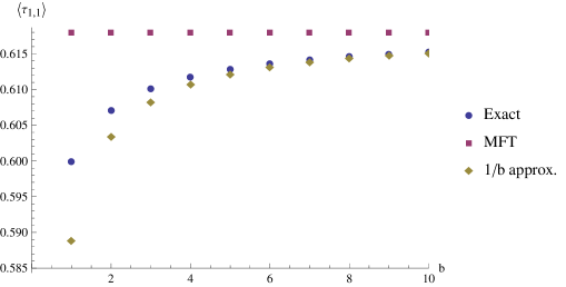
Figure 3: Comparison of exact value of $\left\langle\tau_{1,1}\right\rangle$against mean field and $\frac{1}{b}$ corrections for two level tree with $\alpha=\beta=1$. The blue circles are the exact values from solving the recursion relation for a given value of $b$, the dashed line is the mean field estimate which is independent of $b$ and the red squares are the result of expansion to $\mathcal{O}(\frac{1}{b})$ in equation (45).

This can be used to approximate the average occupation number of the first site $\left\langle\tau_{1,1}\right\rangle=c\left(1,0\right)$ for any value of $b$. This is plotted in figure 3 and compared with the mean field theory estimate and exact results obtained by solving the recursion relations exactly for small values of $b$. The approximation is excellent for values of $b>5$.

This $1/b$ expansion approach is effective, but we have implicitly made assumptions about the $b$ dependence of $c\left(l,m\right)$ in order to make the $1/b$ expansion of the recursion relation (35). We address this in the next section using an alternative approach that confirms that the procedure does give correct results when $m\sim\mathcal{O}$$\left(1\right)$.

5.3 Exact finite sum expressions for correlation functions of two level tree

In the case $\beta=1$ we can obtain a simple full exact solution of the two level tree in the form of a finite sum. In the case $\beta=1$, (37) becomes

$$0=c(1,m-1)-\left(\frac{2\alpha+1}{\alpha}\right)c\left(1,m\right)+\frac{1}{\alpha}\left(1-\frac{m}{b}\right)c\left(1,m+1\right)\quad\mbox{for}\quad m\geq 1$$ (46)

We now change index to $n=b-m$ to express (35) in the form of a recursion “down” from $b$ rather than “up” from $0$. Defining $D\left(n\right)=c\left(1,b-n\right)=c\left(1,m\right)$ equation (46) becomes

$$D\left(n+1\right)=a\,D\left(n\right)-\frac{n}{b\alpha}D\left(n-1\right)$$ (47)

for $n=0,1,\ldots b-1$, where

$$a=\frac{2\alpha+1}{\alpha}.$$ (48)

The first few terms in this recursion are easy to compute

$$D(1) = aD(0)$$

$$D(2) = \left(a^{2}-\frac{1}{b\alpha}\right)D(0)$$

$$D(3) = \left(a^{3}-\frac{3a}{b\alpha}\right)D(0)$$

$$D(4) = \left(a^{4}-\frac{6a^{2}}{b\alpha}+\frac{3}{(b\alpha)^{2}}\right)D(0)$$

$$\vdots$$

It can be proven by induction that the general solution for $D(n)$ is of the form

$$D\left(n\right)=\sum_{r=0}^{\left\lfloor\frac{n}{2}\right\rfloor}\left(-1\right)^{r}\frac{a^{n-2r}}{\left(\alpha b\right)^{r}}\left(2r-1\right)!!\binom{n}{2r}\,D\left(0\right)$$ (49)

where $\left(2r-1\right)!!=(2r-1)(2r-3)\cdots 1$ with the convention $\left(-1\right)!!=1$ and $\left\lfloor x\right\rfloor$ is the floor function defined to be the largest integer less than or equal to $x$.

Returning to the correlation function notation we have

$$c\left(1,m\right)=c\left(1,b\right)S_{m}$$ (50)

where

$$S_{m}=\sum_{p=0}^{\left\lfloor\frac{b-m}{2}\right\rfloor}a^{b-m-2p}\left(\frac{-1}{\alpha b}\right)^{p}\binom{b-m}{2p}\left(2p-1\right)!!\,.$$ (51)

Finally to fix $c\left(1,b\right)$ we use the boundary condition equation (38) to obtain

$$c(1,b)=\frac{\alpha}{(1+\alpha)S_{0}-aS_{1}}\;.$$ (52)

We may now write the exact solution for the correlation functions as

$$c\left(1,m\right) = \frac{\alpha S_{m}}{\left(\alpha+1\right)S_{0}-S_{1}}$$ (53)

$$c\left(0,m\right) = \frac{\alpha\left(S_{m-1}-S_{m}\right)}{\left(\alpha+1\right)S_{0}-S_{1}}\;.$$ (54)

Thus equations (53,54) give exact finite sum expressions for all correlation functions for any $b$.

5.4 Saddle-point expansion of exact solution

We would like to obtain an asymptotic expansion in $1/b$ as in Section 5.2 from expressions (53,54). However the binomial term involving $b$ in equation (51) means that we do not yet have the required form. To obtain an asymptotic form we first introduce an integral representation of the double factorial (which may be verified by integration by parts)

$$\left(2p-1\right)!!=\frac{2^{p}}{\sqrt{\pi}}\intop_{-\infty}^{\infty}\mathrm{d}u\,u^{2p}e^{-u^{2}}\;.$$ (55)

Substituting into (51) this gives

$$S_{m} = \frac{a^{b-m}}{\sqrt{\pi}}\int_{-\infty}^{\infty}\mathrm{d}u\,e^{-u^{2}}\sum_{\begin{array}[]{c}p=0\\ p\mathrm{\,even}\end{array}}^{\infty}\left[\frac{iu\sqrt{2}}{a\sqrt{\alpha b}}\right]^{p}\binom{b-m}{p}\;.$$

The series can be summed and with a change of variable $v=1+\frac{iu\sqrt{2}}{a\sqrt{\alpha b}}$ we can express $S_{m}$ as an integral in the form

$$S_{m}=\frac{a^{b-m+1}\sqrt{\alpha b}}{i\sqrt{2\pi}}\int_{-i\infty}^{i\infty}\mathrm{d}v\,\frac{1}{v^{m}}\exp bg(v)\,.$$ (57)

where

$$g(v)=\frac{a^{2}\alpha}{2}\left(v-1\right)^{2}+\ln v\,.$$ (58)

We can obtain an asymptotic expansion in $b$ using steepest descents, but we need to make some assumptions about the behaviour of $m$. We consider three regimes;

(i)

Assume $m\sim\mathcal{O}\left(1\right)$. This is the case of most practical interest; where the correlation function has a fixed number (of order 1) of sites. It corresponds to the assumptions we made in Section 4.3 to show that MFT is exact in the $b\rightarrow\infty$ limit. It also enables the computation of density and current.

(ii)

Assume $\frac{m}{b}=d$ where $d\sim\mathcal{O}\left(1\right)$ and $0<d<1$. This corresponds to correlation functions with a finite proportion of the total number of sites.

(iii)

Assume $b-m=n$ where $n\sim\mathcal{O}\left(1\right)$. This corresponds to correlation functions containing nearly all sites.

We address regime (i) first and take $b\gg 1$ and $m\sim\mathcal{O}\left(1\right)$. We can use steepest descents to obtain an asymptotic expansion in $b$ from equation (57). In this regime the pre-factor $1/v^{m}$ is independent of $b$ and the stationary points for the steepest descents are determined by $g\left(v\right)$ in equation (58). This has stationary points

$$v_{\pm}=\frac{1}{2}\left\{1\pm\left(1-\frac{4}{\alpha a^{2}}\right)^{\nicefrac{{1}}{{2}}}\right\}$$ (59)

and they are shown in figure 4. We see that the $\ln v$ term in equation (58) leads to a branch cut along the negative real axis and a logarithmic singularity at the origin. In order to use the saddle point approximation we deform the contour in equation (57) away from the imaginary axis to run through one of the stationary points. This will not succeed for the $v_{-}$ stationary point because the path of steepest descents runs along the real axis towards the origin and there is no return path through low values of the integrand. With $v_{+}$ the path of steepest descent is parallel to the imaginary axis and the contour can easily be chosen so that only points close to the saddle point contribute to the integral.

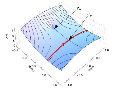
Figure 4: Plot of the real part of $g\left(v\right)$ (see equation (58)) in the complex plane indicating its two stationary points $v_{\pm}$. The physically relevant stationary point is $v_{+}$.

Using this contour we find that the zeroth order term in the asymptotic expansion is given by

$$c\left(1,m\right)\sim\frac{\alpha}{1+\alpha-\frac{1}{av_{+}}}\left(av_{+}\right)^{-m}$$ (60)

If we compare equation (42) with equation (59) for $\beta=1$ we see that $t_{2}=1/(av_{+})$ and with a little algebra we see that equation (60) is equivalent to the MFT result equation (40). In general the saddle point is equivalent to MFT. This is in agreement with the results of Section 4.3 where we showed that the MFT results become exact if we take a fixed correlation function and then take the large $b$ limit. Further note that the same mean field theory and saddle point hold for $m\ll b$ i.e. $m=o\left(b\right)$.

We can extend the asymptotic expansion to higher order. One can compute the correction to the saddle point and one recovers the second term in the expansion (45). Similarly by computing higher order corrections to the saddle point we can in principle compute the full asymptotic expansion. For example with $\alpha=1$ and $m=0$ we obtain

$$c\left(1,0\right)=0.618034-\frac{0.0291796}{b}+\frac{0.0238699}{b^{2}}-\frac{0.032957}{b^{3}}+O\left(\left(\frac{1}{b}\right)^{4}\right).$$ (61)

This result agrees with the first order correction given in equation (45). This result is used in figure 5 to plot the steady-state current using the relationship $J=\alpha\left(1-c\left(1,0\right)\right)$. With the exception of $b=1$ additional terms improve the approximation, but provide little improvement over the first order correction above $b=5$.

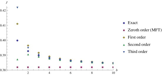
Figure 5: The steady-state current $J$ versus $b$ for a two level tree ($K=2$) for $\alpha=\beta=1$. The exact results are obtained by numerical solution of the steady-state equation (20). The approximate values are obtained from the asymptotic expansion of equation (57) about $v_{+}$. The zeroth order term is equivalent to MFT. The first order result includes only the order $1/b$ term. Including second and third order terms in $1/b$ gives improved accuracy for small values of $b$, but provide little improvement above $b=5$.

We now turn to the other two regimes for $m.$ In regime (ii) with $d=b/m$ we write equation (57) and equation (58) as

$$S_{m}=\frac{a^{b-m+1}\sqrt{\alpha b}}{i\sqrt{2\pi}}\int_{-i\infty}^{i\infty}\mathrm{d}v\,\exp bg_{d}(v).$$ (62)

and

$$g_{d}(v)=\frac{a^{2}\alpha}{2}\left(v-1\right)^{2}+\left(1-d\right)\ln v.$$ (63)

The steepest descents contour now passes through one of the stationary points of $g_{d}\left(v\right)$ which are given by

$$v_{d}^{\pm}=\frac{1}{2}\left\{1\pm\left(1-\frac{4\left(1-d\right)}{\alpha a^{2}}\right)^{\nicefrac{{1}}{{2}}}\right\}.$$ (64)

Following a similar argument to regime (i), the contour of integration runs parallel to the imaginary axis and passes through $v_{d}^{+}$ and an asymptotic expansion can be obtained using steepest descents. The zeroth order term is

$$c\left(1,m\right)=\frac{\alpha a^{-bd}}{1+\alpha-\frac{1}{av_{+}}}\sqrt{\frac{g^{{}^{\prime\prime}}\left(v_{+}\right)}{g_{d}^{{}^{\prime\prime}}\left(v_{d}^{+}\right)}}\exp\left\{b\left(g_{d}\left(v_{d}^{+}\right)-g\left(v^{+}\right)\right)\right\}.$$ (65)

Finally, in regime (iii), the same type of analysis can be repeated to obtain a slightly simpler form

$$c\left(1,m\right)=\frac{\alpha a^{n-b-1}}{1+\alpha-\frac{1}{av_{+}}}\sqrt{\frac{g^{{}^{\prime\prime}}\left(v_{+}\right)}{\alpha}}\exp\left\{-bg\left(v^{+}\right)\right\}.$$ (66)

The $m$ dependence is a simple exponential through the parameter $n$. In figure 6 we plot the three zeroth order asymptotic expansions for $c\left(1,m\right)$ versus the exact values. We see that in regime (i) (small $m$) equation (60) provides a good approximation to the exact results and in regime (iii) ($m$ close to $b$) equation (66) provides a good approximation to the exact results. In addition, we see that equation (65) actually gives an excellent fit in all three regimes. This is not surprising since equation (65) reduces to equation (60) in regime (i) and equation (66) in regime (iii).

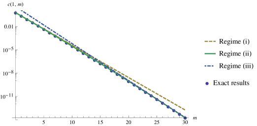
Figure 6: Comparison of the three regimes of the asymptotic expansion for the correlation function $c\left(1,m\right)$ with $b=30$ and $\alpha=\beta=1$. The exact results are from equation (53), regime (i) is given by equation (60), regime (ii) is given by equation (65) and regime (iii) is given by equation (66).

6 Simulation results

In order to investigate trees with $K>2$ with finite $b$ we used Monte Carlo simulation. We simulated the system using a variant of the waiting time algorithm [22] optimized for best performance for our specific model. The state of the system was described by a sequence $\{\tau_{k,i}\}$ of occupation numbers (0 or 1), and a vector $\{n_{k}\}$ of the numbers $n_{k}$ of particles in level $k$ that can jump to (free) sites in level $k+1$. Although $\{\tau_{k,i}\}$ would suffice to fully define a microstate, the use of the redundant vector $\{n_{k}\}$ improved the speed of the algorithm. Namely, in each time step we calculated total rates $\{r_{k}=n_{k}/b^{k}\}$ of hopping from level $k$ to $k+1$ based on $n_{k}$, and then used these to choose the level from which the hop would be attempted. The selection was made by scanning through the list of all $K+1$ rates (including the hop into the root with rate $\alpha(1-\tau_{1,1})$, and the hop out the lattice with rate $\beta n_{K}/b^{K-1}$), and since there were always not more than $K\leq 20$ levels, this approach was much faster than if we had just tried to pick up the departure site directly out of $1+b+b^{2}+\dots+b^{K-1}$ possibilities. After selecting the level $k$, the program chose an occupied site $i$ from this level and one of its empty neighbours $j$ from the next level (by trial and error), and updated the variables $\{\tau_{k,i}\}$ and $\{n_{k}\}$, i.e., the particle jumped from $(k,i)$ to $(k+1,j)$. Finally, the program increased the time by an exponentially-distributed random variable $\Delta t$ with mean $1/R_{{\rm tot}}$, where $R_{{\rm tot}}$ was the sum of all rates.

Before any data were collected, the program performed a “thermalization run” for 10% of the total simulation time. Then, the program accumulated the histogram of the density profile and the current every $N/2$ steps, weighting each of them by $\Delta t$. Each simulation was repeated 10 times, starting each time from a different seed for the random number generator to ensure statistical independence, and errors of $\left<\tau_{k,i}\right>$ and $\left<J\right>$ were estimated as standard errors.

To explore the behaviour of the TASEP on a tree for $K>2$ we have used Monte Carlo simulations for system sizes up to 6 million sites. The exponential growth in the system size with $K$, the number of layers in the tree, limits the depth of tree we can easily simulate. However, we present results for systems up to depth $K=20$ with $b=2$ and 1,048,575 sites and also up to branching ratio $b=50$ with $K=5$ and 6,377,551 sites.

Our main objectives with the simulations are: to see how well MFT approximates systems with finite $b$ and to see to what extent the behaviour of systems with $b\geq 2$ differs from the exact solution for the one-dimensional ($b=1$) case. We have focused on four representative points on the phase diagram of figure 2: $\alpha=0.25$ and $\beta=1.0$ in the low density phase, $\alpha=1.0$ and $\beta=1.0$ in the maximal current phase, $\alpha=0.25$ and $\beta=0.25$ on the boundary between the low density phase and the high density phase and $\alpha=1.0$ and $\beta=0.25$ in the high density phase.

One interesting observation is that for a given value of $\alpha$ and $\beta$ on the phase diagram and a given value of $K$ the current is a monotonically decreasing function of $b$ if $\alpha+\beta>1$ (see for example 7(a),(b) and (d)) and a monotonically increasing function of $b$ if $\alpha+\beta<1$ (see for example 7(c)). It is fairly easy to confirm analytically that the $b\rightarrow\infty$ (MFT) current and the $b=1$ (one-dimensional) current satisfy this, but we have been unable to find an analytic proof of the more general result. We also note that this is consistent with the result of equation (22) where we showed that on the line $\alpha+\beta=1$ MFT is exact for any value of $b$ and therefore the current is independent of $b$.

In figure 7 we show the relationship between current and $b$ for different values of $K$. In each case the current converges towards the MFT current as $b$ increases. However, on the phase boundary, figure 7(c), this convergence is much slower.

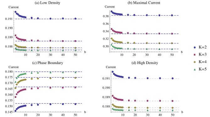
Figure 7: Plots for the TASEP on a tree of current versus b for $K=2,3,4,5$ using the simulation results. The dashed lines are the mean field theory results for the relevant values of K. Details of the plots are; (a) is in the low density phase with $\alpha=0.25$ and $\beta=1.0$. (b) is in the maximal current phase with $\alpha=1.0$ and $\beta=1.0$. (c) is on the phase boundary between low density and high density phases with $\alpha=0.25$ and $\beta=0.25$. (d) is in the high density phase with $\alpha=1.0$ and $\beta=0.25$.

In figure 8 we show the relationship between $k$, the level in the tree, and the average density of sites at that level for each of the four points on the phase diagram. Simulation results are shown for $b=2$ and $b=3$. These are compared against the exact results for the $b=1$ exact solution and the $b\rightarrow\infty$ mean field solution.

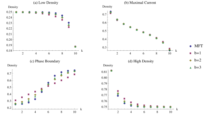
Figure 8: Density profiles for TASEP on a tree for $K=10$. The $b=2$ points are from simulation. These are compared with the $b=1$ results from the exact solution of the one-dimensional TASEP and the mean field theory which is exact in the limit $b\rightarrow\infty$. Details of the plots are: (a) is in the low density phase with $\alpha=0.25$ and $\beta=1.0$; (b) is in the maximal current phase with $\alpha=1.0$ and $\beta=1.0$; (c) is on the phase boundary between low density and high density phases with $\alpha=0.25$ and $\beta=0.25$; (d) is in the high density phase with $\alpha=1.0$ and $\beta=0.25$.

In figure 9 we show the relationship between current and $K$ for $b=2$ at the four points on the phase diagram. In each case these are compared with the corresponding mean field result and with the exact results for one dimension which is equivalent to $b=1$. In every case we find that the $b=2$ current lies between the MFT and $b=1$ current and that all three converge towards the same value for large $K$.

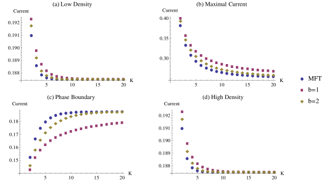
Figure 9: Plots for the TASEP on a tree of current versus K for $b=1$ using the exact 1D results, $b=2$ from the simulation results and for mean field theory. Details of the plots are; (a) is in the low density phase with $\alpha=0.25$ and $\beta=1.0$. (b) is in the maximal current phase with $\alpha=1.0$ and $\beta=1.0$. (c) is on the phase boundary between low density and high density phases with $\alpha=0.25$ and $\beta=0.25$. (d) is in the high density phase with $\alpha=1.0$ and $\beta=0.25$.

In summary, the simulations demonstrate that values of $b$ greater than one interpolate between the behaviour of the one-dimensional model and MFT. The convergence towards mean field behaviour is rapid with even $b=2$ being closer to mean field than to the $b=1$ behaviour in most cases. We have looked at estimating critical exponents for finite size behaviour and found the results inconclusive because of the relatively small values of K of the systems simulated.

7 Conclusion

In this paper we have investigated a generalisation of the one-dimensional TASEP to a tree lattice where the aggregate hopping rate from level to level remains constant. We have shown with this choice for hopping rates the TASEP on a tree shows a similar rich behaviour to the one-dimensional case. The mean field theory for the tree models is identical to the one-dimensional and predicts the correct phase diagram (which we confirm by simulation). We have shown that mean field theory becomes exact in the limiting case of large branching ratio or coordination number.

We have presented an exact solution for the two level tree ($K=2$) that allows the computation of any correlation function. Evaluating the integral representation of the solution by the saddle point method confirms the validity of MFT for an $n$-point correlation function when $n\ll b$ and we take $b\rightarrow\infty$. We also computed the steady-state current as a function of branching ratio $b$. The form of the solution is fairly complex for $K=2$ and we were not able to generalise it to higher values of $K$.

Our simulation results indicate that the convergence to the large branching ratio limit is quite rapid. We hope that the large branching ratio limit will be useful in a broader set of situations than we have dealt with here and we hope it may prove a useful limit for exploring more complex aspects of the TASEP, such as disorder, which are not tractable in the one-dimensional case.

With regard to applications of the model, it has the appealing characteristic that the “total hopping capacity” is the same at each level of the tree. Any natural process that generates a tree like distribution network by successively dividing capacity will approximate this characteristic. As mentioned in the introduction the optimal design of these systems has been the main focus of research in this area. However, the model we analyse here attempts to answer a different question; what steady-state current is achieved for specific values of the source input rate, transport rate in the distribution network and sink output rate. Our results show that the steady-state current has a non-trivial dependence on these parameters. Interestingly, we provide a full analytic solution for the two level tree (or star network or explosion network) that is one of the simplest optimal networks. It remains an open question as to which application areas are best addressed using a TASEP type model with our model for the hopping rates, but vehicular traffic is a reasonable candidate. Where it is applicable it predicts that the system can potentially experience a high density, low density or maximal current phase depending on how the parameters $\alpha,\beta$ position the system on the phase diagram Figure 2.

As a next step it would be nice to develop an approximation for the general tree that provides corrections to mean field theory and introduces $b$ dependence. It would also be valuable to look at other non-equilibrium processes on the tree.

Appendix A Equations for time evolution of a general correlation function for the TASEP on a general lattice

We can derive a very general result for the TASEP correlation functions on a arbitrary network using the master equation. In this appendix we use the master equation to derive an equation for the time evolution of the correlation function $c_{S}\left(t\right)$ defined in equation (19) and we show that the time evolution of $c_{S}\left(t\right)$ depends only the boundary sites of $S$ and their nearest neighbours outside of $S$.

Taking the time derivative of $c_{S}$$\left(t\right)$ and substituting for the time derivative of $P\left(\mathcal{C},t\right)$ using the master equation (11) gives

$$\frac{\partial c_{S}\left(t\right)}{\partial t}=\sum_{\mathcal{C^{\prime}}}P\left(\mathcal{C^{\prime}},t\right)\sum_{\mathcal{C}}W\left(\mathcal{C^{\prime}},\mathcal{C}\right)\left\{\left(\prod_{i\in S}\tau_{i}\right)-\left(\prod_{i\in S}\tau_{i}^{\prime}\right)\right\}.$$ (67)

The term in curly brackets has the effect of restricting the sums on $\mathcal{C}$ and $\mathcal{C^{\prime}}$ to configurations where all $\tau$ in $S$ are one or all $\tau^{\prime}$ in $S$ are one but not both.

We now focus on a TASEP on a general directed graph where particles can hop from site $i$ to site $j$ if there is a link from $i$ to $j$ and we specify the hopping rate as $h_{ij}$. In addition we identify a subset of “entry” sites where particles are introduced at a site dependent rate $\alpha_{i}$ and a subset of “exit” sites where particles are removed at rate $\beta_{j}$. This gives a transition matrix

$$W\left(\mathcal{C^{\prime}},\mathcal{C}\right)=\begin{cases}\alpha_{i}&\text{if }\mathcal{C^{\prime}},\mathcal{\,C}\>\text{are identical except at one entry site where }\tau_{i}^{\prime}=0,\tau_{i}=1,\\ h_{ij}&\text{if }\mathcal{C^{\prime}},\mathcal{\,C}\>\text{are identical except at two connected sites where }\tau_{i}^{\prime}=1,\tau_{i}=0,\tau_{j}^{\prime}=0,\tau_{j}=1,\\ \beta_{i}&\text{if }\mathcal{C^{\prime}},\mathcal{\,C}\>\text{are identical except at one exit site where }\tau_{i}^{\prime}=1,\tau_{i}=0,\\ 0&\mathrm{otherwise.}\end{cases}$$

We can express this transition matrix as;

$$W\left(\mathcal{C^{\prime}},\mathcal{C}\right) = \sum_{i\in S_{entry}^{all}}\alpha_{i}\left(1-\tau_{i}^{\prime}\right)\tau_{i}\prod_{j\in S^{all}\left[\overline{i}\right]}\delta\left[\tau_{j}^{\prime}=\tau_{j}\right]$$

$$+ \sum_{\left(i,j\right)\in E}h_{ij}\tau_{i}^{\prime}\left(1-\tau_{i}\right)\left(1-\tau_{j}^{\prime}\right)\tau_{j}\prod_{k\in S^{all}\left[\overline{i},\overline{j}\right]}\delta\left[\tau_{k}^{\prime}=\tau_{k}\right]$$

$$+ \sum_{i\in S_{exit}^{all}}\beta_{i}\tau_{i}^{\prime}\left(1-\tau_{i}\right)\prod_{j\in S^{all}\left[\overline{i}\right]}\delta\left[\tau_{j}^{\prime}=\tau_{j}\right]$$

where the $\delta[\textrm{statement}]$ is a generalised Kronecker delta; equal to unity if statement is true and zero otherwise. $E$ is the set of all directed edges,$S^{all}$ is the set of all sites in the lattice and the subsets are defined as

$$S_{entry}^{all} =$$ subset of all entry sites,

$$S_{exit}^{all} =$$ subset of all exit sites

$$S^{all}\left[\overline{i},\overline{j},\ldots\right] = \text{subset of all sites excluding sites }i,j,\ldots$$

If we substitute this expression for $W\left(\mathcal{C^{\prime}},\mathcal{C}\right)$ into equation (67) it has the effect of picking out terms at the boundary of $S.$ Some algebra gives the general result

$$\frac{\partial c\left(S,t\right)}{\partial t} = \sum_{i\in S_{entry}}\alpha_{i}\left\{c\left(S\left[\overline{i}\right],t\right)-c\left(S,t\right)\right\}$$ (68)

$$+ \sum_{j\in S_{in}}\sum_{i\in I\left(j\right)}h_{ij}\left\{c\left(S\left[i,\overline{j}\right],t\right)-c\left(S\left[i\right],t\right)\right\}$$

$$- \sum_{i\in S_{out}}\sum_{j\in O\left(i\right)}h_{ij}\left\{c\left(S,t\right)-c\left(S\left[j\right],t\right)\right\}$$

$$- \sum_{i\in S_{exit}}\beta_{i}c\left(S,t\right)$$

Where $S\left[\overline{i}\right]$ is the subset of sites obtained by subtracting the site $i$ from $S$, $S\left[i\right]$ is obtained by adding site $i$ to $S$ and $S\left[i,\overline{j}\right]$is obtained by adding site $i$ and subtracting site $j$. The subsets used for the sums in equation (68) are defined in table (1).

The physical meaning of equation (68) is clear if we take $S$ to contain a single bulk site; it is then a simple statement of conservation of particles. We can extend this to arbitrary $S$ by dividing all possible configurations into two sets; those with all sites in $S$ occupied and those with at least one vacant. The equation can then be obtained by considering the rate of transitions between the two sets.

Appendix B Inductive proof that MFT is exact on the line $\alpha+\beta=1$

In this appendix we will prove that any set of sites $S$ will satisfy equation (24) which we reproduce here for convenience

$$0 = \delta\left[\left(1,1\right)\in S\right]+\sum_{\left(i,j\right)\in S_{in}}\frac{1}{b^{i-1}}-\sum_{\left(i,j\right)\in S_{out}}\frac{1}{b^{i}}\sum_{(i+1,k)\in O\left(i,j\right)}1-\sum_{i\in S_{exit}}1.$$ (69)

If $S$ is the empty set then equation (69) is clearly satisfied as all terms on the right hand side are zero. If we now assume that it is true for an arbitrary $S$ then we need to prove that it also holds for any $S^{\prime}$ constructed by adding any single site to $S$. We can then assert the inductive step starting with the empty set and adding sites to obtain any possible collection of sites. When adding sites we need to consider eight possible scenarios which modify the subsets of $S$ ($S_{in}$,$S_{out}$, $\left\{\left(1,1\right)\right\}$, $S_{exit}$) that appear in equation (69) in different ways.

1. Add a site at $\left(1,1\right)$ that is disconnected from any site in $S$.

2. Add a site at $\left(1,1\right)$ that is connected to $m$ sites in $S$ at level 2.

3. Add an exit site $\left(K,i\right)$ that is disconnected from any site in $S$.

4. Add an exit site $\left(K,i\right)$ that is connected to $m$ sites in $S$ at level $K-1$.

5. Add a bulk site $\left(k,i\right)$ that is disconnected from any site in $S$.

6. Add a bulk site $\left(k,i\right)$ that is connected to $m$ sites in $S$ at level $k+1$ but no sites at level $k-1$.

7. Add a bulk site $\left(k,i\right)$ that is connected to one site in $S$ at level $k-1$ but no sites at level $k+1$.

8. Add a bulk site $\left(k,i\right)$ that is connected to one site in $S$ at level $k-1$ and $m$ sites at level $k+1$.

Scenario	First term	Second term	Third term	Fourth term	Total
1	$+1$	$0$	$-1$	$0$	$0$
2	$+1$	$-\frac{m}{b}$	$-\frac{b-m}{b}$	$0$	$0$
3	$0$	$+\frac{1}{b^{K-1}}$	$0$	$-\frac{1}{b^{K-1}}$	$0$
4	$0$	$0$	$+\frac{1}{b^{K-1}}$	$-\frac{1}{b^{K-1}}$	$0$
5	$0$	$+\frac{1}{b^{k-1}}$	$-\frac{1}{b^{k-1}}$	$0$	$0$
6	$0$	$+\frac{1}{b^{k-1}}-\frac{m}{b^{k}}$	$-\frac{b-m}{b^{k}}$	$0$	$0$
7	$0$	$0$	$+\frac{1}{b^{k-1}}-\frac{b}{b^{k}}$	$0$	$0$
8	$0$	$-\frac{m}{b^{k}}$	$+\frac{1}{b^{k-1}}-\frac{b-m}{b^{k}}$	$0$	$0$

Table 2: The change in each term on the right hand side of equation (69) from adding a single site to $S$ using each of the possible scenarios described in the text.

In table 2 we evaluate the impact of each scenario on the right hand side of equation (69). As we see the total change in the right hand side is zero in each scenario, so that we have proven that if $S$ satisfies equation (69) then so does $S^{{}^{\prime}}$. Therefore, starting with the empty set we can construct any possible set of sites and by induction it will also satisfy (69).

References

- [1] R A Blythe and M R Evans. Nonequilibrium steady states of matrix-product form: a solver’s guide. Journal of Physics A: Mathematical and Theoretical, 40:R333–R441, November 2007.
- [2] T Chou, K Mallick, and R K P Zia. Non-equilibrium statistical mechanics: from a paradigmatic model to biological transport. Reports on Progress in Physics, 74:116601, November 2011.
- [3] J Krug. Boundary-induced phase transitions in driven diffusive systems. Physical Review Letters, 67(14):1882–1885, September 1991.
- [4] B Derrida, E Domany, and D Mukamel. An exact solution of a one-dimensional asymmetric exclusion model with open boundaries. Journal of statistical physics, 69(3):667–687, 1992.
- [5] B Derrida, M R Evans, V Hakim, and V Pasquier. Exact solution of a 1D asymmetric exclusion model using a matrix formulation. Journal of Physics A: Mathematical and General, 26(7):1493–1517, April 1993.
- [6] G Schutz and E Domany. Phase transitions in an exactly soluble one-dimensional exclusion process. Journal of statistical physics, 72(1-2):277–296, 1993.
- [7] J de Gier and F H L Essler. Bethe ansatz solution of the asymmetric exclusion process with open boundaries. Physical review letters, 95(24):240601, 2005.
- [8] A Proeme, R A Blythe, and M R Evans. Dynamical transition in the open-boundary totally asymmetric exclusion process. Journal of Physics A: Mathematical and Theoretical, 44(3):035003, January 2011.
- [9] T Sasamoto. One-dimensional partially asymmetric simple exclusion process with open boundaries: orthogonal polynomials approach. Journal of Physics A: Mathematical and General, 32(41):7109, October 1999.
- [10] R A Blythe, M R Evans, F Colaiori, and F H L Essler. Exact solution of a partially asymmetric exclusion model using a deformed oscillator algebra. Journal of Physics A: Mathematical and General, 33(12):2313, March 2000.
- [11] B Derrida, J L Lebowitz, and E R Speer. Exact large deviation functional of a stationary open driven diffusive system: the asymmetric exclusion process. Journal of statistical physics, 110(3-6):775–810, 2003.
- [12] B Derrida, S A Janowsky, J L Lebowitz, and E R Speer. Exact solution of the totally asymmetric simple exclusion process: Shock profiles. Journal of Statistical Physics, 73(5-6):813–842, December 1993.
- [13] M R Evans, P A Ferrari, and K Mallick. Matrix representation of the stationary measure for the multispecies TASEP. Journal of Statistical Physics, 135(2):217–239, 2009.
- [14] A Lazarescu and K Mallick. An exact formula for the statistics of the current in the TASEP with open boundaries. Journal of Physics A: Mathematical and Theoretical, 44(31):315001, August 2011.
- [15] M R Evans, Y Kafri, K E P Sugden, and J Tailleur. Phase diagrams of two-lane driven diffusive systems. Journal of Statistical Mechanics: Theory and Experiment, 2011(06):P06009, 2011.
- [16] I Neri, N Kern, and Andrea Parmeggiani. Totally asymmetric simple exclusion process on networks. Physical Review Letters, 107(6):068702, 2011.
- [17] I Neri, N Kern, and A. Parmeggiani. Modelling cytoskeletal traffic: an interplay between passive diffusion and active transport. arXiv:1212.0437, December 2012.
- [18] M Basu and P K Mohanty. Asymmetric simple exclusion process on a cayley tree. Journal of Statistical Mechanics: Theory and Experiment, 2010(10):P10014, October 2010.
- [19] Jayanth R. Banavar, Melanie E. Moses, James H. Brown, John Damuth, Andrea Rinaldo, Richard M. Sibly, and Amos Maritan. A general basis for quarter-power scaling in animals. Proceedings of the National Academy of Sciences, 107(36):15816–15820, September 2010. PMID: 20724663.
- [20] Peter Sheridan Dodds. Optimal form of branching supply and collection networks. Physical review letters, 104(4):048702, 2010.
- [21] Michael T. Gastner and Mark EJ Newman. The spatial structure of networks. The European Physical Journal B-Condensed Matter and Complex Systems, 49(2):247–252, 2006.
- [22] D T Gillespie. Exact stochastic simulation of coupled chemical reactions. The Journal of Physical Chemistry, 81(25):2340–2361, December 1977.