On the Cauchy problem for a new integrable two-component system with peakon and weak kink solutions

Abstract

This paper is contributed to study the Cauchy problem of a new integrable two-component system with peaked soliton (peakon) and weak kink solutions. We first establish the local well-posedness result for the Cauchy problem in Besov spaces, and then present a precise blow-up scenario and a new blow-up result for strong solutions to the system.

2010 Mathematics Subject Classification: 35G25, 35L05

Keywords: Two-component system, peakon, weak kink solutions, Cauchy problem, local well-posedness, Besov spaces, blow-up.

1 Introduction

In the past two decades, a large amount of literature was devoted to the celebrated Camassa-Holm (CH) equation [4]

$$m_{t}+um_{x}+2u_{x}m+bu_{x}=0,\quad m=u-u_{xx},$$

where $b$ is an arbitrary constant, which models the unidirectional propagation of shallow water waves over a flat bottom. Here $u(t,x)$ stands for the fluid velocity at time $t$ in the spatial $x$ direction [4, 24, 42]. CH is also a model for the propagation of axially symmetric waves in hyperelastic rods [20]. It has a bi-Hamiltonian structure and is completely integrable [4, 31]. Also there is a geometric interpretation of CH in terms of geodesic flow on the diffeomorphism group of the circle [16]. Its solitary waves are peaked [5, 49]. They are orbitally stable and interact like solitons [2, 19]. It is also worth pointing out the peaked solitary waves replicate a feature that is characteristic for the waves of great height-waves of largest amplitude that are exact solutions of the governing equations for water waves, cf. the discussion in the papers [9, 13].

The Cauchy problem and initial boundary value problem for CH have been studied extensively [10, 11, 21, 29]. It has been shown that this equation is locally well-posed [10, 11, 21] for initial data $u_{0}\in H^{s}(\mathbb{R})$, $s>\frac{3}{2}$. Moreover, it has global strong solutions [8, 10, 11] and also finite time blow-up solutions [8, 10, 11, 12]. On the other hand, it has global weak solutions in $H^{1}(\mathbb{R})$ [3, 18, 57]. The advantage of CH in comparison with the KdV equation lies in the fact that CH has peaked solitons and models wave breaking [5, 12] (by wave breaking we understand that the wave remains bounded while its slope becomes unbounded in finite time [54]).

Another important integrable equation admitting peaked soliton (peakon) is the famous Degasperis-Procesi (DP) equation [23]

$$m_{t}+um_{x}+3u_{x}m=0,\quad m=u-u_{xx},$$

which is regarded as a model for nonlinear shallow water dynamics [15, 17]. It was proved in [22] that the DP equation has a bi-Hamiltonian structure and an infinite number of conservation laws, and admits exact peakon solutions which are analogous to the CH peakons. The Cauchy problem and initial boundary value problem for DP have been studied extensively in [7, 27, 28, 29, 44, 62, 63]. Although DP is very similar to CH in many aspects, especially in the structure of equation, there are some essential differences between the two equations. One of the famous features of DP equation is that it has not only (periodic) peakon solutions [22, 63], but also (periodic) shock peakons [28, 45]. Besides, CH is a re-expression of geodesic flow on the diffeomorphism group [16], while the DP equation can be regarded as a non-metric Euler equation [25].

Note that the nonlinear terms in the CH and DP equations are both quadratic. Indeed, there exist integrable systems admitting peakons and nonlinear cubic terms, which are the modified CH equation

$$m_{t}+((u^{2}-u^{2}_{x})m)_{x}+bu_{x}=0,\quad m=u-u_{xx}$$ (1.1)

with a constant $b$, and the Novikov equation

$$m_{t}+u^{2}m_{x}+3uu_{x}m=0,\quad m=u-u_{xx}.$$

Eq.(1.1) was proposed independently in [31, 32, 47, 50]. The Lax pair and cusped soliton (cuspon) solutions for Eq.(1.1) have been studied in [50, 51]. Recently, the formation of singularities for Eq.(1.1), a wave-breaking mechanism and the peakon stability of Eq.(1.1) in the case of $b=0$ were investigated in [38]. The Novikov equation was proposed in [46] and its Lax pair, bi-Hamiltonian structure, peakon solutions, well-posedness, blow-up phenomena and global weak solutions have been studied extensively in [39, 41, 46, 55]. Very recently, the following integrable equation with both quadratic and cubic nonlinearity

$$m_{t}+\frac{1}{2}k_{1}((u^{2}-u^{2}_{x})m)_{x}+\frac{1}{2}k_{2}(um_{x}+2u_{x}m)+bu_{x}=0,$$ (1.2)

was investigated, where $m=u-u_{xx}$, $b$, $k_{1}$, and $k_{2}$ are three arbitrary constants. Eq.(1.2) was first proposed by Fokas in [30]. Its Lax pair, bi-Hamiltonian structure, peakons, weak kinks, kink-peakon interactional, and smooth soliton solutions were studied recently in [52].

A natural idea is to extend such study to the multi-component generalized systems. One of the most popular is the following integrable two-component Camassa-Holm shallow water system (2CH) [6, 14]:

$$\left\{\begin{array}[]{ll}m_{t}+um_{x}+2u_{x}m+\sigma\rho\rho_{x}=0,\\ \rho_{t}+(u\rho)_{x}=0,\end{array}\right.$$

where $m=u-u_{xx}$ and $\sigma=\pm 1$, which becomes CH equation when $\rho\equiv 0$. The Cauchy problems of (2CH) with $\sigma=-1$ and with $\sigma=1$ have been studied in [26] and [14, 33, 35, 37], respectively. Local well-posedness for (2CH) with the initial data in Sobolev spaces and in Besov spaces have been established in [14, 27, 37]. The blow-up phenomena and global existence of strong solutions to (2CH) in Sobolev spaces have been derived in [27, 33, 37]. The analyticity of solutions to the Cauchy problem for (2CH) and the initial boundary value problem for (2CH) have been studied in [58] and [61], respectively. Recently, the existence of global weak solutions for (2CH) with $\sigma=1$ has been investigated in [35]. Another two famous systems are the modified two-component Camassa-Holm system (M2CH) [40]:

$$\left\{\begin{array}[]{ll}m_{t}+um_{x}+2u_{x}m+\sigma\rho\bar{\rho}_{x}=0,\\ \rho_{t}+(u\rho)_{x}=0,\end{array}\right.$$

with $m=u-u_{xx}$, $\rho=(1-\partial^{2}_{x})(\bar{\rho}-\bar{\rho}_{0})$, $\sigma=\pm 1$, and the two-component Degasperis-Procesi system (2DP) [48]:

$$\left\{\begin{array}[]{ll}m_{t}+um_{x}+3u_{x}m+b\rho\rho_{x}=0,\\ \rho_{t}+u\rho_{x}+2u_{x}\rho=0,\end{array}\right.$$

with $m=u-u_{xx}$ and a real constant $b$. When $\rho\equiv 0$, (M2CH) and (2DP) are reduced to CH and DP equations, respectively. The Cauchy problems and initial boundary value problems for (M2CH) and (2DP) have been studied in many works, for example [34, 36, 53, 60, 61] and [59, 61], respectively. It is noted to point out that the nonlinear terms in above three two-component systems are all quadratic.

In this paper, we consider the following integrable two-component system with both quadratic and cubic nonlinearity proposed in [56]:

$$\left\{\begin{array}[]{ll}m_{t}+\frac{1}{2}[(uv-u_{x}v_{x})m]_{x}-\frac{1}{2}(uv_{x}-u_{x}v)m+bu_{x}=0,\\ n_{t}+\frac{1}{2}[(uv-u_{x}v_{x})n]_{x}+\frac{1}{2}(uv_{x}-u_{x}v)n+bv_{x}=0,\end{array}\right.$$ (1.3)

where $m=u-u_{xx}$, $n=v-v_{xx}$, and $b$ takes an arbitrary value. System (1.3) is reduced to the CH equation, the modified cubic CH equation Eq.(1.1), and the generalized CH equation Eq.(1.2) as $v=2$, $v=2u$, and $v=k_{1}u+k_{2}$, respectively. Integrability of this system, its bi-Hamiltonian structure, and infinitely many conservation laws were already presented in [56]. In addition, this system is the first two-component system admitting weak kink solutions. Let us set up the Cauchy problem for the above system as follows:

$$\left\{\begin{array}[]{ll}m_{t}+\frac{1}{2}(uv-u_{x}v_{x})m_{x}=-\frac{1}{2}(u_{x}n+v_{x}m)m+\frac{1}{2}(uv_{x}-u_{x}v)m-bu_{x},\\ n_{t}+\frac{1}{2}(uv-u_{x}v_{x})n_{x}=-\frac{1}{2}(u_{x}n+v_{x}m)n-\frac{1}{2}(uv_{x}-u_{x}v)n-bv_{x},\\ m(0,x)=m_{0}(x),\\ n(0,x)=n_{0}(x).\end{array}\right.$$ (1.4)

By using the same approach in [58], the analytic solutions to System (1.4) can be readily proved in both variables, globally in space and locally in time. However, the goal of this paper is to establish the local well-posedness regime for the Cauchy problem in Besov spaces, present the precise blow-up scenario and a new blow-up result for strong solutions to the system, and derive the peakon and weak kink solutions.

With regard to the locally well-posed problem, we first apply the classical Kato semigroup theory to obtain the local well-posedness for System (1.4) with initial data $(m_{0},n_{0})$ belonging in Sobolev space $H^{s}(\mathbb{R})\times H^{s}(\mathbb{R})$ as $s\geq 1$. Subsequently, we take advantage of the transport equation theory, Littlewood-Paley’s decomposition and some fine estimates of Besov spaces to establish the local well-posedness for System (1.4) in Besov spaces (see Theorem 3.2 below), which particularly implies the system is locally well-posed with initial data $(m_{0},n_{0})\in H^{s}(\mathbb{R})\times H^{s}(\mathbb{R})$ for $\frac{1}{2}<s\neq\frac{3}{2}$. This almost improves the corresponding result by using Kato’s semigroup approach.

In order to investigate the blow-up phenomena, we here make good use of the fine structure of System (1.4). It is not difficult to verify that System (1.4) possesses the following two conservation laws:

$$H_{1}=\frac{1}{2}\int_{\mathbb{R}}(uv+u_{x}v_{x})dx=\frac{1}{2}\int_{\mathbb{R}}undx=\frac{1}{2}\int_{\mathbb{R}}vmdx,$$

$$H_{2}=\frac{1}{4}\int_{\mathbb{R}}\left((u^{2}v_{x}+u^{2}_{x}v_{x}-2uu_{x}v)n+2b(uv_{x}-u_{x}v)\right)dx.$$

Indeed, as mentioned before, this system has infinitely many conservation laws. But, unfortunately, one cannot seem to seek and then utilize some of them to control the quantities $||u(t,\cdot)||_{L^{\infty}}$ and $||v(t,\cdot)||_{L^{\infty}}$ directly. While it is very important to bound them in studying the blow-up phenomena of System (1.4). This difficulty has been overcome in some sense by exploiting the characteristic ODE related to System (1.4) to establish some invariant properties of the solutions and making good use of the structure of the system itself (we here need to treat two cross terms $\frac{1}{2}(uv_{x}-u_{x}v)m$ and $-\frac{1}{2}(uv_{x}-u_{x}v)n$ in the system), see Lemma 4.2 below. It is noted to point out that, for the special case Eq.(1.1) as $b=0$, with the conserved quantity $\int_{\mathbb{R}}umdx=||u||^{2}_{H^{1}(\mathbb{R})}$ in hand, one can directly control $||u(t,\cdot)||_{L^{\infty}}$ by using Sobolev’s embedding theorem, that is, $||u(t,\cdot)||_{L^{\infty}(\mathbb{R})}\leq C||u(t,\cdot)||_{H^{1}(\mathbb{R})}=C||u_{0}(\cdot)||_{H^{1}(\mathbb{R})}$, for all $t\in[0,T)$. And thus the blow-up phenomena of Eq.(1.1) with $b=0$ has been studied in [38]. On the other hand, in view of the uselessness of the conservation laws of System (1.4) again (mainly because the regularity is not high enough), we directly investigate the transport equation in terms of the flow $\frac{1}{2}(u_{x}n+v_{x}m)$ which is the slope of $\frac{1}{2}(uv-u_{x}v_{x})$ (see Lemma 4.3 below) to derive a new blow-up result with respect to initial data (see Theorem 4.3 below). Overall, we haven’t used any conservation laws rather than the almost symmetrical structure of System (1.4) in the whole paper.

The rest of our paper is organized as follows. In Section 2, we will recall some facts on the Littlewood-Paley decomposition, the nonhomogeneous Besov spaces and their some useful properties, and the transport equation theory as well. In Section 3, we establish the local well-posedness of System (1.4). In Section 4, we derive the precise blow-up scenario and a new blow-up result of strong solutions to System (1.4). Section 5 is devoted to discussing peakon and weak kink solutions.

2 Preliminaries

In this section, we will recall some facts on the Littlewood-Paley decomposition, the nonhomogeneous Besov spaces and their some useful properties, and the transport equation theory, which will be used in the sequel.

Proposition 2.1.

[1] (Littlewood-Paley decomposition) There exists a couple of smooth functions $(\chi,\varphi)$ valued in $[0,1]$, such that $\chi$ is supported in the ball $B\triangleq\{\xi\in\mathbb{R}^{n}:|\xi|\leq\frac{4}{3}\}$, and $\varphi$ is supported in the ring $C\triangleq\{\xi\in\mathbb{R}^{n}:\frac{3}{4}\leq|\xi|\leq\frac{8}{3}\}$. Moreover,

$$\forall\,\ \xi\in\mathbb{R}^{n},\,\ \chi(\xi)+{\sum\limits_{q\in\mathbb{N}}\varphi(2^{-q}\xi)}=1,$$

and

$$\textrm{supp}\,\ \varphi(2^{-q}\cdot)\cap\textrm{supp}\,\ \varphi(2^{-q^{\prime}}\cdot)=\emptyset,\,\ \text{if}\,\ |q-q^{\prime}|\geq 2,$$

$$\textrm{supp}\,\ \chi(\cdot)\cap\textrm{supp}\,\ \varphi(2^{-q}\cdot)=\emptyset,\,\ \text{if}\,\ q\geq 1.$$

Then for all $u\in\mathcal{S^{\prime}}$, we can define the nonhomogeneous dyadic blocks as follows. Let

$$\Delta_{q}{u}\triangleq 0,\,\ if\,\ q\leq-2,$$

$$\Delta_{-1}{u}\triangleq\chi(D)u=\mathcal{F}^{-1}\chi\mathcal{F}u,$$

$$\Delta_{q}{u}\triangleq\varphi(2^{-q}D)u=\mathcal{F}^{-1}\varphi(2^{-q}\xi)\mathcal{F}u,\,\ if\,\ q\geq 0.$$

Hence,

$$u={\sum\limits_{q\in\mathbb{Z}}}\Delta_{q}{u}\quad in\,\ \mathcal{S^{\prime}}(\mathbb{R}^{n}),$$

where the right-hand side is called the nonhomogeneous Littlewood-Paley decomposition of $u$.

Remark 2.1.

(1) The low frequency cut-off $S_{q}$ is defined by

$$S_{q}{u}\triangleq{\sum\limits_{p=-1}^{q-1}}\Delta_{p}{u}=\chi(2^{-q}D)u=\mathcal{F}^{-1}\chi(2^{-q}\xi)\mathcal{F}u,\,\ \forall\,\ q\in\mathbb{N}.$$

(2) The Littlewood-Paley decomposition is quasi-orthogonal in $L^{2}$ in the following sense:

$$\Delta_{p}\Delta_{q}{u}\equiv 0,\quad\text{if}\,\ |p-q|\geq 2,$$

$$\Delta_{q}(S_{p-1}u\Delta_{p}{v})\equiv 0,\quad\text{if}\,\ |p-q|\geq 5,$$

for all $u,v\in\mathcal{S^{\prime}}(\mathbb{R}^{n})$.
(3) Thanks to Young’s inequality, we get

$$||\Delta_{q}{u}||_{L^{p}},\,\ ||S_{q}{u}||_{L^{p}}\leq C||u||_{L^{p}},\quad\forall\,\ 1\leq p\leq\infty,$$

where $C$ is a positive constant independent of $q$.

Definition 2.1.

[1] (Besov spaces) Let $s\in\mathbb{R},1\leq p,r\leq\infty$. The nonhomogeneous Besov space $B^{s}_{p,r}(\mathbb{R}^{n})$ ($B^{s}_{p,r}$ for short) is defined by

$$B^{s}_{p,r}(\mathbb{R}^{n})\triangleq\{f\in\mathcal{S^{\prime}}(\mathbb{R}^{n}):||f||_{B^{s}_{p,r}}<\infty\},$$

where

$$||f||_{B^{s}_{p,r}}\triangleq||2^{qs}\Delta_{q}{f}||_{l^{r}(L^{p})}=||(2^{qs}||\Delta_{q}{f}||_{L^{p}})_{q\geq-1}||_{l^{r}}.$$

If $s=\infty$, $B^{\infty}_{p,r}\triangleq\bigcap\limits_{s\in\mathbb{R}}B^{s}_{p,r}$.

Definition 2.2.

Let $T>0$, $s\in\mathbb{R}$ and $1\leq p\leq\infty$. Set

$$E^{s}_{p,r}(T)\triangleq C([0,T];B^{s}_{p,r})\cap C^{1}{([0,T];B^{s-1}_{p,r})},\quad\text{if}\,\ r<\infty,$$

$$E^{s}_{p,\infty}(T)\triangleq L^{\infty}([0,T];B^{s}_{p,\infty})\cap Lip\,([0,T];B^{s-1}_{p,\infty})$$

and

$$E^{s}_{p,r}\triangleq\bigcap\limits_{T>0}E^{s}_{p,r}(T).$$

Remark 2.2.

By Definition 2.1 and Remark 2.1(3), we can deduce that

$$||\Delta_{q}{u}||_{B^{s}_{p,r}},\,\ ||S_{q}{u}||_{B^{s}_{p,r}}\leq C||u||_{B^{s}_{p,r}},$$

where $C$ is a positive constant independent of $q$.

In the following proposition, we list some important properties of Besov spaces.

Proposition 2.2.

[1, 37] Suppose that $s\in\mathbb{R},1\leq p,r,p_{i},r_{i}\leq\infty,i=1,2.$ We have
(1) Topological properties: $B^{s}_{p,r}$ is a Banach space which is continuously embedded in $\mathcal{S^{\prime}}$.
(2) Density: $\mathcal{C}^{\infty}_{c}$ is dense in $B^{s}_{p,r}$ $\Longleftrightarrow 1\leq p,r<\infty.$
(3) Embedding: $B^{s}_{p_{1},r_{1}}\hookrightarrow B^{s-n({1\over p_{1}}-{1\over p_{2}})}_{p_{2},r_{2}}$,    if $p_{1}\leq p_{2}$ and $r_{1}\leq r_{2}$,

$$B^{s_{2}}_{p,r_{2}}\hookrightarrow B^{s_{1}}_{p,r_{1}}\quad\text{locally compact},\quad\text{if}\,\ \,s_{1}<s_{2}.$$

(4) Algebraic properties: $\forall s>0$, $B^{s}_{p,r}\bigcap L^{\infty}$ is an algebra. Moreover, $B^{s}_{p,r}$ is an algebra, provided that $s>{n\over p}$ or $s\geq{n\over p}\,\ and\,\ r=1$.
(5) 1-D Morse-type estimates:
(i) $\forall s_{1}\leq\frac{1}{p}<s_{2}$ ($s_{2}\geq{1\over p}$ if $r=1$) and $s_{1}+s_{2}>0$, we have

$$||fg||_{B^{s_{1}}_{p,r}(\mathbb{R})}\leq C||f||_{B^{s_{1}}_{p,r}(\mathbb{R})}||g||_{B^{s_{2}}_{p,r}(\mathbb{R})}.$$ (2.1)

(ii)For $s>0$,

$$||fg||_{B^{s}_{p,r}(\mathbb{R})}\leq C(||f||_{B^{s}_{p,r}(\mathbb{R})}||g||_{L^{\infty}(\mathbb{R})}+||g||_{B^{s}_{p,r}(\mathbb{R})}||f||_{L^{\infty}(\mathbb{R})}).$$ (2.2)

(iii) In Sobolev spaces $H^{s}(\mathbb{R})=B^{s}_{2,2}(\mathbb{R})$, we have for $s>0$,

$$||f\partial_{x}g||_{H^{s}(\mathbb{R})}\leq C(||f||_{H^{s+1}(\mathbb{R})}||g||_{L^{\infty}(\mathbb{R})}+||f||_{L^{\infty}(\mathbb{R})}||\partial_{x}g||_{H^{s}(\mathbb{R})}),$$ (2.3)

where $C$ is a positive constant independent of $f$ and $g$.
(6) Complex interpolation:

$$\quad\quad\quad||f||_{B^{\theta{s_{1}}+(1-\theta){s_{2}}}_{p,r}}\leq||f||^{\theta}_{B^{s_{1}}_{p,r}}||f||^{1-\theta}_{B^{s_{2}}_{p,r}},\quad\forall u\in B^{s_{1}}_{p,r}\cap B^{s_{1}}_{p,r},\quad\forall\theta\in[0,1].$$ (2.4)

(7) Fatou lemma: if $(u_{n})_{n\in\mathbb{N}}$ is bounded in $B^{s}_{p,r}$ and $u_{n}\to u$ in $\mathcal{S^{\prime}}$, then $u\in B^{s}_{p,r}$ and

$$||u||_{B^{s}_{p,r}}\leq\liminf\limits_{n\to\infty}||u_{n}||_{B^{s}_{p,r}}.$$

(8) Let $m\in\mathbb{R}$ and $f$ be an $S^{m}$-multiplier (i.e., $f:\mathbb{R}^{n}\to\mathbb{R}$ is smooth and satisfies that for all $\alpha\in\mathbb{N}^{n}$, there exists a constant $C_{\alpha}$ such that $|\partial^{\alpha}{f(\xi)}|\leq C_{\alpha}(1+|\xi|)^{m-|\alpha|}$ for all $\xi\in\mathbb{R}^{n}$). Then the operator $f(D)$ is continuous from $B^{s}_{p,r}$ to $B^{s-m}_{p,r}.$

Now we state some useful results in the transport equation theory, which are crucial to the proofs of our main theorems later.

Lemma 2.1.

[1] (A priori estimates in Besov spaces) Let $1\leq p,r\leq\infty$ and $s>-\min({1\over p},1-{1\over p}).$ Assume that $f_{0}\in B^{s}_{p,r}$, $F\in L^{1}(0,T;B^{s}_{p,r})$, and $\partial_{x}v$ belongs to $L^{1}(0,T;B^{s-1}_{p,r})$ if $s>1+{1\over p}$ or to $L^{1}(0,T;B^{1\over p}_{p,r}\cap L^{\infty})$ otherwise. If $f\in L^{\infty}(0,T;B^{s}_{p,r})\bigcap C([0,T];\mathcal{S^{\prime}})$ solves the following 1-D linear transport equation:

$$(T)\left\{\begin{array}[]{l}\partial_{t}f+v\,\partial_{x}f=F,\\ f|_{t=0}=f_{0},\end{array}\right.$$

then there exists a constant $C$ depending only on $s,p$ and $r$, and such that the following statements hold:
(1) If $r=1$ or $s\neq 1+{1\over p}$,

$$||f(t)||_{B^{s}_{p,r}}\leq||f_{0}||_{B^{s}_{p,r}}\,+\,\int_{0}^{t}||F(\tau)||_{B^{s}_{p,r}}d\tau\,+\,C\int_{0}^{t}V^{\prime}(\tau)||f(\tau)||_{B^{s}_{p,r}}d\tau$$

or hence,

$$||f(t)||_{B^{s}_{p,r}}\leq e^{CV(t)}(||f_{0}||_{B^{s}_{p,r}}\,+\,\int_{0}^{t}e^{-CV(\tau)}||F(\tau)||_{B^{s}_{p,r}}d\tau)$$

with $V(t)=\int_{0}^{t}||\partial_{x}v(\tau)||_{B^{1\over p}_{p,r}\cap L^{\infty}}d\tau$ if $s<1+{1\over p}$ and $V(t)=\int_{0}^{t}||\partial_{x}v(\tau)||_{B^{s-1}_{p,r}}d\tau$ else.
(2) If $v=f$, then for all $s>0$, (1) holds true with $V(t)=\int_{0}^{t}||\partial_{x}v(\tau)||_{L^{\infty}}d\tau$.
(3) If $r<\infty$, then $f\in C([0,T];B^{s}_{p,r})$. If $r=\infty$, then $f\in C([0,T];B^{s^{\prime}}_{p,1})$ for all $s^{\prime}<s$.

Lemma 2.2.

[37] (A priori estimate in Sobolev spaces) Let $0<\sigma<1$. Assume that $f_{0}\in H^{\sigma}$, $F\in L^{1}(0,T;H^{\sigma})$, and $v,\partial_{x}v\in L^{1}(0,T;L^{\infty})$. If $f\in L^{\infty}(0,T;H^{\sigma})\bigcap C([0,T];\mathcal{S^{\prime}})$ solves $(T)$, then $f\in C([0,T];H^{\sigma})$, and there exists a constant $C$ depending only on $\sigma$ such that the following statement holds:

$$||f(t)||_{H^{\sigma}}\leq||f_{0}||_{H^{\sigma}}\,+\,\ C\int_{0}^{t}||F(\tau)||_{H^{\sigma}}d\tau\,+\,C\int_{0}^{t}V^{\prime}(\tau)||f(\tau)||_{H^{\sigma}}d\tau$$

or hence,

$$||f(t)||_{H^{\sigma}}\leq e^{CV(t)}(||f_{0}||_{H^{\sigma}}\,+\,\int_{0}^{t}||F(\tau)||_{H^{\sigma}}d\tau)$$

with $V(t)=\int_{0}^{t}(||v(\tau)||_{L^{\infty}}+||\partial_{x}v(\tau)||_{L^{\infty}})d\tau$.

Lemma 2.3.

[1] (Existence and uniqueness) Let $p,r,s,f_{0}$ and $F$ be as in the statement of Lemma 2.1. Assume that $v\in L^{\rho}(0,T;B^{-M}_{\infty,\infty})$ for some $\rho>1$ and $M>0$, and $\partial_{x}v\in L^{1}(0,T;{B^{s-1}_{p,r}})$ if $s>1+{1\over p}$ or $s=1+{1\over p}$ and $r=1$, and $\partial_{x}v\in L^{1}(0,T;B^{1\over p}_{p,\infty}\cap L^{\infty})$ if $s<1+{1\over p}$. Then (T) has a unique solution $f\in L^{\infty}(0,T;B^{s}_{p,r})\bigcap\,\big{(}\bigcap\limits_{s^{\prime}<s}C([0,T];B^{s^{\prime}}_{p,1})\big{)}$ and the inequalities of Lemma 2.1 can hold true. Moreover, if $r<\infty$, then $f\in C([0,T];B^{s}_{p,r})$.

3 Local well-posedness

In this section, we will establish the local well-posedness for System (1.4). To begin with, we apply the classical Kato’s semigroup theory [43] to obtain the local well-posedness of System (1.4) in Sobolev spaces. More precisely, we have

Theorem 3.1.

Suppose that $(m_{0},n_{0})\in H^{s}(\mathbb{R})\times H^{s}(\mathbb{R})$ with $s\geq 1$. There exists a maximal existence time $T=T(||m_{0}||_{H^{s}(\mathbb{R})},||n_{0}||_{H^{s}(\mathbb{R})})>0$, and a unique solution $(m,n)$ to System (1.4) such that

$$(m,n)\in C([0,T);H^{s}(\mathbb{R})\times H^{s}(\mathbb{R}))\cap C^{1}([0,T);H^{s-1}(\mathbb{R})\times H^{s-1}(\mathbb{R})).$$

Moreover, the solution depends continuously on the initial data, that is, the mapping $(m_{0},n_{0})\mapsto(m,n):$

$$H^{s}(\mathbb{R})\!\times\!H^{s}(\mathbb{R})\!\rightarrow\!C([0,T);H^{s}(\mathbb{R})\!\times\!H^{s}(\mathbb{R}))\cap C^{1}([0,T);H^{s-1}(\mathbb{R})\!\times\!H^{s-1}(\mathbb{R}))$$

is continuous.

Proof.

By going along the similar line of the proof in [26], one can readily prove the theorem. For the sake of simplicity, we omit the details here. ∎

Now we pay attention to the case in the nonhomogeneous Besov spaces. Uniqueness and continuity with respect to the initial data in some sense can be obtained by the following a priori estimates.

Lemma 3.1.

Let $1\leq p,r\leq\infty$ and $s>\max(1-\frac{1}{p},\frac{1}{p},\frac{1}{2})$. Suppose that we are given $(m^{(i)},n^{(i)})\in L^{\infty}(0,T;B^{s}_{p,r}\times B^{s}_{p,r})\cap C([0,T];\mathcal{S^{\prime}}\times\mathcal{S^{\prime}})$ ($i=1,2$) two solutions of System (1.4) with the initial data $(m_{0}^{(i)},n_{0}^{(i)})\in B^{s}_{p,r}\times B^{s}_{p,r}$ ($i=1,2$) and let $u^{(12)}\triangleq u^{(2)}-u^{(1)}$, $v^{(12)}\triangleq v^{(2)}-v^{(1)}$, and then $m^{(12)}\triangleq m^{(2)}-m^{(1)}$, $n^{(12)}\triangleq n^{(2)}-n^{(1)}$. Then for all $t\in[0,T]$, we have
(1) if $s>\max(1-\frac{1}{p},\frac{1}{p},\frac{1}{2})$, but $s\neq 2+\frac{1}{p}$, then

$$||m^{(12)}(t)||_{B^{s-1}_{p,r}}+||n^{(12)}(t)||_{B^{s-1}_{p,r}}$$

$$\leq (||m^{(12)}_{0}||_{B^{s-1}_{p,r}}+||n^{(12)}_{0}||_{B^{s-1}_{p,r}})$$

$$\times e^{C\int_{0}^{t}(||m^{(1)}(\tau)||_{B^{s}_{p,r}}+||m^{(2)}(\tau)||_{B^{s}_{p,r}}+||n^{(1)}(\tau)||_{B^{s}_{p,r}}+||n^{(2)}(\tau)||_{B^{s}_{p,r}}+1)^{2}d\tau}$$

$$\triangleq L(s-1;t);$$

(2) if $s=2+\frac{1}{p}$, then

$$||m^{(12)}(t)||_{B^{s-1}_{p,r}}+||n^{(12)}(t)||_{B^{s-1}_{p,r}}$$

$$\leq CL^{\theta}(s-1;t)((||m^{(1)}(t)||_{B^{s}_{p,r}}+||m^{(2)}(t)||_{B^{s}_{p,r}})^{1-\theta}$$

$$+(||n^{(1)}(t)||_{B^{s}_{p,r}}+||n^{(2)}(t)||_{B^{s}_{p,r}})^{1-\theta}),$$

where $\theta\in(0,1)$.

Proof.

It is obvious that $(m^{(12)},n^{(12)})\in L^{\infty}(0,T;B^{s}_{p,r}\times B^{s}_{p,r})\cap C([0,T];\mathcal{S^{\prime}}\times\mathcal{S^{\prime}})$ solves the following Cauchy problem of the transport equations:

$$\left\{\begin{array}[]{ll}\partial_{t}m^{(12)}+\frac{1}{2}(u^{(1)}v^{(1)}-u_{x}^{(1)}v_{x}^{(1)})\partial_{x}m^{(12)}=F(t,x),\\ \partial_{t}n^{(12)}+\frac{1}{2}(u^{(1)}v^{(1)}-u_{x}^{(1)}v_{x}^{(1)})\partial_{x}n^{(12)}=G(t,x),\\ m^{(12)}|_{t=0}=m^{(12)}_{0}\triangleq m^{(2)}_{0}-m^{(1)}_{0},\\ n^{(12)}|_{t=0}=n^{(12)}_{0}\triangleq n^{(2)}_{0}-n^{(1)}_{0},\end{array}\right.$$ (3.2)

where $F(t,x)\triangleq\frac{1}{2}\big{(}(u^{(1)}-m^{(1)})v_{x}^{(1)}-(v^{(1)}+n^{(1)})u_{x}^{(1)}-v_{x}^{(2)}m^{(2)}\big{)}m^{(12)}-\frac{1}{2}u_{x}^{(2)}m^{(2)}n^{(12)}+\frac{1}{2}\big{(}v_{x}^{(1)}m_{x}^{(2)}-(v^{(1)}+n^{(1)})m^{(2)}-2b\big{)}u_{x}^{(12)}+\frac{1}{2}\big{(}u_{x}^{(2)}m_{x}^{(2)}-(m^{(1)}-u^{(2)})m^{(2)}\big{)}v_{x}^{(12)}+\frac{1}{2}\big{(}v_{x}^{(1)}m^{(2)}-v^{(1)}m_{x}^{(2)}\big{)}u^{(12)}-\frac{1}{2}(u^{(2)}m^{(2)})_{x}v^{(12)}$,   and
$G(t,x)\triangleq\frac{1}{2}\big{(}(v^{(1)}-n^{(1)})u_{x}^{(1)}-(u^{(1)}+m^{(1)})v_{x}^{(1)}-u_{x}^{(2)}n^{(2)}\big{)}n^{(12)}-\frac{1}{2}v_{x}^{(2)}n^{(2)}m^{(12)}+\frac{1}{2}\big{(}u_{x}^{(1)}n_{x}^{(2)}-(u^{(1)}+m^{(1)})n^{(2)}-2b\big{)}v_{x}^{(12)}+\frac{1}{2}\big{(}v_{x}^{(2)}n_{x}^{(2)}-(n^{(1)}-v^{(2)})n^{(2)}\big{)}u_{x}^{(12)}+\frac{1}{2}\big{(}u_{x}^{(1)}n^{(2)}-u^{(1)}n_{x}^{(2)}\big{)}v^{(12)}-\frac{1}{2}(v^{(2)}n^{(2)})_{x}u^{(12)}$.

Claim. For all $s>\max(\frac{1}{p},\frac{1}{2})$ and $t\in[0,T]$, we have

$$||F(t)||_{B^{s-1}_{p,r}},\,\ ||G(t)||_{B^{s-1}_{p,r}}$$

$$\leq C(||m^{(12)}(t)||_{B^{s-1}_{p,r}}+||n^{(12)}(t)||_{B^{s-1}_{p,r}})$$

$$\times(||m^{(1)}(t)||_{B^{s}_{p,r}}+||m^{(2)}(t)||_{B^{s}_{p,r}}+||n^{(1)}(t)||_{B^{s}_{p,r}}+||n^{(2)}(t)||_{B^{s}_{p,r}}+1)^{2},$$

where $C=C(s,p,r,b)$ is a positive constant.
Indeed, for $s>1+\frac{1}{p}$, $B^{s-1}_{p,r}$ is an algebra, by Proposition 2.2 (4), we have

$$||(u^{(1)}-m^{(1)})v_{x}^{(1)}m^{(12)}||_{B^{s-1}_{p,r}}\leq(||u^{(1)}||_{B^{s-1}_{p,r}}+||m^{(1)}||_{B^{s-1}_{p,r}})||v_{x}^{(1)}||_{B^{s-1}_{p,r}}||m^{(12)}||_{B^{s-1}_{p,r}}.$$

Note that $(1-\partial_{x}^{2})^{-1}\in Op(S^{-2})$. According to Proposition 2.2 (8), we obtain for all $s\in\mathbb{R}$ and $i=1,2,12$,

$$||u^{(i)}||_{B^{s+2}_{p,r}}\approxeq||m^{(i)}||_{B^{s}_{p,r}}\quad\text{and}\quad||v^{(i)}||_{B^{s+2}_{p,r}}\approxeq||n^{(i)}||_{B^{s}_{p,r}}.$$ (3.4)

Then

$$||(u^{(1)}-m^{(1)})v_{x}^{(1)}m^{(12)}||_{B^{s-1}_{p,r}}\leq C||m^{(1)}||_{B^{s}_{p,r}}||n^{(1)}||_{B^{s}_{p,r}}||m^{(12)}||_{B^{s-1}_{p,r}}.$$

Similarly,

$$||(v^{(1)}+n^{(1)})u_{x}^{(1)}m^{(12)}||_{B^{s-1}_{p,r}}+||v_{x}^{(2)}m^{(2)}m^{(12)}||_{B^{s-1}_{p,r}}$$

$$\leq C(||m^{(1)}||_{B^{s}_{p,r}}||n^{(1)}||_{B^{s}_{p,r}}+||m^{(2)}||_{B^{s}_{p,r}}||n^{(2)}||_{B^{s}_{p,r}})||m^{(12)}||_{B^{s-1}_{p,r}},$$

$$||u_{x}^{(2)}m^{(2)}n^{(12)}||_{B^{s-1}_{p,r}}+||(u^{(2)}m^{(2)})_{x}v^{(12)}||_{B^{s-1}_{p,r}}\leq C||m^{(2)}||^{2}_{B^{s}_{p,r}}||n^{(12)}||_{B^{s-1}_{p,r}},$$

$$||\big{(}v_{x}^{(1)}m_{x}^{(2)}-(v^{(1)}+n^{(1)})m^{(2)}-2b\big{)}u_{x}^{(12)}||_{B^{s-1}_{p,r}}+||\big{(}v_{x}^{(1)}m^{(2)}-v^{(1)}m_{x}^{(2)}\big{)}u^{(12)}||_{B^{s-1}_{p,r}}$$

$$\leq C(||m^{(2)}||_{B^{s}_{p,r}}||n^{(1)}||_{B^{s}_{p,r}}+1)||m^{(12)}||_{B^{s-1}_{p,r}},$$

and

$$||\big{(}u_{x}^{(2)}m_{x}^{(2)}-(m^{(1)}-u^{(2)})m^{(2)}\big{)}v_{x}^{(12)}||_{B^{s-1}_{p,r}}$$

$$\leq C(||m^{(1)}||_{B^{s}_{p,r}}+||m^{(2)}||_{B^{s}_{p,r}})||m^{(2)}||_{B^{s}_{p,r}}||n^{(12)}||_{B^{s-1}_{p,r}}.$$

Hence,

$$||F(t)||_{B^{s-1}_{p,r}} \leq C(||m^{(12)}(t)||_{B^{s-1}_{p,r}}+||n^{(12)}(t)||_{B^{s-1}_{p,r}})$$

$$\times (||m^{(1)}(t)||_{B^{s}_{p,r}}+||m^{(2)}(t)||_{B^{s}_{p,r}}+||n^{(1)}(t)||_{B^{s}_{p,r}}+||n^{(2)}(t)||_{B^{s}_{p,r}}+1)^{2},$$

if $s>1+\frac{1}{p}$.
We can treat $||G(t)||_{B^{s-1}_{p,r}}$ for $s>1+\frac{1}{p}$ in a similar way.

On the other hand, if $\max(\frac{1}{p},\frac{1}{2})<s\leq{1+\frac{1}{p}}$, $B^{s}_{p,r}$ is an algebra. According to (2.1) and (3.4), one infers that

$$||\big{(}(u^{(1)}-m^{(1)})v_{x}^{(1)}-(v^{(1)}+n^{(1)})u_{x}^{(1)}-v_{x}^{(2)}m^{(2)}\big{)}m^{(12)}||_{B^{s-1}_{p,r}}$$

$$\leq C(||(u^{(1)}-m^{(1)})v_{x}^{(1)}||_{B^{s}_{p,r}}+||(v^{(1)}+n^{(1)})u_{x}^{(1)}||_{B^{s}_{p,r}}+||v_{x}^{(2)}m^{(2)}||_{B^{s}_{p,r}})||m^{(12)}||_{B^{s-1}_{p,r}}$$

$$\leq C(||m^{(1)}||_{B^{s}_{p,r}}||n^{(1)}||_{B^{s}_{p,r}}+||m^{(2)}||_{B^{s}_{p,r}}||n^{(2)}||_{B^{s}_{p,r}})||m^{(12)}||_{B^{s-1}_{p,r}},$$

$$||u_{x}^{(2)}m^{(2)}n^{(12)}||_{B^{s-1}_{p,r}}\leq C||u_{x}^{(2)}m^{(2)}||_{B^{s}_{p,r}}||n^{(12)}||_{B^{s-1}_{p,r}}\leq C||m^{(2)}||^{2}_{B^{s}_{p,r}}||n^{(12)}||_{B^{s-1}_{p,r}},$$

$$||\big{(}v_{x}^{(1)}m_{x}^{(2)}-(v^{(1)}+n^{(1)})m^{(2)}-2b\big{)}u_{x}^{(12)}||_{B^{s-1}_{p,r}}$$

$$\leq C||v_{x}^{(1)}u_{x}^{(12)}||_{B^{s}_{p,r}}||m_{x}^{(2)}||_{B^{s-1}_{p,r}}+C(||(v^{(1)}+n^{(1)})m^{(2)}||_{B^{s}_{p,r}}+|b|)||u_{x}^{(12)}||_{B^{s-1}_{p,r}}$$

$$\leq C(||m^{(2)}||_{B^{s}_{p,r}}||n^{(1)}||_{B^{s}_{p,r}}+1)||u^{(12)}||_{B^{s+1}_{p,r}}$$

$$\leq C(||m^{(2)}||_{B^{s}_{p,r}}||n^{(1)}||_{B^{s}_{p,r}}+1)||m^{(12)}||_{B^{s-1}_{p,r}},$$

$$||\big{(}u_{x}^{(2)}m_{x}^{(2)}-(m^{(1)}-u^{(2)})m^{(2)}\big{)}v_{x}^{(12)}||_{B^{s-1}_{p,r}}$$

$$\leq C(||u_{x}^{(2)}v_{x}^{(12)}||_{B^{s}_{p,r}}||m_{x}^{(2)}||_{B^{s-1}_{p,r}}+||(m^{(1)}-u^{(2)})m^{(2)}||_{B^{s}_{p,r}}||v_{x}^{(12)}||_{B^{s-1}_{p,r}})$$

$$\leq C(||m^{(1)}||_{B^{s}_{p,r}}+||m^{(2)}||_{B^{s}_{p,r}})||m^{(2)}||_{B^{s}_{p,r}}||v^{(12)}||_{B^{s+1}_{p,r}}$$

$$\leq C(||m^{(1)}||_{B^{s}_{p,r}}+||m^{(2)}||_{B^{s}_{p,r}})||m^{(2)}||_{B^{s}_{p,r}}||n^{(12)}||_{B^{s-1}_{p,r}},$$

$$||\big{(}v_{x}^{(1)}m^{(2)}-v^{(1)}m_{x}^{(2)}\big{)}u^{(12)}||_{B^{s-1}_{p,r}}$$

$$\leq C(||v_{x}^{(1)}m^{(2)}||_{B^{s}_{p,r}}||u^{(12)}||_{B^{s-1}_{p,r}}+||v^{(1)}u^{(12)}||_{B^{s}_{p,r}}||m_{x}^{(2)}||_{B^{s-1}_{p,r}})$$

$$\leq C||m^{(2)}||_{B^{s}_{p,r}}||n^{(1)}||_{B^{s}_{p,r}}||m^{(12)}||_{B^{s-1}_{p,r}},$$

and

$$||(u^{(2)}m^{(2)})_{x}v^{(12)}||_{B^{s-1}_{p,r}}$$

$$\leq C(||u_{x}^{(2)}m^{(2)}||_{B^{s}_{p,r}}||v^{(12)}||_{B^{s-1}_{p,r}}+||u^{(2)}v^{(12)}||_{B^{s}_{p,r}}||m_{x}^{(2)}||_{B^{s-1}_{p,r}})$$

$$\leq C||m^{(2)}||^{2}_{B^{s}_{p,r}}||n^{(12)}||_{B^{s-1}_{p,r}}.$$

Thus,

$$||F(t)||_{B^{s-1}_{p,r}} \leq C(||m^{(12)}(t)||_{B^{s-1}_{p,r}}+||n^{(12)}(t)||_{B^{s-1}_{p,r}})$$

$$\times (||m^{(1)}(t)||_{B^{s}_{p,r}}+||m^{(2)}(t)||_{B^{s}_{p,r}}+||n^{(1)}(t)||_{B^{s}_{p,r}}+||n^{(2)}(t)||_{B^{s}_{p,r}}+1)^{2},$$

if $\max(\frac{1}{p},\frac{1}{2})<s\leq{1+\frac{1}{p}}$.
We can also treat $||G(t)||_{B^{s-1}_{p,r}}$ for $\max(\frac{1}{p},\frac{1}{2})<s\leq{1+\frac{1}{p}}$ in a similar way. Therefore, we prove our Claim (3.3).

Applying Lemma 2.1 (1) and the fact that

$$V(t) \triangleq ||\partial_{x}(u^{(1)}v^{(1)}-u_{x}^{(1)}v_{x}^{(1)})||_{B^{\frac{1}{p}}_{p,r}\cap L^{\infty}}+||\partial_{x}(u^{(1)}v^{(1)}-u_{x}^{(1)}v_{x}^{(1)})||_{B^{s-2}_{p,r}}$$

$$\leq C||\partial_{x}(u^{(1)}v^{(1)}-u_{x}^{(1)}v_{x}^{(1)})||_{B^{s}_{p,r}}$$

$$\leq C||u^{(1)}||_{B^{s+2}_{p,r}}||v^{(1)}||_{B^{s+2}_{p,r}}$$

$$\leq C||m^{(1)}||_{B^{s}_{p,r}}||n^{(1)}||_{B^{s}_{p,r}}$$

for $s>\max(1-\frac{1}{p},\frac{1}{p},\frac{1}{2})$, we can obtain, for case (1),

$$||m^{(12)}(t)||_{B^{s-1}_{p,r}}\leq||m^{(12)}_{0}||_{B^{s-1}_{p,r}}+\int_{0}^{t}||F(\tau)||_{B^{s-1}_{p,r}}d\tau+C\int_{0}^{t}V(\tau)||m^{(12)}(\tau)||_{B^{s-1}_{p,r}}d\tau$$

and

$$||n^{(12)}(t)||_{B^{s-1}_{p,r}}\leq||n^{(12)}_{0}||_{B^{s-1}_{p,r}}+\int_{0}^{t}||G(\tau)||_{B^{s-1}_{p,r}}d\tau+C\int_{0}^{t}V(\tau)||n^{(12)}(\tau)||_{B^{s-1}_{p,r}}d\tau$$

which together with (3.3) yields

$$||m^{(12)}(t)||_{B^{s-1}_{p,r}}+||n^{(12)}(t)||_{B^{s-1}_{p,r}}$$

$$\leq ||m^{(12)}_{0}||_{B^{s-1}_{p,r}}+||n^{(12)}_{0}||_{B^{s-1}_{p,r}}+C\int_{0}^{t}(||m^{(12)}(\tau)||_{B^{s-1}_{p,r}}+||n^{(12)}(\tau)||_{{}^{s-1}_{p,r}})$$

$$\times(||m^{(1)}(\tau)||_{B^{s}_{p,r}}+||m^{(2)}(\tau)||_{B^{s}_{p,r}}+||n^{(1)}(\tau)||_{B^{s}_{p,r}}+||n^{(2)}(\tau)||_{B^{s}_{p,r}}+1)^{2}d\tau.$$

Taking advantage of Gronwall’s inequality, we get (3.1).

For the critical case (2) $s=2+\frac{1}{p}$, we here use the interpolation method to deal with it. Indeed, if we choose $s_{1}\in(\max(1-\frac{1}{p},\frac{1}{p},\frac{1}{2})-1,s-1)$, $s_{2}\in(s-1,s)$ and $\theta=\frac{s_{2}-(s-1)}{s_{2}-s_{1}}\in(0,1)$, then $s-1=\theta s_{1}+(1-\theta)s_{2}$. According to Proposition 2.2 (6) and the consequence of case (1), we have

$$||m^{(12)}(t)||_{B^{s-1}_{p,r}}+||n^{(12)}(t)||_{B^{s-1}_{p,r}}$$

$$\leq ||m^{(12)}(t)||^{\theta}_{B^{s_{1}}_{p,r}}||m^{(12)}(t)||^{1-\theta}_{B^{s_{2}}_{p,r}}+||n^{(12)}(t)(t)||^{\theta}_{B^{s_{1}}_{p,r}}||n^{(12)}(t)(t)||^{1-\theta}_{B^{s_{2}}_{p,r}}$$

$$\leq CL^{\theta}(s_{1};t)((||m^{(1)}(t)||_{B^{s_{2}}_{p,r}}+||m^{(2)}(t)||_{B^{s_{2}}_{p,r}})^{1-\theta}$$

$$+(||n^{(1)}(t)||_{B^{s_{2}}_{p,r}}+||n^{(2)}(t)||_{B^{s_{2}}_{p,r}})^{1-\theta})$$

$$\leq CL^{\theta}(s-1;t)((||m^{(1)}(t)||_{B^{s}_{p,r}}+||m^{(2)}(t)||_{B^{s}_{p,r}})^{1-\theta}$$

$$+(||n^{(1)}(t)||_{B^{s}_{p,r}}+||n^{(2)}(t)||_{B^{s}_{p,r}})^{1-\theta})$$

Therefore, we complete our proof of Lemma 3.1. ∎

We next construct the smooth approximation solutions to System (1.4) as follows.

Lemma 3.2.

Let $p$ and $r$ be as in the statement of Lemma 3.1. Assume that $s>\max(1-\frac{1}{p},\frac{1}{p},\frac{1}{2})$ and $s\neq 1+\frac{1}{p}$, $(m_{0},n_{0})\in B^{s}_{p,r}\times B^{s}_{p,r}$ and $(m^{0},n^{0})=(0,0)$. Then (1) there exists a sequence of smooth functions $(m^{k},n^{k})_{k\in\mathbb{N}}$ belonging to $C(\mathbb{R}^{+};B^{\infty}_{p,r}\times B^{\infty}_{p,r})$ and solving the following linear transport equations by induction with respect to $k$:

$$(T_{k})\left\{\begin{array}[]{l}\partial_{t}m^{k+1}+\frac{1}{2}(u^{k}v^{k}-u^{k}_{x}v^{k}_{x})\partial_{x}m^{k+1}=R^{k}_{1}(t,x),\\ \partial_{t}n^{k+1}+\frac{1}{2}(u^{k}v^{k}-u^{k}_{x}v^{k}_{x})\partial_{x}n^{k+1}=R^{k}_{2}(t,x),\\ m^{k+1}|_{t=0}\triangleq m^{k+1}_{0}(x)=S_{k+1}m_{0},\\ n^{k+1}|_{t=0}\triangleq n^{k+1}_{0}(x)=S_{k+1}n_{0},\end{array}\right.$$

where $R^{k}_{1}(t,x)\triangleq-\frac{1}{2}\big{(}(u^{k}v^{k}-u^{k}_{x}v^{k}_{x})_{x}-(u^{k}v^{k}_{x}-u^{k}_{x}v^{k})\big{)}m^{k}-bu^{k}_{x}$ and $R^{k}_{2}(t,x)\triangleq-\frac{1}{2}\big{(}(u^{k}v^{k}-u^{k}_{x}v^{k}_{x})_{x}+(u^{k}v^{k}_{x}-u^{k}_{x}v^{k})\big{)}n^{k}-bv^{k}_{x}$.
(2) there exists $T>0$ such that the solution $(m^{k},n^{k})_{k\in\mathbb{N}}$ is uniformly bounded in $E^{s}_{p,r}(T)\times E^{s}_{p,r}(T)$ and a Cauchy sequence in $C([0,T];B^{s-1}_{p,r}\times B^{s-1}_{p,r})$, whence it converges to some limit $(m,n)\in C([0,T];B^{s-1}_{p,r}\times B^{s-1}_{p,r})$.

Proof.

Since all the data $S_{k+1}m_{0},\,S_{k+1}n_{0}\in B^{\infty}_{p,r}$, it then follows from Lemma 2.3 and by induction with respect to the index $k$ that (1) holds.

To prove (2), applying Remark (2.2) and simulating the proof of Lemma 3.1 (1), we obtain that for $s>\max(1-\frac{1}{p},\frac{1}{p},\frac{1}{2})$ and $s\neq 1+\frac{1}{p}$,

$$a_{k+1}(t)$$

$$\leq Ce^{CU^{k}(t)}\big{(}A+\int_{0}^{t}e^{-CU^{k}(\tau)}(||R^{k}_{1}(\tau)||_{B^{s}_{p,r}}+||R^{k}_{2}(\tau)||_{B^{s}_{p,r}})d\tau\big{)},$$

where $a_{k}(t)\triangleq||m^{k}(t)||_{B^{s}_{p,r}}+||n^{k}(t)||_{B^{s}_{p,r}}$, $A\triangleq||m_{0}||_{B^{s}_{p,r}}+||n_{0}||_{B^{s}_{p,r}}$ and $U^{k}(t)\triangleq\int_{0}^{t}||m^{k}(\tau)||_{B^{s}_{p,r}}||n^{k}(\tau)||_{B^{s}_{p,r}}d\tau$.
Noting that $B^{s}_{p,r}$ is an algebra and according to (3.4), one gets

$$||R^{k}_{1}(t)||_{B^{s}_{p,r}}+||R^{k}_{2}(t)||_{B^{s}_{p,r}}$$

$$\leq C(||m^{k}(t)||_{B^{s}_{p,r}}+||n^{k}(t)||_{B^{s}_{p,r}})(1+||m^{k}(t)||_{B^{s}_{p,r}}||n^{k}(t)||_{B^{s}_{p,r}})$$

$$\leq C(a_{k}(t)+a^{3}_{k}(t)).$$

If $a_{k}(t)<1$, then by (3.5), $a_{k+1}(t)\leq C(A+t)$, which implies that $(m^{k},n^{k})_{k\in\mathbb{N}}$ is uniformly bounded in $C([0,T];B^{s}_{p,r}\times B^{s}_{p,r})$.
If $a_{k}(t)\geq 1$, from (3.5), we have

$$a_{k+1}(t)\leq Ce^{CU^{k}(t)}\big{(}A+\int_{0}^{t}e^{-CU^{k}(\tau)}a^{3}_{k}(\tau)d\tau\big{)}.$$ (3.6)

Choose $0<\,T\,<\frac{1}{4C^{3}A^{2}}$ and suppose that

$$a_{k}(t)\leq\frac{CA}{\sqrt{1-4C^{3}A^{2}t}},\quad\forall t\in[0,T].$$ (3.7)

Noting that $e^{C(U^{k}(t)-U^{k}(\tau))}\leq\sqrt[4]{\frac{1-4C^{3}A^{2}\tau}{1-4C^{3}A^{2}t}}$ and substituting (3.7) into (3.6) yields

$$a_{k+1}(t) \leq \frac{CA}{\sqrt[4]{1-4C^{3}A^{2}t}}+\frac{C}{\sqrt[4]{1-4C^{3}A^{2}t}}\int_{0}^{t}\frac{C^{3}A^{3}}{(1-4C^{3}A^{2}\tau)^{\frac{5}{4}}}d\tau$$

$$= \frac{CA}{\sqrt[4]{1-4C^{3}A^{2}t}}+\frac{C}{\sqrt[4]{1-4C^{3}A^{2}t}}(\frac{A}{\sqrt[4]{1-4C^{3}A^{2}t}}-A)$$

$$\leq \frac{CA}{\sqrt{1-4C^{3}A^{2}t}},$$

which implies that

$$(m^{k},n^{k})_{k\in\mathbb{N}}\quad\text{is uniformly bounded in}\quad C([0,T];B^{s}_{p,r}\times B^{s}_{p,r}).$$

Using the equations $(T_{k})$ and the similar argument in the proof of Lemma 3.1 (1), one can easily prove that

$$(\partial_{t}m^{k+1},\partial_{t}m^{k+1})_{k\in\mathbb{N}}\quad\text{is uniformly bounded in}\quad C([0,T];B^{s-1}_{p,r}\times B^{s-1}_{p,r}).$$

Hence,

$$(m^{k},n^{k})_{k\in\mathbb{N}}\quad\text{is uniformly bounded in}\quad E^{s}_{p,r}(T)\times E^{s}_{p,r}(T).$$

Now it suffices to show that $(m^{k},n^{k})_{k\in\mathbb{N}}$ is a Cauchy sequence in $C([0,T];B^{s-1}_{p,r})\times C([0,T];B^{s-1}_{p,r})$. Indeed, for all $k,l\in\mathbb{N}$, from $(T_{k})$, we have

$$\partial_{t}(m^{k+l+1}-m^{k+1})+\frac{1}{2}(u^{k+l}v^{k+l}-u_{x}^{k+l}v_{x}^{k+l})\partial_{x}(m^{k+l+1}-m^{k+1})$$

$$= -\frac{1}{2}\big{(}(u^{k+l}v^{k+l}-u_{x}^{k+l}v_{x}^{k+l})_{x}-(u^{k+l}v_{x}^{k+l}-u_{x}^{k+l}v^{k+l})\big{)}(m^{k+l}-m^{k})$$

$$-\frac{1}{2}\big{(}(u^{k+l}v^{k+l}-u^{k}v^{k})_{x}-(u_{x}^{k+l}v_{x}^{k+l}-u_{x}^{k}v_{x}^{k})_{x}-(u^{k+l}v_{x}^{k+l}-u^{k}v_{x}^{k})$$

$$+(u_{x}^{k+l}v^{k+l}-u_{x}^{k}v^{k})\big{)}m^{k}-\frac{1}{2}\big{(}(u^{k+l}v^{k+l}-u^{k}v^{k})-(u_{x}^{k+l}v_{x}^{k+l}-u_{x}^{k}v_{x}^{k})\big{)}m_{x}^{k+1}$$

$$-b(u_{x}^{k+l}-u_{x}^{k})$$

and

$$\partial_{t}(n^{k+l+1}-n^{k+1})+\frac{1}{2}(u^{k+l}v^{k+l}-u_{x}^{k+l}v_{x}^{k+l})\partial_{x}(n^{k+l+1}-n^{k+1})$$

$$= -\frac{1}{2}\big{(}(u^{k+l}v^{k+l}-u_{x}^{k+l}v_{x}^{k+l})_{x}+(u^{k+l}v_{x}^{k+l}-u_{x}^{k+l}v^{k+l})\big{)}(n^{k+l}-n^{k})$$

$$-\frac{1}{2}\big{(}(u^{k+l}v^{k+l}-u^{k}v^{k})_{x}-(u_{x}^{k+l}v_{x}^{k+l}-u_{x}^{k}v_{x}^{k})_{x}-(u_{x}^{k+l}v^{k+l}-u_{x}^{k}v^{k})$$

$$+(u^{k+l}v_{x}^{k+l}-u^{k}v_{x}^{k})\big{)}n^{k}-\frac{1}{2}\big{(}(u^{k+l}v^{k+l}-u^{k}v^{k})-(u_{x}^{k+l}v_{x}^{k+l}-u_{x}^{k}v_{x}^{k})\big{)}n_{x}^{k+1}$$

$$-b(v_{x}^{k+l}-v_{x}^{k}).$$

Similar to the proof of Lemma 3.1 (1), for $s>\max(1-\frac{1}{p},\frac{1}{p},\frac{1}{2})$ and $s\neq 1+\frac{1}{p},2+\frac{1}{p}$, we can obtain that

$$b^{l}_{k+1}(t)\leq Ce^{CU^{k+l}(t)}\big{(}b^{l}_{k+1}(0)+\int_{0}^{t}e^{-CU^{k+l}(\tau)}d^{l}_{k}(\tau)b^{l}_{k}(\tau)d\tau\big{)},$$

where $b^{l}_{k}(t)\triangleq||(m^{k+l}-m^{k})(t)||_{B^{s-1}_{p,r}}+||(n^{k+l}-n^{k})(t)||_{B^{s-1}_{p,r}}$,
$U^{k+l}(t)\triangleq\int_{0}^{t}||m^{k+l}(\tau)||_{B^{s}_{p,r}}||m^{k+l}(\tau)||_{B^{s}_{p,r}}d\tau$,  and
$d^{l}_{k}(t)\triangleq(||m^{k}(t)||_{B^{s}_{p,r}}+||m^{k+1}(t)||_{B^{s}_{p,r}}+||m^{k+l}(t)||_{B^{s}_{p,r}}+||n^{k}(t)||_{B^{s}_{p,r}}+||n^{k+1}(t)||_{B^{s}_{p,r}}\\ +||n^{k+l}(t)||_{B^{s}_{p,r}})^{2}+1$.
Thanks to Remark 2.1, we have

$$||\sum\limits_{q=k+1}^{k+l}\Delta_{q}m_{0}||_{B^{s-1}_{p,r}} = \big{(}\sum\limits_{j\geq-1}2^{j(s-1)r}||\Delta_{j}(\sum\limits_{q=k+1}^{k+l}\Delta_{q}m_{0})||^{r}_{L^{p}}\big{)}^{\frac{1}{r}}$$

$$\leq C\big{(}\sum\limits_{j=k}^{k+l+1}2^{-jr}2^{jsr}||\Delta_{j}{m_{0}}||^{r}_{L^{p}}\big{)}^{\frac{1}{r}}$$

$$\leq C2^{-k}||m_{0}||_{B^{s}_{p,r}}.$$

Similarly,

$$||\sum\limits_{q=k+1}^{k+l}\Delta_{q}n_{0}||_{B^{s-1}_{p,r}}\leq C2^{-k}||n_{0}||_{B^{s}_{p,r}}.$$

Hence, we obtain

$$b^{l}_{k+1}(0)\leq C2^{-k}(||m_{0}||_{B^{s}_{p,r}}+||n_{0}||_{B^{s}_{p,r}}).$$

According to the fact that $(m^{k},n^{k})_{k\in\mathbb{N}}$ is uniformly bounded in $E^{s}_{p,r}(T)\times E^{s}_{p,r}(T)$, we can find a positive constant $C_{T}$ independent of $k,l$ such that

$$b^{l}_{k+1}(t)\leq C_{T}\big{(}2^{-k}+\int_{0}^{t}b^{l}_{k}(\tau)d\tau\big{)},\quad\forall t\in[0,T].$$

Arguing by induction with respect to the index $k$, we can obtain

$$b^{l}_{k+1}(t) \leq C_{T}\big{(}2^{-k}\sum\limits_{j=0}^{k}\frac{(2TC_{T})^{j}}{j!}+C^{k+1}_{T}\int_{0}^{t}\frac{(t-\tau)^{k}}{k!}d\tau\big{)}$$

$$\leq \big{(}C_{T}\sum\limits_{j=0}^{k}\frac{(2TC_{T})^{j}}{j!}\big{)}2^{-k}+C_{T}\frac{(TC_{T})^{k+1}}{(k+1)!},$$

which implies the desired result as $k\rightarrow+\infty$.

On the other hand, for the critical point $2+\frac{1}{p}$, we can apply the interpolation method which has been used in the proof of Lemma 3.1 to show that $(m^{k},n^{k})_{k\in\mathbb{N}}$ is also a Cauchy sequence in $C([0,T];B^{s-1}_{p,r}\times B^{s-1}_{p,r})$ for this critical case. Therefore, we have completed the proof of Lemma 3.2. ∎

Now we are in the position to prove the main theorem of this section.

Theorem 3.2.

Assume that $1\leq p,r\leq\infty$ and $s>\max(1-\frac{1}{p},\frac{1}{p},\frac{1}{2})$ but $s\neq 1+\frac{1}{p}$. Let $(m_{0},n_{0})\in B^{s}_{p,r}\times B^{s}_{p,r}$ and $(m,n)$ be the obtained limit in Lemma 3.2 (2). Then there exists a time $T>0$ such that $(m,n)\in E^{s}_{p,r}(T)\times E^{s}_{p,r}(T)$ is the unique solution to System (1.4), and the mapping $(m_{0},n_{0})\mapsto(m,n)$ is continuous from $B^{s}_{p,r}\times B^{s}_{p,r}$ into

$$C([0,T];B^{s^{\prime}}_{p,r}\times B^{s^{\prime}}_{p,r})\cap C^{1}{([0,T];B^{s^{\prime}-1}_{p,r}\times B^{s^{\prime}-1}_{p,r})}$$

for all $s^{\prime}<s$ if $r=\infty$ and $s^{\prime}=s$ otherwise.

Proof.

We first claim that $(m,n)\in E^{s}_{p,r}(T)\times E^{s}_{p,r}(T)$ solves System (1.4).
In fact, according to Lemma 3.2 (2) and Proposition 2.2 (7), one can get

$$(m,n)\in L^{\infty}([0,T];B^{s}_{p,r}\times B^{s}_{p,r}).$$

For all $s^{\prime}<s$, Lemma 3.2 (2) applied again, together with an interpolation argument yields

$$(m^{k},n^{k})\rightarrow(m,n),\,\ \text{as}\,\ n\to\infty,\,\ \text{in}\,\ C([0,T];B^{s^{\prime}}_{p,r}\times B^{s^{\prime}}_{p,r}).$$

Taking limit in $(T_{k})$, we can see that $(m,n)$ solves System (1.4) in the sense of $C([0,T];B^{s^{\prime}-1}_{p,r}\times B^{s^{\prime}-1}_{p,r})$ for all $s^{\prime}<s$.
Making use of the equations in System (1.4) twice and the similar proof of (3.4), together with Lemma 2.1 (3) and Lemma 2.3 yields $(m,n)\in E^{s}_{p,r}(T)\times E^{s}_{p,r}(T).$

On the other hand, the continuity with respect to the initial data in

$$C([0,T];B^{s^{\prime}}_{p,r}\times B^{s^{\prime}}_{p,r})\cap C^{1}{([0,T];B^{s^{\prime}-1}_{p,r}\times B^{s^{\prime}-1}_{p,r})}\quad(\forall\,s^{\prime}<s)$$

can be obtained by Lemma 3.1 and a simple interpolation argument. While the continuity in $C([0,T];B^{s}_{p,r}\times B^{s}_{p,r})\cap C^{1}{([0,T];B^{s-1}_{p,r}\times B^{s-1}_{p,r})}$ when $r<\infty$ can be proved through the use of a sequence of viscosity approximation solutions $(m_{\varepsilon},n_{\varepsilon})_{\varepsilon>0}$ for System (1.4) which converges uniformly in $C([0,T];B^{s}_{p,r}\times B^{s}_{p,r})\cap C^{1}{([0,T];B^{s-1}_{p,r}\times B^{s-1}_{p,r})}$. This completes the proof of Theorem 3.2. ∎

Remark 3.1.

Note that for every $s\in\mathbb{R}$, $B^{s}_{2,2}=H^{s}$. Theorem 3.2 holds true in the corresponding Sobolev spaces with $\frac{1}{2}<s\neq\frac{3}{2}$, which almost improves the result of Theorem 3.1 proved by Kato’s theory, where $s\geq 1$ is required. Therefore, Theorem 3.2 together with Theorem 3.1 implies that the conclusion of Theorem 3.1 holds true for initial data $(m_{0},n_{0})\in H^{s}(\mathbb{R})\times H^{s}(\mathbb{R})$ with $s>\frac{1}{2}$ or for all initial data $(u_{0},v_{0})\in H^{s}(\mathbb{R})\times H^{s}(\mathbb{R})$ with $s>\frac{5}{2}$. Moreover, by going along the similar proof of Theorems 3.1-3.2, one can readily obtain that Theorem 3.1 is also true for System (1.4) in terms of the solution $(u+C_{1},v+C_{2})$ related to the initial data $(u_{0}+C_{1},v_{0}+C_{2})\in H^{s}(\mathbb{R})\times H^{s}(\mathbb{R})$ with $s>\frac{5}{2}$ for two constants $C_{1}$ and $C_{2}$.

4 Blow-up

In this section, we will derive the precise blow-up scenario of strong solutions to System (1.4) and then state a new blow-up result with respect to initial data.

Theorem 4.1.

Let $(m_{0},n_{0})\in H^{s}(\mathbb{R})\times H^{s}(\mathbb{R})$ with $s>\frac{1}{2}$ and $T$ be the maximal existence time of the solution $(m,n)$ to System (1.4), which is guaranteed by Remark 3.1. If $T<\infty$, then

$$\int_{0}^{T}||m(\tau)||_{L^{\infty}}||n(\tau)||_{L^{\infty}}d\tau=\infty.$$

Proof.

We will prove the theorem by induction with respect to the regular index $s$ $(s>\frac{1}{2})$ as follows.

Step 1. For $s\in(\frac{1}{2},1)$, by Lemma 2.2 and System (1.4), we have

$$||m(t)||_{H^{s}} \leq ||m_{0}||_{H^{s}}+C\int_{0}^{t}||m(\tau)||_{H^{s}}(||uv-u_{x}v_{x}||_{L^{\infty}}+||u_{x}n+v_{x}m||_{L^{\infty}})d\tau$$

$$+C\int_{0}^{t}(||\big{(}(u_{x}n+v_{x}m)-(uv_{x}-u_{x}v)\big{)}m(\tau)||_{H^{s}}+||u_{x}(\tau)||_{H^{s}})d\tau$$

and

$$||n(t)||_{H^{s}} \leq ||n_{0}||_{H^{s}}+C\int_{0}^{t}||n(\tau)||_{H^{s}}(||uv-u_{x}v_{x}||_{L^{\infty}}+||u_{x}n+v_{x}m||_{L^{\infty}})d\tau$$

$$+C\int_{0}^{t}(||\big{(}(u_{x}n+v_{x}m)+(uv_{x}-u_{x}v)\big{)}n(\tau)||_{H^{s}}+||v_{x}(\tau)||_{H^{s}})d\tau.$$

Noting that $u=(1-\partial_{x}^{2})^{-1}m=p\ast m$ with $p(x)\triangleq\frac{1}{2}e^{-|x|}\,(x\in\mathbb{R})$, $u_{x}=\partial_{x}p\ast m$, $u_{xx}=u-m$ and $||p||_{L^{1}}=||\partial_{x}p||_{L^{1}}=1$, together with the Young inequality implies that for all $s\in\mathbb{R}$,

$$||u||_{L^{\infty}},\,||u_{x}||_{L^{\infty}},\,||u_{xx}||_{L^{\infty}}\leq C||m||_{L^{\infty}}$$ (4.1)

and

$$||u||_{H^{s}},\,||u_{x}||_{H^{s}},\,||u_{xx}||_{H^{s}}\leq C||m||_{H^{s}}.$$ (4.2)

Similarly, the identity $v=p\ast n$ ensures

$$||v||_{L^{\infty}},\,||v_{x}||_{L^{\infty}},\,||v_{xx}||_{L^{\infty}}\leq C||n||_{L^{\infty}}$$ (4.3)

and

$$||v||_{H^{s}},\,||v_{x}||_{H^{s}},\,||v_{xx}||_{H^{s}}\leq C||n||_{H^{s}}.$$ (4.4)

Then

$$||\big{(}(u_{x}n+v_{x}m)-(uv_{x}-u_{x}v)\big{)}m||_{H^{s}}+||u_{x}||_{H^{s}}$$

$$\leq C(||m||_{L^{\infty}}||n||_{L^{\infty}}+1)||m||_{H^{s}}$$

and

$$||uv-u_{x}v_{x}||_{L^{\infty}}+||u_{x}n+v_{x}m||_{L^{\infty}}\leq C||m||_{L^{\infty}}||n||_{L^{\infty}}.$$ (4.6)

Hence,

$$||m(t)||_{H^{s}}\leq||m_{0}||_{H^{s}}+C\int_{0}^{t}(||m(\tau)||_{L^{\infty}}||n(\tau)||_{L^{\infty}}+1)||m(\tau)||_{H^{s}}d\tau.$$

Similarly,

$$||n(t)||_{H^{s}}\leq||n_{0}||_{H^{s}}+C\int_{0}^{t}(||m(\tau)||_{L^{\infty}}||n(\tau)||_{L^{\infty}}+1)||n(\tau)||_{H^{s}}d\tau.$$

Thus, we have

$$||m(t)||_{H^{s}}+||n(t)||_{H^{s}}$$

$$\leq ||m_{0}||_{H^{s}}+||n_{0}||_{H^{s}}+C\int_{0}^{t}(||m||_{L^{\infty}}||n||_{L^{\infty}}+1)(||m||_{H^{s}}+||n||_{H^{s}})d\tau.$$

Taking advantage of Gronwall’s inequality, one gets

$$||m(t)||_{H^{s}}+||n(t)||_{H^{s}} \leq (||m_{0}||_{H^{s}}+||n_{0}||_{H^{s}})$$

$$\times e^{C\int_{0}^{t}(||m||_{L^{\infty}}||n||_{L^{\infty}}+1)d\tau}.$$

Therefore, if $T<\infty$ satisfies $\int_{0}^{T}||m(\tau)||_{L^{\infty}}||n(\tau)||_{L^{\infty}}d\tau<\infty$, then we deduce from (4.8) that

$$\limsup\limits_{t\to T}(||m(t)||_{H^{s}}+||n(t)||_{H^{s}})<\infty,$$ (4.9)

which contradicts the assumption that $T<\infty$ is the maximal existence time. This completes the proof of the theorem for $s\in(\frac{1}{2},1)$.

Step 2. For $s\in[1,\frac{3}{2})$, Lemma 2.1 (1) applied to the first equation of System (1.4), we get

$$||m(t)||_{H^{s}} \leq ||m_{0}||_{H^{s}}+C\int_{0}^{t}||m(\tau)||_{H^{s}}||u_{x}n+v_{x}m||_{H^{\frac{1}{2}}\cap L^{\infty}}d\tau$$

$$+C\int_{0}^{t}(||\big{(}(u_{x}n+v_{x}m)-(uv_{x}-u_{x}v)\big{)}m(\tau)||_{H^{s}}+||u_{x}(\tau)||_{H^{s}})d\tau.$$

Noting that

$$||u_{x}n+v_{x}m||_{H^{\frac{1}{2}}\cap L^{\infty}}\leq C||u_{x}n+v_{x}m||_{H^{{\frac{1}{2}}+\varepsilon_{0}}}\leq C||m||_{H^{{\frac{1}{2}}+\varepsilon_{0}}}||n||_{H^{{\frac{1}{2}}+\varepsilon_{0}}},$$

where $\varepsilon_{0}\in(0,\frac{1}{2})$ and we used the fact that $H^{\frac{1}{2}+\varepsilon_{0}}(\mathbb{R})\hookrightarrow H^{\frac{1}{2}}(\mathbb{R})\cap L^{\infty}(\mathbb{R})$, which together with (4.5) yields

$$||m(t)||_{H^{s}}\leq||m_{0}||_{H^{s}}+C\int_{0}^{t}(||m||_{H^{{\frac{1}{2}}+\varepsilon_{0}}}||n||_{H^{{\frac{1}{2}}+\varepsilon_{0}}}+1)||m(\tau)||_{H^{s}}d\tau.$$

For the second equation of System (1.4), we can deal with it in a similar way and obtain that

$$||n(t)||_{H^{s}}\leq||n_{0}||_{H^{s}}+C\int_{0}^{t}(||m||_{H^{{\frac{1}{2}}+\varepsilon_{0}}}||n||_{H^{{\frac{1}{2}}+\varepsilon_{0}}}+1)||n(\tau)||_{H^{s}}d\tau.$$

Hence,

$$||m(t)||_{H^{s}}+||n(t)||_{H^{s}}$$

$$\leq ||m_{0}||_{H^{s}}+||n_{0}||_{H^{s}}+C\int_{0}^{t}(||m||_{H^{{\frac{1}{2}}+\varepsilon_{0}}}||n||_{H^{{\frac{1}{2}}+\varepsilon_{0}}}+1)(||m||_{H^{s}}+||n||_{H^{s}})d\tau.$$

Thanks to Gronwall’s inequality again, we have

$$||m(t)||_{H^{s}}+||n(t)||_{H^{s}} \leq (||m_{0}||_{H^{s}}+||n_{0}||_{H^{s}})$$

$$\times e^{C\int_{0}^{t}(||m||_{H^{{\frac{1}{2}}+\varepsilon_{0}}}||n||_{H^{{\frac{1}{2}}+\varepsilon_{0}}}+1)d\tau}.$$

Therefore, if $T<\infty$ satisfies $\int_{0}^{T}||m(\tau)||_{L^{\infty}}||n(\tau)||_{L^{\infty}}d\tau<\infty$, then we deduce from the uniqueness of the solution to System (1.4) and (4.9) with $\frac{1}{2}+\varepsilon_{0}\in(\frac{1}{2},1)$ instead of $s$ that

$$||m(t)||_{H^{{\frac{1}{2}}+\varepsilon_{0}}}||n(t)||_{H^{{\frac{1}{2}}+\varepsilon_{0}}}\quad\text{is uniformly bounded in}\quad t\in(0,T).$$

This along with (4.10) implies that

$$\limsup\limits_{t\to T}(||m(t)||_{H^{s}}+||n(t)||_{H^{s}})<\infty,$$ (4.11)

which contradicts the assumption that $T<\infty$ is the maximal existence time. This completes the proof of the theorem for $s\in[1,\frac{3}{2})$.

Step 3. For $s\in(1,2)$, by differentiating System (1.4) with respect to $x$, we have

$$\partial_{t}m_{x}+\frac{1}{2}(uv-u_{x}v_{x})\partial_{x}m_{x}$$

$$= [\frac{1}{2}(uv_{x}-u_{x}v)-(u_{x}n+v_{x}m)]m_{x}-\frac{1}{2}[(u_{x}n+v_{x}m)-(uv_{x}-u_{x}v)]_{x}m-bu_{xx}$$

$$\triangleq R_{1}(t,x)$$

and

$$\partial_{t}n_{x}+\frac{1}{2}(uv-u_{x}v_{x})\partial_{x}n_{x}$$

$$= [-\frac{1}{2}(uv_{x}-u_{x}v)-(u_{x}n+v_{x}m)]n_{x}-\frac{1}{2}[(u_{x}n+v_{x}m)+(uv_{x}-u_{x}v)]_{x}n-bv_{xx}$$

$$\triangleq R_{2}(t,x).$$

By Lemma 2.2 with $s-1\in(0,1)$, we get

$$||m_{x}(t)||_{H^{s-1}} \leq ||\partial_{x}m_{0}||_{H^{s-1}}+C\int_{0}^{t}||R_{1}(\tau)||_{H^{s-1}}d\tau$$

$$+ C\int_{0}^{t}||m_{x}(\tau)||_{H^{s-1}}(||uv-u_{x}v_{x}||_{L^{\infty}}+||u_{x}n+v_{x}m||_{L^{\infty}})d\tau$$

and

$$||n_{x}(t)||_{H^{s-1}} \leq ||\partial_{x}n_{0}||_{H^{s-1}}+C\int_{0}^{t}||R_{2}(\tau)||_{H^{s-1}}d\tau$$

$$+ C\int_{0}^{t}||n_{x}(\tau)||_{H^{s-1}}(||uv-u_{x}v_{x}||_{L^{\infty}}+||u_{x}n+v_{x}m||_{L^{\infty}})d\tau.$$

Thanks to (2.3) and (4.1)-(4.4), we have

$$||[\frac{1}{2}(uv_{x}-u_{x}v)-(u_{x}n+v_{x}m)]m_{x}||_{H^{s-1}}$$

$$\leq C(||\frac{1}{2}(uv_{x}-u_{x}v)-(u_{x}n+v_{x}m)||_{H^{s}}||m||_{L^{\infty}}$$

$$+||\frac{1}{2}(uv_{x}-u_{x}v)-(u_{x}n+v_{x}m)||_{L^{\infty}}||m_{x}||_{H^{s-1}})$$

$$\leq C||m||_{L^{\infty}}||n||_{L^{\infty}}||m||_{H^{s}},$$

and

$$||-\frac{1}{2}[(u_{x}n+v_{x}m)-(uv_{x}-u_{x}v)]_{x}m+bu_{xx}||_{H^{s-1}}$$

$$\leq C(||m||_{H^{s}}||(u_{x}n+v_{x}m)-(uv_{x}-u_{x}v)||_{L^{\infty}}$$

$$+||m||_{L^{\infty}}||(u_{x}n+v_{x}m)-(uv_{x}-u_{x}v)||_{H^{s}})+|b|||m||_{H^{s-1}}$$

$$\leq C(||m||_{L^{\infty}}||n||_{L^{\infty}}+1)||m||_{H^{s}},$$

which together with (4.6) yields

$$||m_{x}(t)||_{H^{s-1}}\leq||m_{0}||_{H^{s}}+C\int_{0}^{t}(||m(\tau)||_{L^{\infty}}||n(\tau)||_{L^{\infty}}+1)||m(\tau)||_{H^{s}}d\tau.$$

Similarly,

$$||n_{x}(t)||_{H^{s-1}}\leq||n_{0}||_{H^{s}}+C\int_{0}^{t}(||m(\tau)||_{L^{\infty}}||n(\tau)||_{L^{\infty}}+1)||n(\tau)||_{H^{s}}d\tau.$$

Thus, we have

$$||m_{x}(t)||_{H^{s-1}}+||n_{x}(t)||_{H^{s-1}}$$

$$\leq ||m_{0}||_{H^{s}}+||n_{0}||_{H^{s}}+C\int_{0}^{t}(||m||_{L^{\infty}}||n||_{L^{\infty}}+1)(||m||_{H^{s}}+||n||_{H^{s}})d\tau.$$

This along with (4.7) with $s-1$ instead of $s$ ensures

$$||m(t)||_{H^{s}}+||n(t)||_{H^{s}}$$

$$\leq ||m_{0}||_{H^{s}}+||n_{0}||_{H^{s}}+C\int_{0}^{t}(||m||_{L^{\infty}}||n||_{L^{\infty}}+1)(||m||_{H^{s}}+||n||_{H^{s}})d\tau.$$

Similar to Step 1, we can easily prove the theorem for $s\in(1,2)$.

Step 4. For $s=k\in\mathbb{N}$ and $k\geq 2$, by differentiating System (1.4) $k-1$ times with respect to $x$, we get

$$(\partial_{t}+\frac{1}{2}(uv-u_{x}v_{x})\partial_{x})\partial^{k-1}_{x}m = -\frac{1}{2}\sum\limits_{l=0}^{k-2}C^{l}_{k-1}\partial^{k-l-1}_{x}(uv-u_{x}v_{x})\partial^{l+1}_{x}m-b\partial^{k-1}_{x}u_{x}$$

$$-\frac{1}{2}\partial^{k-1}_{x}([(u_{x}n+v_{x}m)-(uv_{x}-u_{x}v)]m)$$

$$\triangleq F_{1}(t,x)$$

and

$$(\partial_{t}+\frac{1}{2}(uv-u_{x}v_{x})\partial_{x})\partial^{k-1}_{x}n = -\frac{1}{2}\sum\limits_{l=0}^{k-2}C^{l}_{k-1}\partial^{k-l-1}_{x}(uv-u_{x}v_{x})\partial^{l+1}_{x}n-b\partial^{k-1}_{x}v_{x}$$

$$-\frac{1}{2}\partial^{k-1}_{x}([(u_{x}n+v_{x}m)+(uv_{x}-u_{x}v)]n)$$

$$\triangleq F_{2}(t,x),$$

which together with Lemma 2.1 (1), implies that

$$||\partial^{k-1}_{x}m(t)||_{H^{1}}\leq||m_{0}||_{H^{k}}+\int_{0}^{t}||F_{1}(\tau)||_{H^{1}}d\tau+C\int_{0}^{t}||u_{x}n+v_{x}m||_{H^{\frac{1}{2}}\cap L^{\infty}}||m||_{H^{k}}d\tau$$

and

$$||\partial^{k-1}_{x}n(t)||_{H^{1}}\leq||n_{0}||_{H^{k}}+\int_{0}^{t}||F_{2}(\tau)||_{H^{1}}d\tau+C\int_{0}^{t}||u_{x}n+v_{x}m||_{H^{\frac{1}{2}}\cap L^{\infty}}||n||_{H^{k}}d\tau.$$

Thanks to (4.1)-(4.4) again, we have

$$||-\frac{1}{2}\sum\limits_{l=0}^{k-2}C^{l}_{k-1}\partial^{k-l-1}_{x}(uv-u_{x}v_{x})\partial^{l+1}_{x}m||_{H^{1}}$$

$$\leq C(k)\sum\limits_{l=0}^{k-2}||\partial^{k-l-1}_{x}(uv-u_{x}v_{x})||_{L^{\infty}}||m||_{H^{l+2}}$$

$$\leq C(k)\sum\limits_{l=0}^{k-2}||uv-u_{x}v_{x}||_{H^{k-l-\frac{1}{2}+\varepsilon_{0}}}||m||_{H^{l+2}}$$

$$\leq C(k)||uv-u_{x}v_{x}||_{H^{k-\frac{1}{2}+\varepsilon_{0}}}||m||_{H^{k}}$$

$$\leq C(k)||m||_{H^{k-\frac{1}{2}+\varepsilon_{0}}}||n||_{H^{k-\frac{1}{2}+\varepsilon_{0}}}||m||_{H^{k}},$$

$$||-\frac{1}{2}\partial^{k-1}_{x}([(u_{x}n+v_{x}m)-(uv_{x}-u_{x}v)]m)-b\partial^{k-1}_{x}u_{x}||_{H^{1}}$$

$$\leq C||[(u_{x}n+v_{x}m)-(uv_{x}-u_{x}v)]m||_{H^{k}}+|b|||u_{x}||_{H^{k}}$$

$$\leq C(||m||_{L^{\infty}}||m||_{L^{\infty}}+1)||m||_{H^{k}}$$

$$\leq C(||m||_{H^{k-\frac{1}{2}+\varepsilon_{0}}}||n||_{H^{k-\frac{1}{2}+\varepsilon_{0}}}+1)||m||_{H^{k}},$$

and

$$||u_{x}n+v_{x}m||_{H^{\frac{1}{2}}\cap L^{\infty}}\leq C||u_{x}n+v_{x}m||_{H^{k-\frac{1}{2}+\varepsilon_{0}}}\leq C||m||_{H^{k-\frac{1}{2}+\varepsilon_{0}}}||n||_{H^{k-\frac{1}{2}+\varepsilon_{0}}},$$

where $\varepsilon_{0}\in(0,\frac{1}{2})$ and we used the fact that

$$H^{k-\frac{1}{2}+\varepsilon_{0}}(\mathbb{R})\hookrightarrow H^{\frac{1}{2}+\varepsilon_{0}}(\mathbb{R})\hookrightarrow H^{\frac{1}{2}}(\mathbb{R})\cap L^{\infty}(\mathbb{R})\quad\text{with}\quad k\geq 2.$$ (4.14)

Thus, we get

$$||\partial^{k-1}_{x}m(t)||_{H^{1}}\leq||m_{0}||_{H^{k}}+C\int_{0}^{t}(||m||_{H^{k-\frac{1}{2}+\varepsilon_{0}}}||n||_{H^{k-\frac{1}{2}+\varepsilon_{0}}}+1)||m||_{H^{k}}d\tau.$$

Similarly,

$$||\partial^{k-1}_{x}n(t)||_{H^{1}}\leq||n_{0}||_{H^{k}}+C\int_{0}^{t}(||m||_{H^{k-\frac{1}{2}+\varepsilon_{0}}}||n||_{H^{k-\frac{1}{2}+\varepsilon_{0}}}+1)||n||_{H^{k}}d\tau.$$

Then,

$$||\partial^{k-1}_{x}m(t)||_{H^{1}}+||\partial^{k-1}_{x}n(t)||_{H^{1}}$$

$$\leq ||m_{0}||_{H^{k}}+||n_{0}||_{H^{k}}+C\int_{0}^{t}(||m||_{H^{k-\frac{1}{2}+\varepsilon_{0}}}||n||_{H^{k-\frac{1}{2}+\varepsilon_{0}}}+1)(||m||_{H^{k}}+||n||_{H^{k}})d\tau,$$

which together with Gronwall’s inequality and (4.10) with $s=1$, yields that

$$||m(t)||_{H^{k}}+||n(t)||_{H^{k}} \leq (||m_{0}||_{H^{k}}+||n_{0}||_{H^{k}})$$

$$\times e^{C\int_{0}^{t}(||m||_{H^{k-\frac{1}{2}+\varepsilon_{0}}}||n||_{H^{k-\frac{1}{2}+\varepsilon_{0}}}+1)d\tau}.$$

If $T<\infty$ satisfies $\int_{0}^{T}||m(\tau)||_{L^{\infty}}||n(\tau)||_{L^{\infty}}d\tau<\infty$, applying Step 3 with $\frac{3}{2}+\varepsilon_{0}\in(1,2)$ and by induction with respect to $k\geq 2$, we can obtain that $||m(t)||_{H^{k-\frac{1}{2}+\varepsilon_{0}}}||n(t)||_{H^{k-\frac{1}{2}+\varepsilon_{0}}}$ is uniformly bounded in $t\in(0,T)$. Thanks to (4.15), we get

$$\limsup\limits_{t\to T}(||m(t)||_{H^{k}}+||n(t)||_{H^{k}})<\infty,$$ (4.16)

which contradicts the assumption that $T<\infty$ is the maximal existence time. This completes the proof of the theorem for $s=k\in\mathbb{N}$ and $k\geq 2$.

Step 5. For $s\in(k,k+1),\,k\in\mathbb{N}$ and $k\geq 2$, by differentiating System (1.4) $k$ times with respect to $x$, we get

$$(\partial_{t}+\frac{1}{2}(uv-u_{x}v_{x})\partial_{x})\partial^{k}_{x}m = -\frac{1}{2}\sum\limits_{l=0}^{k-1}C^{l}_{k}\partial^{k-l}_{x}(uv-u_{x}v_{x})\partial^{l+1}_{x}m-b\partial^{k}_{x}u_{x}$$

$$-\frac{1}{2}\partial^{k}_{x}([(u_{x}n+v_{x}m)-(uv_{x}-u_{x}v)]m)$$

$$\triangleq G_{1}(t,x)$$

and

$$(\partial_{t}+\frac{1}{2}(uv-u_{x}v_{x})\partial_{x})\partial^{k}_{x}n = -\frac{1}{2}\sum\limits_{l=0}^{k-1}C^{l}_{k}\partial^{k-l}_{x}(uv-u_{x}v_{x})\partial^{l+1}_{x}n-b\partial^{k}_{x}v_{x}$$

$$-\frac{1}{2}\partial^{k}_{x}([(u_{x}n+v_{x}m)+(uv_{x}-u_{x}v)]n)$$

$$\triangleq G_{2}(t,x),$$

which together with Lemma 2.2 with $s-k\in(0,1)$, implies that

$$||\partial^{k}_{x}m(t)||_{H^{s-k}} \leq ||\partial^{k}_{x}m_{0}||_{H^{s-k}}+C\int_{0}^{t}||G_{1}(\tau)||_{H^{s-k}}d\tau$$

$$+C\int_{0}^{t}(||uv-u_{x}v_{x}||_{L^{\infty}}+||u_{x}n+v_{x}m||_{L^{\infty}})||\partial^{k}_{x}m(\tau)||_{H^{s-k}}d\tau$$

and

$$||\partial^{k}_{x}n(t)||_{H^{s-k}} \leq ||\partial^{k}_{x}n_{0}||_{H^{s-k}}+C\int_{0}^{t}||G_{2}(\tau)||_{H^{s-k}}d\tau$$

$$+C\int_{0}^{t}(||uv-u_{x}v_{x}||_{L^{\infty}}+||u_{x}n+v_{x}m||_{L^{\infty}})||\partial^{k}_{x}n(\tau)||_{H^{s-k}}d\tau.$$

Thanks to (4.14) again and similar to (4.12)-(4.13), we have

$$||-\frac{1}{2}\partial^{k}_{x}([(u_{x}n+v_{x}m)-(uv_{x}-u_{x}v)]m)-b\partial^{k}_{x}u_{x}||_{H^{s-k}}$$

$$\leq C(||m||_{H^{k-\frac{1}{2}+\varepsilon_{0}}}||n||_{H^{k-\frac{1}{2}+\varepsilon_{0}}}+1)||m||_{H^{s}},$$

and

$$||-\frac{1}{2}\sum\limits_{l=1}^{k-1}C^{l}_{k}\partial^{k-l}_{x}(uv-u_{x}v_{x})\partial^{l+1}_{x}m||_{H^{s-k}}\leq C(k)||m||_{H^{k-\frac{1}{2}+\varepsilon_{0}}}||n||_{H^{k-\frac{1}{2}+\varepsilon_{0}}}||m||_{H^{s}}.$$

Applying (2.3), (4.1)-(4.4) and (4.14), one infers

$$||-\frac{1}{2}C^{0}_{k}\partial^{k}_{x}(uv-u_{x}v_{x})m_{x}||_{H^{s-k}}$$

$$\leq C(||m_{x}||_{H^{s-k+1}}||\partial^{k-1}_{x}(uv-u_{x}v_{x})||_{L^{\infty}}+||m_{x}||_{L^{\infty}}||\partial^{k}_{x}(uv-u_{x}v_{x})||_{H^{s-k}})$$

$$\leq C(||m||_{H^{s-k+2}}||uv-u_{x}v_{x}||_{H^{k-\frac{1}{2}+\varepsilon_{0}}}+||m||_{H^{k-\frac{1}{2}+\varepsilon_{0}}}||uv-u_{x}v_{x}||_{H^{s}})$$

$$\leq C||m||_{H^{k-\frac{1}{2}+\varepsilon_{0}}}||n||_{H^{k-\frac{1}{2}+\varepsilon_{0}}}||m||_{H^{s}}.$$

Thus, we get

$$||\partial^{k}_{x}m(t)||_{H^{s-k}}\leq||m_{0}||_{H^{s}}+C\int_{0}^{t}(||m||_{H^{k-\frac{1}{2}+\varepsilon_{0}}}||n||_{H^{k-\frac{1}{2}+\varepsilon_{0}}}+1)||m||_{H^{s}}d\tau.$$

Similarly,

$$||\partial^{k}_{x}n(t)||_{H^{s-k}}\leq||n_{0}||_{H^{s}}+C\int_{0}^{t}(||m||_{H^{k-\frac{1}{2}+\varepsilon_{0}}}||n||_{H^{k-\frac{1}{2}+\varepsilon_{0}}}+1)||n||_{H^{s}}d\tau.$$

Then,

$$||\partial^{k}_{x}m(t)||_{H^{s-k}}+||\partial^{k}_{x}n(t)||_{H^{s-k}}$$

$$\leq ||m_{0}||_{H^{s}}+||n_{0}||_{H^{s}}+C\int_{0}^{t}(||m||_{H^{k-\frac{1}{2}+\varepsilon_{0}}}||n||_{H^{k-\frac{1}{2}+\varepsilon_{0}}}+1)(||m||_{H^{s}}+||n||_{H^{s}})d\tau,$$

which along with (4.7) with $s-k\in(0,1)$ instead of $s$, ensures that

$$||m(t)||_{H^{s}}+||n(t)||_{H^{s}}$$

$$\leq ||m_{0}||_{H^{s}}+||n_{0}||_{H^{s}}+C\int_{0}^{t}(||m||_{H^{k-\frac{1}{2}+\varepsilon_{0}}}||n||_{H^{k-\frac{1}{2}+\varepsilon_{0}}}+1)(||m||_{H^{s}}+||n||_{H^{s}})d\tau,$$

By using Gronwall’s inequality, Step 3 with $\frac{3}{2}+\varepsilon_{0}\in(1,2)$ and the similar argument as that in Step 4, one can easily get the desired result.

Consequently, we have completed the proof of the theorem from Step 1 to Step 5. ∎

Remark 4.1.

The maximal existence time $T$ in Theorem 4.1 can be chosen independent of the regularity index $s$. Indeed, let $(m_{0},n_{0})\in H^{s}\times H^{s}$ with $s>\frac{1}{2}$ and some $s^{\prime}\in(\frac{1}{2},s)$. Then Remark 3.1 ensures that there exists a unique $H^{s}\times H^{s}$ (resp., $H^{s^{\prime}}\times H^{s^{\prime}}$) solution $(m_{s},n_{s})$ (resp., $(m_{s^{\prime}},n_{s^{\prime}})$) to System (1.4) with the maximal existence time $T_{s}$ (resp., $T_{s^{\prime}}$). Since $H^{s}\hookrightarrow H^{s^{\prime}}$, it follows from the uniqueness that $T_{s}\leq T_{s^{\prime}}$ and $(m_{s},n_{s})\equiv(m_{s^{\prime}},n_{s^{\prime}})$ on $[0,T_{s})$. On the other hand, if we suppose that $T_{s}<T_{s^{\prime}}$, then $(m_{s^{\prime}},n_{s^{\prime}})\in C([0,T_{s}];H^{s^{\prime}}\times H^{s^{\prime}})$. Hence $(m_{s^{\prime}},n_{s^{\prime}})\in L^{2}(0,T_{s};L^{\infty}\times L^{\infty})$, which together with the Holder inequality leads to a contraction to Theorem 4.1. Therefore, $T_{s}=T_{s^{\prime}}$.

Making use of Sobolev’s embedding theorem and Theorem 4.1, one can readily get the blow-up criterion as follows.

Corollary 4.1.

Let $(m_{0},n_{0})\in H^{s}(\mathbb{R})\times H^{s}(\mathbb{R})$ with $s>\frac{1}{2}$ and $T>0$ be the maximal existence time of the corresponding solution $(m,n)$ to System (1.4), which is guaranteed by Remark 3.1. Then the solution $(m,n)$ blows up in finite time if and only if

$$\limsup_{t\rightarrow T}||m(t,\cdot)||_{L^{\infty}}=\infty\quad\text{or}\quad\limsup_{t\rightarrow T}||n(t,\cdot)||_{L^{\infty}}=\infty.$$

Now we turn our attention to the precise blow-up scenario for sufficiently regular solutions to System (1.4) with $b=0$ which will be assumed for the remainder of this section. For this, we firstly consider the following ordinary differential equation:

$$\left\{\begin{array}[]{ll}\frac{dq(t,x)}{dt}=\frac{1}{2}(uv-u_{x}v_{x})(t,q(t,x)),&(t,x)\in(0,T)\times\mathbb{R},\\ q(0,x)=x,&x\in\mathbb{R},\end{array}\right.$$ (4.17)

for the flow generated by $\frac{1}{2}(uv-u_{x}v_{x})$.

The following lemmas are very crucial to study the blow-up phenomena of strong solutions to System (1.4) with $b=0$.

Lemma 4.1.

Let $(m_{0},n_{0})\in H^{s}(\mathbb{R})\times H^{s}(\mathbb{R})$ with $s>\frac{1}{2}$ and $T>0$ be the maximal existence time of the corresponding solution $(m,n)$ to System (1.4) with $b=0$. Then Eq.(4.17) has a unique solution $q\in C^{1}([0,T)\times\mathbb{R};\mathbb{R})$. Moreover, the mapping $q(t,\cdot)$ is an increasing diffeomorphism of $\mathbb{R}$ with

$$q_{x}(t,x)=\exp\left(\frac{1}{2}\int_{0}^{t}(u_{x}n+v_{x}m)(s,q(s,x))ds\right)>0,$$ (4.18)

for all $(t,x)\in[0,T)\times\mathbb{R}$.

Proof.

Since $(u,v)\in C([0,T);H^{s}(\mathbb{R})\times H^{s}(\mathbb{R}))\cap C^{1}([0,T);H^{s-1}(\mathbb{R})\times H^{s-1}(\mathbb{R}))$ with $s>\frac{5}{2}$, it follows from the fact $H^{s-1}(\mathbb{R})\hookrightarrow Lip(\mathbb{R})$ with $s>\frac{5}{2}$ that $\frac{1}{2}(uv-u_{x}v_{x})$ is bounded and Lipschitz continuous in the space variable $x$ and of class $C^{1}$ in time variable $t$. Then the classical ODE theory ensures that Eq.(4.17) has a unique solution $q\in C^{1}([0,T)\times\mathbb{R};\mathbb{R})$.
By differentiating Eq.(4.17) with respect to $x$, one gets

$$\left\{\begin{array}[]{ll}\frac{dq_{x}(t,x)}{dt}=\frac{1}{2}(u_{x}n+v_{x}m)(t,q(t,x))q_{x}(t,x),&(t,x)\in(0,T)\times\mathbb{R},\\ q_{x}(0,x)=1,&x\in\mathbb{R},\end{array}\right.$$

which leads to (4.18).
On the other hand, $\forall\,t<T$, by the Sobolev embedding theorem, we have

$$\sup\limits_{(s,x)\in[0,T)\times\mathbb{R}}|\frac{1}{2}(u_{x}n+v_{x}m)(s,x)|<\infty,$$

which along with (4.18) yields that there exists a constant $C>0$ such that

$$q_{x}(t,x)\geq e^{-Ct},\quad\forall\,(t,x)\in[0,T)\times\mathbb{R}.$$

This implies that the mapping $q(t,\cdot)$ is an increasing diffeomorphism of $\mathbb{R}$ before blow-up. Therefore, we complete the proof of Lemma 4.1. ∎

Lemma 4.2.

Let $(m_{0},n_{0})\in H^{s}(\mathbb{R})\times H^{s}(\mathbb{R})$ with $s>\frac{1}{2}$ and $T>0$ be the maximal existence time of the corresponding solution $(m,n)$ to System (1.4) with $b=0$. Then we have

$$m(t,q(t,x))q_{x}(t,x)=m_{0}(x)\exp\left(\frac{1}{2}\int_{0}^{t}(uv_{x}-u_{x}v)(s,q(s,x))ds\right),$$ (4.19)

and

$$n(t,q(t,x))q_{x}(t,x)=n_{0}(x)\exp\left(-\frac{1}{2}\int_{0}^{t}(uv_{x}-u_{x}v)(s,q(s,x))ds\right).$$ (4.20)

for all $(t,x)\in[0,T)\times\mathbb{R}$.
Moreover, if there exists an $C>0$ such that $(u_{x}n+v_{x}m)(t,x)\geq-C$ and $||(uv_{x}-u_{x}v)(t,\cdot)||_{L^{\infty}}\leq C$ for all $(t,x)\in[0,T)\times\mathbb{R}$, then

$$||m(t,\cdot)||_{L^{\infty}}\leq Ce^{Ct}||m_{0}||_{H^{s}}\quad\text{and}\quad||n(t,\cdot)||_{L^{\infty}}\leq Ce^{Ct}||n_{0}||_{H^{s}},$$ (4.21)

for all $t\in[0,T)$.

Proof.

By differentiating the left-hand side of (4.19)-(4.20) with respect to $t$ and making use of (4.17)-(4.18) and System (1.4), one infers

$$\frac{d}{dt}{(m(t,q(t,x))q_{x}(t,x))}$$

$$= (m_{t}(t,q)+m_{x}(t,q)q_{t}(t,x))q_{x}(t,x)+m(t,q)q_{xt}(t,x)$$

$$= \big{(}m_{t}+\frac{1}{2}(uv-u_{x}v_{x})m_{x}+\frac{1}{2}(u_{x}n+v_{x}m)m\big{)}(t,q(t,x))q_{x}(t,x)$$

$$= \frac{1}{2}(uv_{x}-u_{x}v)(t,q(t,x))m(t,q(t,x))q_{x}(t,x)$$

and

$$\frac{d}{dt}{(n(t,q(t,x))q_{x}(t,x))}$$

$$= (n_{t}(t,q)+n_{x}(t,q)q_{t}(t,x))q_{x}(t,x)+n(t,q)q_{xt}(t,x)$$

$$= \big{(}n_{t}+\frac{1}{2}(uv-u_{x}v_{x})n_{x}+\frac{1}{2}(u_{x}n+v_{x}m)n\big{)}(t,q(t,x))q_{x}(t,x)$$

$$= -\frac{1}{2}(uv_{x}-u_{x}v)(t,q(t,x))n(t,q(t,x))q_{x}(t,x),$$

which proves (4.19) and (4.20). By Lemma 4.1, in view of (4.18)-(4.20) and the assumption of the lemma, we obtain for all $t\in[0,T)$,

$$||m(t,\cdot)||_{L^{\infty}} = ||m(t,q(t,\cdot))||_{L^{\infty}}$$

$$= ||e^{\frac{1}{2}\int_{0}^{t}(uv_{x}-u_{x}v)(s,\cdot)ds}q_{x}^{-1}(t,\cdot)m_{0}(\cdot)||_{L^{\infty}}$$

$$\leq Ce^{Ct}||m_{0}||_{H^{s}}$$

and

$$||n(t,\cdot)||_{L^{\infty}} = ||n(t,q(t,\cdot))||_{L^{\infty}}$$

$$= ||e^{-\frac{1}{2}\int_{0}^{t}(uv_{x}-u_{x}v)(s,\cdot)ds}q_{x}^{-1}(t,\cdot)n_{0}(\cdot)||_{L^{\infty}}$$

$$\leq Ce^{Ct}||n_{0}||_{H^{s}}.$$

Thus, we completes the proof of the lemma. ∎

The following theorem shows the precise blow-up scenario for sufficiently regular solutions to System (1.4) with $b=0$.

Theorem 4.2.

Let $(m_{0},n_{0})\in H^{s}(\mathbb{R})\times H^{s}(\mathbb{R})$ with $s>\frac{1}{2}$ and $T>0$ be the maximal existence time of the corresponding solution $(m,n)$ to System (1.4) with $b=0$. Then the solution $(m,n)$ blows up in finite time if and only if

$$\liminf_{t\rightarrow T}\inf_{x\in\mathbb{R}}\{(u_{x}n+v_{x}m)(t,x)\}=-\infty\quad\text{or}\quad\limsup_{t\rightarrow T}(||(uv_{x}-u_{x}v)(t,\cdot)||_{L^{\infty}})=\infty.$$

Proof.

Assume that the solution $(m,n)$ blows up in finite time ($T<\infty$) and there exists a $C>0$ such that

$$(u_{x}n+v_{x}m)(t,x)\geq-C\quad\text{and}\quad||(uv_{x}-u_{x}v)(t,\cdot)||_{L^{\infty}}\leq C,\quad\forall\,(t,x)\in[0,T)\times\mathbb{R}.$$

By (4.21), we have

$$\int_{0}^{T}||m(t)||_{L^{\infty}}||n(t)||_{L^{\infty}}dt\leq C^{2}Te^{2CT}||m_{0}||_{H^{s}}||n_{0}||_{H^{s}}<\infty,$$

which contradicts to Theorem 4.1.

On the other hand, by Sobolev’s embedding theorem, we can see that if

$$\liminf_{t\rightarrow T}\inf_{x\in\mathbb{R}}\{(u_{x}n+v_{x}m)(t,x)\}=-\infty\quad\text{or}\quad\limsup_{t\rightarrow T}(||(uv_{x}-u_{x}v)(t,\cdot)||_{L^{\infty}})=\infty,$$

then the solution $(m,n)$ will blow up in finite time. This completes the proof of the theorem. ∎

Remark 4.2.

If $v=2u$, then Theorem 4.2 covers the corresponding result in [38].

In order to state a new blow-up criterion with respect to the initial data of strong solutions to System (1.4) with $b=0$, we first investigate the transport equation in terms of $\frac{1}{2}(u_{x}n+v_{x}m)$ which is the slope of $\frac{1}{2}(uv-u_{x}v_{x})$.

Lemma 4.3.

Let $(m_{0},n_{0})\in H^{s}(\mathbb{R})\times H^{s}(\mathbb{R})$ with $s>\frac{1}{2}$ and $T>0$ be the maximal existence time of the corresponding solution $(m,n)$ to System (1.4) with $b=0$. Set $M=M(t,x)\triangleq(u_{x}n+v_{x}m)(t,x)$. Then for all $(t,x)\in[0,T)\times\mathbb{R}$, we have

$$\quad\quad\quad M_{t}+\frac{1}{2}(uv-u_{x}v_{x})M_{x}$$

$$= -\frac{1}{2}M^{2}-\frac{1}{2}n(1-\partial^{2}_{x})^{-1}(u_{x}M)-\frac{1}{2}m(1-\partial^{2}_{x})^{-1}(v_{x}M)-\frac{1}{2}n\partial_{x}(1-\partial^{2}_{x})^{-1}(uM)$$

$$-\frac{1}{2}m\partial_{x}(1-\partial^{2}_{x})^{-1}(vM)-\frac{1}{2}(uv_{x}-u_{x}v)(u_{x}n-v_{x}m)$$

$$+\frac{1}{2}n\partial_{x}(1-\partial^{2}_{x})^{-1}((uv_{x}-u_{x}v)m)-\frac{1}{2}m\partial_{x}(1-\partial^{2}_{x})^{-1}((uv_{x}-u_{x}v)n).$$

Moreover, if we assume that $m_{0}(x),\,n_{0}(x)\geq 0$ for all $x\in\mathbb{R}$, then

$$|u_{x}(t,x)|\leq u(t,x),\quad|v_{x}(t,x)|\leq v(t,x)\quad\text{and}$$

$$M_{t}+\frac{1}{2}(uv-u_{x}v_{x})M_{x}\leq-\frac{1}{2}M^{2}+\frac{7}{2}||u||_{L^{\infty}}||v||^{2}_{L^{\infty}}m+\frac{7}{2}||u||^{2}_{L^{\infty}}||v||_{L^{\infty}}n,$$

for all $(t,x)\in[0,T)\times\mathbb{R}$.

Proof.

In view of Remark 4.1, we here may assume $s\geq 3$ to prove the lemma. Firstly, we have

$$\quad\quad M_{t}+\frac{1}{2}(uv-u_{x}v_{x})M_{x}$$

$$= u_{xt}n+v_{xt}m+u_{x}n_{t}+v_{x}m_{t}+\frac{1}{2}(uv-u_{x}v_{x})(u_{x}n_{x}+v_{x}m_{x}+u_{xx}n+v_{xx}m).$$

From System (1.4), we infer that

$$(1-\partial^{2}_{x})(u_{t}+\frac{1}{2}(uv-u_{x}v_{x})u_{x})$$

$$= m_{t}+\frac{1}{2}(1-\partial^{2}_{x})((uv-u_{x}v_{x})u_{x})$$

$$= -\frac{1}{2}(uv-u_{x}v_{x})m_{x}-\frac{1}{2}(u_{x}n+v_{x}m)m+\frac{1}{2}(uv_{x}-u_{x}v)m+\frac{1}{2}(uv-u_{x}v_{x})u_{x}$$

$$-\frac{1}{2}\partial^{2}_{x}((uv-u_{x}v_{x})u_{x})$$

$$= -\frac{1}{2}(u_{x}n+v_{x}m)m+\frac{1}{2}(uv_{x}-u_{x}v)m-\frac{1}{2}(u_{x}n+v_{x}m)_{x}u_{x}-(u_{x}n+v_{x}m)u_{xx}$$

$$= -\frac{1}{2}(uM-(uv_{x}-u_{x}v)m+(u_{x}M)_{x}).$$

Hence,

$$(u_{t}+\frac{1}{2}(uv-u_{x}v_{x})u_{x})$$

$$= -\frac{1}{2}(1-\partial^{2}_{x})^{-1}(uM-(uv_{x}-u_{x}v)m+(u_{x}M)_{x}).$$

Similarly,

$$(v_{t}+\frac{1}{2}(uv-u_{x}v_{x})v_{x})$$

$$= -\frac{1}{2}(1-\partial^{2}_{x})^{-1}(vM+(uv_{x}-u_{x}v)n+(v_{x}M)_{x}).$$

By virtue of (4.24)-(4.25) and System (1.4), one gets

$$u_{xt}n+v_{xt}m$$

$$= -\frac{1}{2}(uv-u_{x}v_{x})(u_{xx}n+v_{xx}m)-\frac{1}{2}n\partial_{x}(1-\partial^{2}_{x})^{-1}(uM-(uv_{x}-u_{x}v)m)$$

$$-\frac{1}{2}m\partial_{x}(1-\partial^{2}_{x})^{-1}(vM+(uv_{x}-u_{x}v)n)-\frac{1}{2}n(1-\partial^{2}_{x})^{-1}(u_{x}M)$$

$$-\frac{1}{2}m(1-\partial^{2}_{x})^{-1}(v_{x}M)$$

and

$$u_{x}n_{t}+v_{x}m_{t} = -\frac{1}{2}(uv-u_{x}v_{x})(u_{x}n_{x}+v_{x}m_{x})$$

$$-\frac{1}{2}M^{2}-\frac{1}{2}(uv_{x}-u_{x}v)(u_{x}n-v_{x}m),$$

which together with (4.23) and (4.26) reaches (4.22).
Since $m_{0}(x),\,n_{0}(x)\geq 0$ for all $x\in\mathbb{R}$, it follows from (4.18)-(4.20) that

$$m(t,x),\,n(t,x)\geq 0,\quad\forall\,(t,x)\in[0,T)\times\mathbb{R}.$$ (4.27)

Note that

$$u(t,x)=(1-\partial^{2}_{x})^{-1}m(t,x)=(p\ast m)(t,x)=\frac{1}{2}\int_{\mathbb{R}}e^{-|x-y|}m(t,y)dy.$$

Then

$$u(t,x)=\frac{e^{-x}}{2}\int^{x}_{-\infty}e^{y}m(t,y)dy+\frac{e^{x}}{2}\int_{x}^{\infty}e^{-y}m(t,y)dy\quad\text{and}$$

$$u_{x}(t,x)=-\frac{e^{x}}{2}\int^{x}_{-\infty}e^{y}m(t,y)dy+\frac{e^{x}}{2}\int_{x}^{\infty}e^{-y}m(t,y)dy,$$

which together with (4.27) yields

$$u(t,x)+u_{x}(t,x)=e^{x}\int_{x}^{\infty}e^{-y}m(t,y)dy\geq 0\quad\quad\text{and}$$

$$u(t,x)-u_{x}(t,x)=e^{-x}\int^{x}_{-\infty}e^{y}m(t,y)dy\geq 0.$$

Hence,

$$|u_{x}(t,x)|\leq u(t,x),\quad\forall\,(t,x)\in[0,T)\times\mathbb{R}.$$ (4.28)

Similarly,

$$|v_{x}(t,x)|\leq v(t,x),\quad\forall\,(t,x)\in[0,T)\times\mathbb{R}.$$ (4.29)

Noting that

$$|\partial_{x}(1-\partial^{2}_{x})^{-1}f(x)| = |\frac{1}{2}\int_{\mathbb{R}}sgn(x-y)e^{-|x-y|}f(y)dy|$$

$$\leq \frac{1}{2}\int_{\mathbb{R}}e^{-|x-y|}|f(y)|dy$$

$$= (p\ast|f|)(x),$$

and applying (4.28)-(4.29) and the facts that $u=p\ast m,\,v=p\ast n$, one obtains

$$-\frac{1}{2}n(1-\partial^{2}_{x})^{-1}(u_{x}M)-\frac{1}{2}m(1-\partial^{2}_{x})^{-1}(v_{x}M)$$

$$\leq -\frac{1}{2}n(p\ast(u_{x}v_{x}m))-\frac{1}{2}m(p\ast(u_{x}v_{x}n))$$

$$\leq \frac{1}{2}||uv||_{L^{\infty}}(un+vm),$$

$$-\frac{1}{2}n\partial_{x}(1-\partial^{2}_{x})^{-1}(uM)-\frac{1}{2}m\partial_{x}(1-\partial^{2}_{x})^{-1}(vM)$$

$$\leq \frac{1}{2}n(||u^{2}||_{L^{\infty}}(p\ast n)+||uv||_{L^{\infty}}(p\ast m))+\frac{1}{2}m(||uv||_{L^{\infty}}(p\ast n)+||v^{2}||_{L^{\infty}}(p\ast m))$$

$$= \frac{1}{2}||u^{2}||_{L^{\infty}}vn+\frac{1}{2}||v^{2}||_{L^{\infty}}um+\frac{1}{2}||uv||_{L^{\infty}}(un+vm),$$

$$-\frac{1}{2}(uv_{x}-u_{x}v)(u_{x}n-v_{x}m)\leq||uv||_{L^{\infty}}(un+vm),$$

and

$$\frac{1}{2}n\partial_{x}(1-\partial^{2}_{x})^{-1}((uv_{x}-u_{x}v)m)-\frac{1}{2}m\partial_{x}(1-\partial^{2}_{x})^{-1}((uv_{x}-u_{x}v)n)$$

$$\leq ||uv||_{L^{\infty}}(n(p\ast m)+m(p\ast n))$$

$$= ||uv||_{L^{\infty}}(un+vm),$$

which along with (4.22) implies the desired result. Therefore, we complete the proof of the lemma. ∎

Note that Theorem 4.2, Lemma 4.2 and (4.1)-(4.3) imply that if we want to study the fine structure of finite time singularities, one should assume in the following that there exists a constant $C=C(||m_{0}||_{H^{s}},||n_{0}||_{H^{s}})>0$ such that $||u(t,\cdot)||_{L^{\infty}},\,||v(t,\cdot)||_{L^{\infty}}\leq Ce^{Ct}$ for all $t\in[0,T)$. It is worthy pointing out that, as mentioned in the Introduction, for the special case Eq.(1.1) with $b=0$, one can apply the conserved quantity $\int_{\mathbb{R}}umdx=\int_{\mathbb{R}}(u^{2}+u^{2}_{x})dx$ and Sobolev’s embedding theorem to uniformly bound $||u(t,\cdot)||_{L^{\infty}(\mathbb{R})}$. However, one cannot utilize any appropriate conservation laws of System (1.4) to control $||u(t,\cdot)||_{L^{\infty}}$ and $||v(t,\cdot)||_{L^{\infty}}$ directly. Anyway, the uniform boundedness for the solution $u$ to Eq.(1.1) with $b=0$ can be viewed as a special case of the above exponential increase assumption in finite time.

Theorem 4.3.

Suppose that $(m_{0},n_{0})\in H^{s}(\mathbb{R})\times H^{s}(\mathbb{R})$ with $s>\frac{1}{2}$ and $T>0$ be the maximal existence time of the corresponding solution $(m,n)$ to System (1.4) with $b=0$. Assume that there exists a constant $C=C(||m_{0}||_{H^{s}},||n_{0}||_{H^{s}})>0$ such that $||u(t,\cdot)||_{L^{\infty}},\,||v(t,\cdot)||_{L^{\infty}}\leq Ce^{Ct}$ for all $t\in[0,T)$. Set $M(t)\triangleq M(t,q(t,y_{0}))=\inf\limits_{x\in\mathbb{R}}M(t,x)$ for some $y_{0}\in\mathbb{R}$, which is guaranteed by Remark 3.1 and Lemma 4.1, and $N(t)\triangleq(m+n)(t,q(t,y_{0}))$. Let $m_{0}(x),\,n_{0}(x)\geq 0$ for all $x\in\mathbb{R}$, and $m_{0}(x_{0}),\,n_{0}(x_{0})>0$ for some $x_{0}=q(0,y_{0})$, which is ensured by Lemma 4.1. If $M(0)<-2C$ and

$$\frac{M(0)}{N(0)}<-e^{(e^{C\eta}-1)}\left(\frac{2}{\eta N(0)}+1\right)+1,$$ (4.30)

where $\eta$ is the unique positive solution to the following equation w.r.t. $t$:

$$e^{(e^{Ct}-1)}\left(\frac{C}{N(0)}e^{Ct}+\frac{1}{2}Cte^{Ct}+\frac{1}{2}\right)+\frac{1}{2}\left(\frac{M(0)}{N(0)}-1\right)=0,\quad t\geq 0.$$

Then the solution $(m,n)$ blows up at a time $T_{0}\in(0,\eta]$.

Proof.

In view of Remark 4.1, we here may assume $s\geq 3$ to prove the theorem. By (4.17), Lemma 4.3 and the assumption of the theorem, we have

$$\frac{d}{dt}M(t) = \frac{d}{dt}M(t,q(t,y_{0}))$$

$$= (M_{t}+\frac{1}{2}(uv-u_{x}v_{x})M_{x})(t,q(t,y_{0}))$$

$$\leq -\frac{1}{2}M^{2}(t)+Ce^{Ct}N(t).$$

From System (1.4), we get

$$\frac{d}{dt}N(t) = \frac{d}{dt}m(t,q(t,y_{0}))+\frac{d}{dt}n(t,q(t,y_{0}))$$

$$= -\frac{1}{2}M(t)N(t)+\frac{1}{2}(uv_{x}-u_{x}v)(m-n)(t,q(t,y_{0})).$$

Note that (4.19)-(4.20) and the assumption imply $N(t)>0$ for all $t\in[0,T)$. Applying (4.28)-(4.29) and (4.31)-(4.32), one infers

$$N(t)\frac{d}{dt}M(t)-M(t)\frac{d}{dt}N(t)$$

$$\leq Ce^{Ct}N^{2}(t)-\frac{1}{2}(uv_{x}-u_{x}v)(m-n)(t,q(t,y_{0}))M(t)$$

$$\leq Ce^{Ct}N^{2}(t)+||uv||_{L^{\infty}}(||u||_{L^{\infty}}n+||v||_{L^{\infty}}m)N(t)$$

$$\leq Ce^{Ct}N^{2}(t),$$

which gives

$$\frac{d}{dt}\left(\frac{M(t)}{N(t)}\right)\leq Ce^{Ct}.$$

Integrating from $0$ to $t$ yields

$$\frac{M(t)}{N(t)}\leq\frac{M(0)}{N(0)}+C\int_{0}^{t}e^{C\tau}d\tau=\frac{M(0)}{N(0)}+e^{Ct}-1,$$

or hence

$$M(t)\leq\left(\frac{M(0)}{N(0)}-1+e^{Ct}\right)N(t).$$ (4.33)

On the other hand, according to (4.32) and Lemma 4.3, one gets

$$M(t)\geq\frac{-2}{N(t)}\frac{d}{dt}N(t)-Ce^{Ct},$$

which along with (4.33) leads to

$$\frac{d}{dt}\left(\frac{1}{N(t)}\right)\leq Ce^{Ct}\frac{1}{N(t)}+\frac{1}{2}\left(\frac{M(0)}{N(0)}-1+e^{Ct}\right).$$ (4.34)

Since $M(0)<-2C$, $\frac{M(0)}{N(0)}<1$, if follows from Gronwall’s inequality applied to (4.34) and the fact $x\leq e^{x}-1$ that

$$0<\frac{1}{N(t)} \leq \frac{1}{N(0)}e^{\int_{0}^{t}Ce^{C\tau}d\tau}+\frac{1}{2}\int_{0}^{t}e^{\int_{\tau}^{t}Ce^{Cs}ds}\left(\frac{M(0)}{N(0)}-1+e^{C\tau}\right)d\tau$$ (4.35)

$$= \frac{1}{N(0)}e^{(e^{Ct}-1)}+\frac{1}{2}\int_{0}^{t}e^{(e^{Ct}-e^{C\tau})}e^{C\tau}d\tau$$

$$+\frac{1}{2}\int_{0}^{t}e^{\int_{\tau}^{t}Ce^{Cs}ds}\left(\frac{M(0)}{N(0)}-1\right)d\tau$$

$$\leq \frac{1}{N(0)}e^{(e^{Ct}-1)}+\frac{1}{2}\int_{0}^{t}e^{(e^{Ct}-1)}d\tau+\frac{1}{2}\left(\frac{M(0)}{N(0)}-1\right)t$$

$$= e^{(e^{Ct}-1)}\left(\frac{1}{N(0)}+\frac{1}{2}t\right)+\frac{1}{2}\left(\frac{M(0)}{N(0)}-1\right)t$$

$$\triangleq f(t).$$

Note that

$$f^{\prime}(t)=e^{(e^{Ct}-1)}\left(\frac{C}{N(0)}e^{Ct}+\frac{1}{2}Cte^{Ct}+\frac{1}{2}\right)+\frac{1}{2}\left(\frac{M(0)}{N(0)}-1\right).$$

Since $M(0)<-2C$ ensures $f^{\prime}(0)=\frac{C}{N(0)}+\frac{M(0)}{2N(0)}<0$, it follows from the facts

$$f{{}^{\prime\prime}}(t)=e^{(e^{Ct}-1)}\left(Ce^{Ct}(\frac{C}{N(0)}e^{Ct}+\frac{Ct}{2}e^{Ct}+\frac{1}{2})+C^{2}e^{Ct}(\frac{1}{N(0)}+\frac{t}{2})+\frac{C}{2}e^{Ct}\right)>0$$

and $\lim\limits_{t\rightarrow+\infty}f^{\prime}(t)=+\infty$ that there exists a unique $\eta>0$ such that $f^{\prime}(\eta)=0$ and

$$f^{\prime}(t)<0,\quad\text{if}\quad t\in[0,\eta)\quad\text{and}\quad f^{\prime}(t)>0,\quad\text{if}\quad t>\eta.$$

By (4.30), we have $f(\eta)<0$. Noting that $f(0)=\frac{1}{N(0)}>0$ and $f(t)\in C[0,+\infty)$, one can find a $T_{0}\in(0,\eta]$ such that

$$f(t)\rightarrow 0^{+},\quad\text{as}\,t\rightarrow T_{0},$$

which together with (4.35) yields

$$N(t)\rightarrow+\infty,\quad\text{as}\,t\rightarrow T_{0}.$$

Thanks to (4.30) again, we get $\frac{M(0)}{N(0)}-1+e^{C\eta}<0$. This along with (4.33) ensures

$$\inf\limits_{x\in\mathbb{R}}(u_{x}n+v_{x}m)(t,x)=M(t)\rightarrow-\infty,\quad\text{as}\,t\rightarrow T_{0}.$$

According to Theorem 4.2, the solution $(m,n)$ blows up at the time $T_{0}\in(0,\eta]$. Therefore, we complete the proof of the theorem. ∎

5 Peakon and weak kink solutions

Remark 3.1 and the blow-up result Theorem 4.3 tell us that the solution to System (1.4) with sufficiently regular initial data may blow up in finite time. In this section, some explicit solutions to System (1.3) such as peakon and weak kink solutions are given, which demonstrates the occurrence of wave-breaking phenomena. Let us first suppose that the single peakon solution of (1.3) with $b=0$ is of the following form

$$u=c_{1}e^{-\mid x-ct\mid},\quad v=c_{2}e^{-\mid x-ct\mid},$$ (5.1)

where $c_{1}$ and $c_{2}$ are two constants. Substituting (5.1) into (1.3) with $b=0$ and integrating in the distribution sense, we have

$$c_{1}c_{2}=-3c.$$ (5.2)

In particular, for $c_{1}=c_{2}$, we recover the single peakon solution $u=\pm\sqrt{-3c}e^{-\mid x-ct\mid}$ of the cubic CH equation [50] with $b=0$ [38, 52].

Next, let us show that System (1.3) with $b\neq 0$ possesses a weak kink solution. We assume System (1.3) has the following kink wave solution:

$$u=C_{1}sgn(x-ct)\left(e^{-\mid x-ct\mid}-1\right),\quad v=C_{2}sgn(x-ct)\left(e^{-\mid x-ct\mid}-1\right),$$ (5.3)

where the constant $c$ is the wave speed, and $C_{1}$ and $C_{2}$ are two constants. In fact, if $C_{1}\neq 0$ and $C_{2}\neq 0$, the potentials $u$ and $v$ in (5.3) are kink wave solutions due to

$$\begin{array}[]{l}\lim\limits_{x\rightarrow+\infty}u=-\lim\limits_{x\rightarrow-\infty}u=-C_{1},\\ \lim\limits_{x\rightarrow+\infty}v=-\lim\limits_{x\rightarrow-\infty}v=-C_{2}.\end{array}$$ (5.6)

We may easily check that the first order partial derivatives of (5.3) read

$$\begin{array}[]{l}u_{x}=-C_{1}e^{-\mid x-ct\mid},\quad u_{t}=cC_{1}e^{-\mid x-ct\mid},\\ v_{x}=-C_{2}e^{-\mid x-ct\mid},\quad v_{t}=cC_{2}e^{-\mid x-ct\mid}.\end{array}$$ (5.9)

But, unfortunately, the second and higher order partial derivatives of (5.3) do not exist at the point $x=ct$. Thus, like the case of peakon solutions, the kink wave solution in the form of (5.3) should also be understood in the distribution sense, and therefor we call (5.3) the weak kink solution to System (1.3) with $b\neq 0$.

Substituting (5.3) and (5.9) into (1.3) and integrating through test functions, we can arrive at

$$\left\{\begin{array}[]{l}c=-\frac{1}{2}b,\\ C_{1}C_{2}=-b.\end{array}\right.$$ (5.12)

In the above formula, $c=-\frac{1}{2}b$ means that the weak kink wave speed is exactly $-\frac{1}{2}b$. In particular, we take $b=-2$ and $C_{1}=1$, then the corresponding weak kink solution is cast to

$$u=sgn(x-t)\left(e^{-\mid x-t\mid}-1\right),\quad v=2sgn(x-t)\left(e^{-\mid x-t\mid}-1\right).$$ (5.13)

See Figure 1 for the profile of the weak kink wave solution.

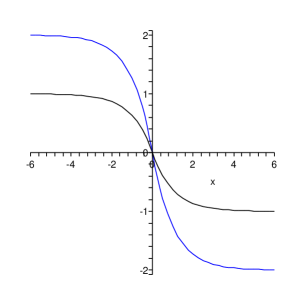
Figure 1: The weak kink solution at $t=0$. Black line: $u(x,0)$; Blue line: $v(x,0)$.

Acknowledgments  Qiao was partially supported by the Texas Norman Hackerman Advanced Research Program (Grant No. 003599-0001-2009) and supervised the U.S. Department of Education UTPA-GAANN program (P200A120256). Yin was partially supported by NNSFC (No. 11271382), RFDP (No. 20120171110014), and the key project of Sun Yat-sen University (No. c1185).

References

[1]
Bahouri, H., Chemin, J.-Y., and Danchin, R., Fourier Analysis and Nonlinear Partial Differential Equations,
Grundlehren der MathematischenWissenschaften, Vol. 343, Berlin-Heidelberg-NewYork: Springer, 2011.
[2]
Beals, R., Sattinger, D. and Szmigielski, J., Acoustic scattering
and the extended Korteweg-de Vries hierarchy, Adv. Math.,140 (1998), 190–206.
[3]
Bressan, A. and Constantin, A., Global conservative solutions of the
Camassa-Holm equation, Arch. Rat. Mech. Anal.,183
(2007), 215–239.
[4]
Camassa, R. and Holm, D., An integrable shallow water equation with
peaked solitons, Phys. Rev. Letters,71 (1993),
1661–1664.
[5]
Camassa, R., Holm, D. and Hyman, J., A new integrable shallow water
equation, Adv. Appl. Mech.,31 (1994), 1–33.
[6]
Chen, M., Liu, S-Q. and Zhang, Y., A 2-component generalization of the
Camassa-Holm equation and its solutions, Lett. Math. Phys.,
75 (2006), 1-15.
[7]
Coclite, G. M. and Karlsen, K. H., On the well-posedness of the
Degasperis-Procesi equation, J. Funct. Anal., 233
(2006), 60–91.
[8]
Constantin, A., Global existence of solutions and breaking waves
for a shallow water equation: a geometric approach, Ann.
Inst. Fourier (Grenoble),50 (2000), 321–362.
[9]
Constantin, A., The trajectories of particles in Stokes waves, Invent. Math.,166 (2006),
523–535.
[10]
Constantin, A. and Escher, J., Global existence and blow-up for a
shallow water equation, Annali Sc. Norm. Sup. Pisa,26
(1998), 303–328.
[11]
Constantin, A. and Escher, J., Well-posedness, global existence, and
blowup phenomena for a periodic quasi-linear hyperbolic equation,
Comm. Pure Appl. Math.,51 (1998), 475–504.
[12]
Constantin, A. and Escher, J., Wave breaking for nonlinear nonlocal
shallow water equations, Acta Mathematica,181 (1998), 229–243.
[13]
Constantin, A. and Escher, J., Analyticity of periodic traveling free surface water waves with vorticity,
Ann. of Math. (2),173 (2011), 559–568.
[14]
Constantin, A. and Ivanov, R., On an integrable two-component
Camassa-Holm shallow water system, Phys. Lett. A,372
(2008), 7129–7132.
[15]
Constantin, A., Ivanov, R. and Lenells, J., Inverse scattering
transform for the Degasperis-Procesi equation, Nonlinearity,23 (2010), 2559–2575.
[16]
Constantin, A. and Kolev, B., Geodesic flow on the diffeomorphism group of the circle, Comm. Math. Helv.,78(2003), 787–804.
[17]
Constantin, A. and Lannes, D., The hydrodynamical relevance of the
Camassa-Holm and Degasperis-Procesi equations, Arch. Rat. Mech.
Anal.,192 (2009), 165–186.
[18]
Constantin, A. and Molinet, L., Global weak solutions for a shallow
water equation, Comm. Math. Phys.,211 (2000), 45–61.
[19]
Constantin, A. and Strauss, W. A., Stability of peakons, Comm.
Pure Appl. Math.,53 (2000), 603–610.
[20]
Dai, H. H., Model equations for nonlinear dispersive waves in a
compressible Mooney-Rivlin rod, Acta Mech.127 (1998),
193–207.
[21]
Danchin, R., A few remarks on the Camassa-Holm equation, Differential Integral Equations,14 (2001), 953–988.
[22]
Degasperis, A., Holm, D. D. and Hone, A. N. W., A new integral
equation with peakon solutions, Theo. Math. Phys.,133 (2002), 1463-1474.
[23]
Degasperis, A. and Procesi, M., Asymptotic integrability, Symmetry and Perturbation Theory, Rome, 1998, World Sci. Publishing,
River Edge, NJ, 1999, pp. 23-37.
[24]
Dullin, H. R., Gottwald, G. A. and Holm, D. D., An integrable shallow water equation with linear and nonlinear dispersion, Phys. Rev. Letters,87 (2001), 4501–4504.
[25]
Escher, J. and Kolev, B., The Degasperis-Procesi equation as a non-metric Euler equation, Math. Z.,269 (2011), 1137–1153.
[26]
Escher, J., Lechtenfeld, O., and Yin, Z., Well-posedness and blow-up phenomena for the 2-component Camassa-Holm equation, Discrete Contin. Dyn. Syst., 19 (2007), 493–513.
[27]
Escher, J., Liu, Y. and Yin, Z., Global weak solutions and blow-up
structure for the Degasperis-Procesi equation, J. Funct.
Anal., 241 (2006), 457–485.
[28]
Escher, J., Liu, Y. and Yin, Z., Shock waves and blow-up phenomena
for the periodic Degasperis-Procesi equation,
Indiana Univ. Math. J.,56 (2007), 87–117.
[29]
Escher, J. and Yin, Z., Initial boundary value problems for nonlinear dispersive wave equations,
J. Funct. Anal., 256 (2009), 479–508.
[30]A. Fokas, On a class of physically important integrable
equations, Physica D,87 (1995), 145-150.
[31]
Fokas, A. and Fuchssteiner, B., Symplectic structures, their Bäcklund transformation and hereditary symmetries, Physica D4 (1981), 47–66.
[32]
Fuchssteiner, B., Some tricks from the symmetry-toolbox for nonlinear equations: generalizations of the Camassa-Holm eqaution, Physica D, 95 (1996), 229–243.
[33]
Guan, C. and Yin, Z., Global existence and blow-up phenomena for an
integrable two-component Camassa-Holm shallow water system,
J. Differential Equations, 248 (2010), 2003-2014.
[34]
Guan, C., Karlsen, K.H. and Yin, Z., Well-posedness and blow-up phenomena for a modified two-component Camassa-Holm equation, Contemp. Math.,
526 (2010), 199–220.
[35]
Guan, C. and Yin, Z., Global weak solutions for a two-component Camassa-Holm shallow water system,
J. Funct. Anal., 260 (2011), 1132-1154.
[36]
Guan, C. and Yin, Z., Global weak solutions for a modified two-component Camassa-Holm equation, Annales de l’Institut Henri Poincare (C) Non Linear Analysis, 28 (2011), 623–641.
[37]
Gui, G. and Liu, Y., On the global existence and wave-breaking criteria for the two-component Camassa-Holm system,
J. Funct. Anal., 258 (2010), 4251–4278.
[38]
Gui, G., Liu, Y., Olver, P., and Qu, C., Wave-breaking and peakons for a modified Camassa-Holm equation,
Comm. Math. Phys., 319 (2013), 731–759.
[39]
Himonas, A. A. and Holliman, C., The Cauchy problem for the Novikov equation,
Nonlinearity, 25 (2012), 449–479.
[40]
Holm, D., Naraigh, L. and Tronci, C., Singular solution of a modified
two-component Camassa-Holm equation, Phys. Rev. E(3), 79 (2009), 1-13.
[41]
Hone, A. N. and Wang, J. P., Integrable peakon equations with cubic nonlinearity,
J. Phys. A, 41 (2008), 372002.
[42]
Johnson, R. S., Camassa-Holm, Korteweg-de Vries and related models for water waves, J. Fluid. Mech.457 (2002), 63–82.
[43]
Kato, T., Quasi-linear equations of evolution, with applications to partial differential equations,
in: Spectral Theory and Differential Equations, Lecture Notes in Math., Springer Verlag, Berlin,
448 (1975), 25–70.
[44]
Liu, Y. and Yin, Z., Global existence and blow-up phenomena for the
Degasperis-Procesi equation, Comm. Math. Phys.,267 (2006), 801–820.
[45]
Lundmark, H., Formation and dynamics of shock waves in the Degasperis-Procesi equation,
J. Nonlinear Sci.,17 (2007), 169–198.
[46]
Novikov, V., Generalizations of the Camassa-Holm equation, J. Phys. A,42 (2009) 342002.
[47]
Olver, P. J. and Rosenau P., Tri-Hamiltonian duality between solitons and solitary-wave solutions having compact support, Phys. Rev. E,53 (1996) 1900–1906.
[48]
Popowicz, Z., A two-component generalization of the Degasperis-Procesi equation,
J. Phys. A: Math. Gen.,39 (2006), 13717–13726.
[49]
Qiao, Z., The Camassa-Holm hierarchy, N-dimensional integrable systems, and algebro-geometric solution on a symplectic submanifold, Comm. Math. Phys.,239 (2003), 309–341.
[50]
Qiao, Z., A new integrable equation with cuspons and W/M-shape-peaks solitons,
J. Math. Phys.,47 (2006), 112701.
[51]
Qiao, Z. and Li, X., An integrable equation with nonsmooth solitons,
Theor. Math. Phys.,267 (2011), 584–589.
[52]
Qiao, Z., Xia, B., and Li, J., Integrable system with peakon, weak kink, and kink-peakon interactional solutions, arXiv:1205.2028v2.
[53]
Tan, W. and Yin, Z., Global periodic conservative solutions of a periodic modified two-component Camassa-Holm equation, J. Funct. Anal., 261 (2011), 1204–1226.
[54]
Whitham, G. B., Linear and Nonlinear Waves, J. Wiley & Sons, New York, 1980.
[55]
Wu, X. and Yin, Z., Global weak solutions for the Novikov equation,
J. Phys. A,44 (2011), 055202.
[56]
Xia, B. and Qiao, Z., A new two-component integrable system with peakon and weak kink solutions, arXiv:1211.5727v2.
[57]
Xin, Z. and Zhang, P., On the weak solutions to a shallow water
equation, Comm. Pure Appl. Math.,53 (2000),
1411–1433.
[58]
Yan, K. and Yin, Z., Analytic solutions of the Cauchy problem for two-component shallow water systems,
Math. Z.,269 (2011), 1113–1127.
[59]
Yan, K. and Yin, Z., On the Cauchy problem for a two-component Degasperis-Procesi system,
J. Differential Equations,252 (2012), 2131–2159.
[60]
Yan, K. and Yin, Z., Well-posedness for a modified two-component Camassa-Holm system in critical spaces,
Discrete Contin. Dyn. Syst.,33 (2013), 1699–1712.
[61]
Yan, K. and Yin, Z., Initial boundary value problems for the
two-component shallow water systems, Rev. Mat.
Iberoamericana, (2013), in press.
[62]
Yin, Z., On the Cauchy problem for an integrable equation with
peakon solutions, Illinois J. Math.,47 (2003),
649–666.
[63]
Yin, Z., Global weak solutions to a new periodic integrable
equation with peakon solutions, J. Funct. Anal.,212
(2004), 182–194.