Anisotropic effective higher-order response of heterogeneous Cauchy elastic materials

Abstract

The homogenization results obtained by Bacca et al. (Homogenization of heterogeneous Cauchy-elastic materials leads to Mindlin second-gradient elasticity. Part I: Closed form expression for the effective higher-order constitutive tensor. http://arxiv.org/abs/1305.2365 Submitted, 2013), to define effective second-gradient elastic materials from heterogeneous Cauchy elastic solids, are extended here to the case of phases having non-isotropic tensors of inertia. It is shown that the nonlocal constitutive tensor for the homogenized material depends on both the inertia properties of the RVE and the difference between the effective and the matrix local elastic tensors. Results show that: (i.) a composite material can be designed to result locally isotropic but nonlocally orthotropic; (ii.) orthotropic nonlocal effects are introduced when a dilute distribution of aligned elliptical holes and, in the limit case, of cracks is homogenized.

Keywords: Second-order homogenization; Higher-order elasticity; Effective nonlocal continuum; Characteristic length-scale; Cracked materials.

1 Introduction

Microstructures introduce length-scales and nonlocal effects in the mechanical modeling of solids, so that the use of higher-order theories becomes imperative, in particular when large strain gradients are involved [as in the case of localization of deformation (Dal Corso and Willis, 2011) or fracture mechanics (Mishuris et al., 2012)].

Nonlocality, often introduced phenomenologically (Cosserat and Cosserat, 1909; Koiter, 1964; Mindlin, 1964; Aifantis, 1978), can be analyzed from the fundamental and scarcely explored point of view in which it is linked to the microstructure of a Cauchy elastic heterogeneous material via homogenization theory. This approach was followed by Bigoni and Drugan (2007) and extended by Bacca et al. (2013a) who obtained a closed-form solution for the nonlocal effective response through a second-order homogenization procedure, based on the dilute approximation. In the present article this result is generalized to allow the possibility of phases having non-spherical ellipsoids of inertia (or non-circular ellipses of inertia in plane strain), Fig. 1, left.

Figure 1: Heterogeneous Cauchy material (left) made up of an inclusion phase with constitutive tensor $\mbox{\boldmath${\mathsf{C}}$}^{(2)}$ embedded within a matrix with constitutive tensor $\mbox{\boldmath${\mathsf{C}}$}^{(1)}$ and homogeneous equivalent SGE material (right) with effective tensors $\mbox{\boldmath${\mathsf{C}}$}^{eq}$ and $\mbox{\boldmath${\mathsf{A}}$}^{eq}$.

By matching the elastic energy of a Cauchy elastic heterogeneous material (Fig. 1, left) with that of a homogeneous higher-order elastic solid (Fig. 1, right), both subject to the same displacement conditions on the boundary, it is shown that a sixth-order constitutive tensor can be obtained, defining a second-gradient elastic (SGE) material (Mindlin, 1964). The results show how the shape and the constitutive symmetry class of the phases influence the higher-order response and are exploited to investigate two particular cases of special interest. One case is that a Cauchy elastic heterogeneous material (e.g. a rectangular lattice of circular elastic inclusions in an isotropic elastic matrix, Fig. 2, right) can be designed to result at the same time locally isotropic, but nonlocally orthotropic.

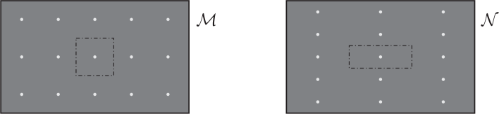
Figure 2: Two composites $\mathcal{M}$ and $\mathcal{N}$ containing a dilute suspension of isotropic circular inclusions in an isotropic matrix (with the same volume ratio $f\ll 1$). While standard homogenization leads to the same effective isotropic constitutive fourth-order tensor for both distributions, $\mbox{\boldmath${\mathsf{C}}$}^{eq}(\mathcal{M})=\mbox{\boldmath${\mathsf{C}}$}^{eq}(\mathcal{N})$, second-order homogenization leads to different effective nonlocal properties, $\mbox{\boldmath${\mathsf{A}}$}^{eq}(\mathcal{M})\neq\mbox{\boldmath${\mathsf{A}}$}^{eq}(\mathcal{N})$. In particular, while $\mbox{\boldmath${\mathsf{A}}$}^{eq}(\mathcal{M})$ is isotropic, $\mbox{\boldmath${\mathsf{A}}$}^{eq}(\mathcal{N})$ is orthotropic.

The other one is the case of a dilute distribution of aligned elliptical voids and the limit case of cracks, providing nonlocal orthotropic effects.

2 Nonlocal effective response

Through application of the second-order homogenization procedure, the evaluation of the effective nonlocal response of a Second Gradient Elastic solid (Mindlin, 1964) obtained by Bacca et al. (2013a), and valid for a RVE having inclusion and matrix with spherical ellipsoids of inertia, is extended to the case of phases with generic ellipsoid of inertia.

The homogenization is performed on a heterogeneous Cauchy RVE (volume $\Omega_{RVE}^{C}$; Fig. 1, left), where a dilute distribution of inclusions (phase (2), local constitutive tensor $\mbox{\boldmath${\mathsf{C}}$}^{(2)}$, volume $\Omega_{2}^{C}$=$f\Omega_{RVE}^{C}$, volume fraction $f\ll 1$) is embedded within a matrix (phase (1), local constitutive tensor $\mbox{\boldmath${\mathsf{C}}$}^{(1)}$ volume $\Omega_{1}^{C}$=$(1-f)\Omega_{RVE}^{C}$). The homogenization leads to a homogeneous SGE material (with effective local constitutive tensor $\mbox{\boldmath${\mathsf{C}}$}^{eq}$ and nonlocal constitutive tensor $\mbox{\boldmath${\mathsf{A}}$}^{eq}$, volume $\Omega_{eq}^{SGE}=\Omega_{RVE}^{C}$; Fig. 1, right). The equivalent response is obtained through the annihilation of the strain energy mismatch between the heterogeneous and equivalent materials, which is

$$\mathcal{W}_{RVE}^{C}\left(\mbox{\boldmath${\mathsf{C}}$}^{(1)},\mbox{\boldmath${\mathsf{C}}$}^{(2)}\right)-\mathcal{W}_{eq}^{SGE}\left(\mbox{\boldmath${\mathsf{C}}$}^{eq},\mbox{\boldmath${\mathsf{A}}$}^{eq}\right)=0,$$ (1)

when the following second-order (linear and quadratic) displacement field $\overline{\mbox{\boldmath${\it u}$}}$ is imposed on both the boundaries of the RVE and the SGE

$$\mbox{\boldmath${\it u}$}=\overline{\mbox{\boldmath${\it u}$}},~{}~{}~{}\mbox{on }\partial\Omega_{RVE}^{C},\qquad\mbox{and}\qquad\left\{\begin{array}[]{lll}\mbox{\boldmath${\it u}$}=\overline{\mbox{\boldmath${\it u}$}},\\[11.38109pt] D\mbox{\boldmath${\it u}$}=D\overline{\mbox{\boldmath${\it u}$}},\end{array}\right.~{}~{}~{}\mbox{on }\partial\Omega_{eq}^{SGE},$$ (2)

with

$$\overline{u}_{i}=\underbrace{\alpha_{ij}x_{j}}_{\displaystyle\overline{u}_{i}^{\alpha}}+\underbrace{\beta_{ijk}x_{j}x_{k}}_{\displaystyle\overline{u}_{i}^{\beta}},$$ (3)

where $\alpha_{ij}$ and $\beta_{ijk}$ are constant coefficients, the latter satisfying the symmetry $\beta_{ijk}$=$\beta_{ikj}$. The strain energies for the heterogeneous Cauchy material and the equivalent SGE material are given by integration over the domain of the respective strain energy density, namely

$$\begin{array}[]{lll}\mathcal{W}_{RVE}^{C}=\displaystyle\frac{1}{2}\int_{\Omega_{1}^{C}}\mbox{\boldmath${\mathsf{C}}$}^{(1)}_{ijhk}u_{i,j}u_{h,k}+\frac{1}{2}\int_{\Omega_{2}^{C}}\mbox{\boldmath${\mathsf{C}}$}^{(2)}_{ijhk}u_{i,j}u_{h,k},\\[14.22636pt] \mathcal{W}_{eq}^{SGE}=\displaystyle\frac{1}{2}\int_{\Omega_{eq}^{SGE}}\left[\mbox{\boldmath${\mathsf{C}}$}^{eq}_{ijhk}u_{i,j}u_{h,k}+\mbox{\boldmath${\mathsf{A}}$}^{eq}_{ijklmn}u_{k,ij}u_{n,lm}\right].\end{array}$$ (4)

To explicitly evaluate the effective nonlocal response, some of the geometrical assumptions introduced by Bacca et al. (2013a) are now modified. In particular, coincidence of the centroids of matrix and inclusion, both centered at the origin of the $x_{i}$–axes (i.e. geometrical property GP1 in Bacca et al. 2013a) is still assumed, namely, the static moment vectors of the inclusion, of the matrix and of the RVE are null

$$\mbox{\boldmath${\it S}$}(\Omega_{1}^{C})=\mbox{\boldmath${\it S}$}(\Omega_{2}^{C})=\mbox{\boldmath${\it S}$}(\Omega_{RVE}^{C})=\mbox{\boldmath${0}$},\qquad\mbox{\boldmath${\it S}$}(V)=\int_{V}\mbox{\boldmath${\it x}$},$$ (5)

but no restriction is now assumed about the shape and the directions of the ellipsoids of inertia for matrix and the inclusion (i.e. the geometrical property GP2 of Bacca et al. 2013a is removed).

Introducing the normalized inertia tensor ${\it B}$ for a generic solid occupying the region $V$, defined as the second-order Euler tensor of inertia ${\it E}$ divided by the RVE volume (or area in plane-strain) $\Omega_{RVE}^{C}$,

$$\mbox{\boldmath${\it B}$}(V)=\frac{\mbox{\boldmath${\it E}$}(V)}{\Omega_{RVE}^{C}},\qquad\mbox{\boldmath${\it E}$}(V)=\int_{V}\mbox{\boldmath${\it x}$}\,\otimes\,\mbox{\boldmath${\it x}$},$$ (6)

the normalized tensors of inertia for the matrix $\mbox{\boldmath${\it B}$}^{(1)}=\mbox{\boldmath${\it B}$}(\Omega_{1}^{C})$, the inclusion $\mbox{\boldmath${\it B}$}^{(2)}=\mbox{\boldmath${\it B}$}(\Omega_{2}^{C})$ and the RVE $\mbox{\boldmath${\it B}$}^{RVE}=\mbox{\boldmath${\it B}$}(\Omega_{RVE}^{C})$ are given by

$$\begin{array}[]{lll}\displaystyle\mbox{\boldmath${\it B}$}^{(1)}=(1-f)\sum_{k=1}^{N}\left[\rho_{k}^{(1)}\right]^{2}\,\mbox{\boldmath${\it e}$}_{[k]}^{(1)}\otimes\mbox{\boldmath${\it e}$}_{[k]}^{(1)},\\ \displaystyle\mbox{\boldmath${\it B}$}^{(2)}=f\sum_{k=1}^{N}\left[\rho_{k}^{(2)}\right]^{2}\,\mbox{\boldmath${\it e}$}_{[k]}^{(2)}\otimes\mbox{\boldmath${\it e}$}_{[k]}^{(2)},\\ \displaystyle\mbox{\boldmath${\it B}$}^{RVE}=\sum_{k=1}^{N}\left[\rho_{k}^{RVE}\right]^{2}\,\mbox{\boldmath${\it e}$}_{[k]}^{RVE}\otimes\mbox{\boldmath${\it e}$}_{[k]}^{RVE},\end{array}$$ (7)

where $\left\{\mbox{\boldmath${\it e}$}_{[k]}^{(1)},\mbox{\boldmath${\it e}$}_{[k]}^{(2)},\mbox{\boldmath${\it e}$}_{[k]}^{RVE}\right\}$ are the $k$-th unit vectors identifying the principal system for the matrix, the inclusion, and the RVE, and $\left\{\rho_{k}^{(1)},\rho_{k}^{(2)},\rho_{k}^{RVE}\right\}$ are the respective radii of gyration, and $N$ is equal to 3 (or 2 for plane strain case).

Note that from eqns (6) and (7) it follows

$$\mbox{\boldmath${\it B}$}^{RVE}=\mbox{\boldmath${\it B}$}^{(1)}+\mbox{\boldmath${\it B}$}^{(2)},$$ (8)

so that the normalized tensors of inertia for the RVE can be isotropic, $\mbox{\boldmath${\it B}$}^{RVE}=\left(\rho^{RVE}\right)^{2}\mbox{\boldmath${\it I}$}$, even when the tensors of inertia of the matrix and inclusion are not isotropic. In other words, since $\mbox{\boldmath${\it B}$}^{(1)}$, $\mbox{\boldmath${\it B}$}^{(2)}$ and $\mbox{\boldmath${\it B}$}^{RVE}$ are geometrical quantities, $\mbox{\boldmath${\it B}$}^{RVE}$ corresponds to the normalized inertia of the region enclosed by the the external contour of the RVE.

Considering the normalized inertia tensors (7), it is assumed that for the inclusion all the radii of gyration $\rho_{k}^{(2)}$ vanish in the limit of null inclusion volume fraction $f$ (a modification of the geometrical property GP3 in Bacca et al. 2013a), namely,

$$\lim_{f\rightarrow 0}\rho_{k}^{(2)}(f)=0,\qquad\forall\,\,k=1,...,N.$$ (9)

Similarly to the computations in (Bacca et al., 2013a), the energy mismatch condition (1) is now used to obtain a nonlocal material equivalent to the heterogeneous Cauchy RVE. Since Lemmas 1 and 2 in (Bacca et al., 2013a) are not affected by the geometrical assumption GP2 (which is now removed), the mutual energy is still null at first-order in $f$. Considering that $\mbox{\boldmath${\mathsf{C}}$}^{eq}$ is obtained through a first-order homogenization, the energy mismatch (1) is given only by the contribution related to the sole quadratic displacement boundary condition,

$$\mathcal{W}_{RVE}^{C}(\overline{\mbox{\boldmath${\it u}$}})-\mathcal{W}_{eq}^{SGE}(\overline{\mbox{\boldmath${\it u}$}},D\overline{\mbox{\boldmath${\it u}$}})=\mathcal{W}_{RVE}^{C}(\overline{\mbox{\boldmath${\it u}$}}^{\beta^{\diamond*}})-\mathcal{W}_{eq}^{SGE}(\overline{\mbox{\boldmath${\it u}$}}^{\beta^{\diamond*}},D\overline{\mbox{\boldmath${\it u}$}}^{\beta^{\diamond*}})+o(f),$$ (10)

where the symbol $\diamond$ denotes the fact that the quadratic displacement field is restricted to produce a self-equilibrated stress in an auxiliary homogeneous medium with local tensor $\mbox{\boldmath${\mathsf{C}}$}^{*}$, taken as a first-order perturbation in $f$ to the equivalent local constitutive tensor $\mbox{\boldmath${\mathsf{C}}$}^{eq}$ (see Bacca et al., 2013a, for details).

Lemmas 3 and 4 in (Bacca et al., 2013a) can be extended by considering the definition of normalized Euler tensors of inertia given by eqns (7), and from which the strain energies instrumental to compute the energy mismatch can be obtained as

$$\mathcal{W}_{RVE}^{C}(\overline{\mbox{\boldmath${\it u}$}}^{\beta^{\diamond*}})=2\Omega_{RVE}^{C}B_{lm}^{RVE}\mbox{\boldmath${\mathsf{C}}$}^{(1)}_{ijhk}\beta^{\diamond*}_{ijl}\beta^{\diamond*}_{hkm}+o(f),$$ (11)

and

$$\mathcal{W}_{eq}^{SGE}(\overline{\mbox{\boldmath${\it u}$}}^{\beta^{\diamond*}},D\overline{\mbox{\boldmath${\it u}$}}^{\beta^{\diamond*}})=2\Omega_{RVE}^{C}\left(B_{lm}^{RVE}\mbox{\boldmath${\mathsf{C}}$}^{eq}_{ijhk}+\mbox{\boldmath${\mathsf{A}}$}^{eq}_{jlikmh}\right)\beta^{\diamond*}_{ijl}\beta^{\diamond*}_{hkm}+o(f).$$ (12)

By using eqns (11) and (12) to impose the annihilation of the energy mismatch (1) for a generic purely quadratic boundary condition (and leading to a self-equilibrated stress within the arbitrary medium characterized by local tensor $\mbox{\boldmath${\mathsf{C}}$}^{*}$), the nonlocal sixth-order tensor $\mbox{\boldmath${\mathsf{A}}$}^{eq}$ of the equivalent SGE material is evaluated (at first-order in $f$) as

$$\boxed{\begin{split}\mbox{\boldmath${\mathsf{A}}$}^{eq}_{ijhlmn}&=-\frac{f}{4}\left(\tilde{\mbox{\boldmath${\mathsf{C}}$}}_{ihln}B_{jm}^{RVE}+\tilde{\mbox{\boldmath${\mathsf{C}}$}}_{ihmn}B_{jl}^{RVE}+\tilde{\mbox{\boldmath${\mathsf{C}}$}}_{jhln}B_{im}^{RVE}+\tilde{\mbox{\boldmath${\mathsf{C}}$}}_{jhmn}B_{il}^{RVE}\right),\end{split}}$$ (13)

where $\tilde{\mbox{\boldmath${\mathsf{C}}$}}$ is the first-order discrepancy tensor, defined as

$$\mbox{\boldmath${\mathsf{C}}$}^{eq}=\mbox{\boldmath${\mathsf{C}}$}^{(1)}+f\tilde{\mbox{\boldmath${\mathsf{C}}$}},$$ (14)

and assumed to be known from standard homogenization.

Solution (13) represents the evaluation –in the dilute case– of the nonlocal behaviour of the equivalent SGE material under the geometrical assumptions (5) and (9). Regardless of the ellipsoid of inertia of the inclusion phase, this solution reduces to that given in (Bacca et al., 2013a) when a RVE enclosing a region with a spherical ellipsoid of inertia, $B_{ij}^{RVE}=\left(\rho^{RVE}\right)^{2}\delta_{ij}$, is considered

$$\begin{split}\mbox{\boldmath${\mathsf{A}}$}^{eq}_{ijhlmn}&=-f\frac{\left(\rho^{RVE}\right)^{2}}{4}\left(\tilde{\mbox{\boldmath${\mathsf{C}}$}}_{ihln}\delta_{jm}+\tilde{\mbox{\boldmath${\mathsf{C}}$}}_{ihmn}\delta_{jl}+\tilde{\mbox{\boldmath${\mathsf{C}}$}}_{jhln}\delta_{im}+\tilde{\mbox{\boldmath${\mathsf{C}}$}}_{jhmn}\delta_{il}\right).\end{split}$$ (15)

It is worth to remark that, while the normalized inertia tensor $\mbox{\boldmath${\it B}$}^{RVE}$ is dependent only on the shape and size of the external boundary of the RVE, the first-order discrepancy tensor $\tilde{\mbox{\boldmath${\mathsf{C}}$}}$ is dependent on the constitutive tensors of both phases and on the shape of the inclusion phase.

Similarly to the case of phases with spherical ellipsoid of inertia (Bacca et al., 2013b), it can be noted that:

• the equivalent SGE material is positive definite if and only if $\tilde{\mbox{\boldmath${\mathsf{C}}$}}$ is negative definite;

• the constitutive higher-order tensor $\mbox{\boldmath${\mathsf{A}}$}^{eq}$ is linear in $f$ for dilute concentrations;

but, differently, the higher-order material symmetries of the equivalent SGE solid involves not only the material symmetries of the first-order discrepancy tensor $\tilde{\mbox{\boldmath${\mathsf{C}}$}}$. Indeed, when a RVE encloses a region with a non-spherical ellipsoid of inertia (see Appendix A for details),

the symmetry class of the higher-order response for the effective material coincides with the symmetry class of both the RVE’s normalized inertia tensor $\mbox{\boldmath${\it B}$}^{RVE}$ and the first-order discrepancy tensor $\tilde{\mbox{\boldmath${\mathsf{C}}$}}$.

Therefore it is transparent that an isotropic higher-order behaviour (in the dilute case) is obtained only when both the first-order discrepancy tensor $\tilde{\mbox{\boldmath${\mathsf{C}}$}}$ and the normalized inertia tensor $\mbox{\boldmath${\it B}$}^{RVE}$ are isotropic.

3 Application cases

With reference to composites with phases having isotropic Cauchy behaviour

$$\mbox{\boldmath${\mathsf{C}}$}^{(1)}_{ijhk}\displaystyle=\lambda_{1}\delta_{ij}\delta_{hk}+\mu_{1}(\delta_{ih}\delta_{jk}+\delta_{ik}\delta_{jh}),\qquad\displaystyle\mbox{\boldmath${\mathsf{C}}$}^{(2)}_{ijhk}\displaystyle=\lambda_{2}\delta_{ij}\delta_{hk}+\mu_{2}(\delta_{ih}\delta_{jk}+\delta_{ik}\delta_{jh}),$$ (16)

the anisotropic nonlocal effective response is analyzed by considering applications of the homogenization result (13) to the following specific geometries:

• RVE enclosing a region with a spherical ellipsoid of inertia;

• inclusion with non-spherical ellipsoid of inertia.

The above examples show that, similarly to the usual first-order homogenization, specific assumptions on the geometry of the phases lead to anisotropic nonlocal effective response and that, more interestingly, in the case of RVE enclosing a region with non-spherical ellipsoid inertia (and under the dilute assumption), anisotropic nonlocal effective response can arise even in composites having isotropic local effective behaviour.

3.1 RVE enclosing a region with non-spherical ellipsoid inertia

Restricting attention to inclusions which geometry is such that the first-order discrepancy tensor, eqn (14), is isotropic

$$\tilde{\mbox{\boldmath${\mathsf{C}}$}}_{ijhk}\displaystyle=\tilde{\lambda}\delta_{ij}\delta_{hk}+\tilde{\mu}(\delta_{ih}\delta_{jk}+\delta_{ik}\delta_{jh}),$$ (17)

and considering the principal directions of the RVE ellipsoid of inertia as the reference system, the components of the normalized tensor of inertia $\mbox{\boldmath${\it B}$}^{RVE}$, eqn (7)₃, can be written as

$$B^{RVE}_{ij}=\sum_{k=1}^{N}\left(\rho^{RVE}_{k}\right)^{2}\delta_{ik}\delta_{jk},$$ (18)

and the solution (13) leads to the following effective nonlocal orthotropic tensor

$$\begin{array}[]{lll}\mbox{\boldmath${\mathsf{A}}$}^{eq}_{ijhlmn}=\displaystyle\sum_{k=1}^{N}&\displaystyle\left\{\frac{a_{2}^{[k]}}{2}\left(\delta_{ih}\delta_{kj}+\delta_{jh}\delta_{ki}\right)\left(\delta_{ln}\delta_{km}+\delta_{mn}\delta_{kl}\right)\right.\\[8.53581pt] &\displaystyle\left.+\frac{a_{4}^{[k]}}{2}\delta_{hn}\left[\delta_{kj}\left(\delta_{im}\delta_{kl}+\delta_{il}\delta_{km}\right)+\delta_{ki}\left(\delta_{jl}\delta_{km}+\delta_{jm}\delta_{kl}\right)\right]\right.\\[8.53581pt] &\displaystyle\left.+\frac{a_{5}^{[k]}}{2}\left[\delta_{in}\delta_{kj}\left(\delta_{hl}\delta_{km}+\delta_{hm}\delta_{kl}\right)+\delta_{jn}\delta_{ki}\left(\delta_{hm}\delta_{kl}+\delta_{hl}\delta_{km}\right)\right]\right\},\end{array}$$ (19)

where the $3N$ nonlocal parameters are given by

$$a_{2}^{[k]}=-f\frac{\left(\rho^{RVE}_{k}\right)^{2}}{2}\tilde{\lambda},\qquad a_{4}^{[k]}=a_{5}^{[k]}=-f\frac{\left(\rho^{RVE}_{k}\right)^{2}}{2}\tilde{\mu},\qquad k=1,...,N.$$ (20)

Note that the effective nonlocal tensor $\mbox{\boldmath${\mathsf{A}}$}^{eq}$, eqn (19), is an orthotropic sixth-order tensor and that it reduces to an isotropic sixth-order tensor when the ellipsoid of inertia of the RVE becomes a sphere (or a circle in plane strain), $\rho_{k}^{RVE}=\rho^{RVE}$ for $k=1,...,N$. Furthermore, the homogenization procedure leads to a positive definite SGE material when the discrepancy tensor $\tilde{\mbox{\boldmath${\mathsf{C}}$}}$ is negative definite, corresponding to

$$\begin{array}[]{c}\tilde{K}<0,~{}~{}~{}\tilde{\mu}<0,\end{array}$$ (21)

where $\tilde{K}$ is the bulk modulus, equal to $\tilde{\lambda}+2\tilde{\mu}/3$ when $N=3$ and $\tilde{\lambda}+\tilde{\mu}$ when $N=2$.

It is worth to mention that the $3(N-1)$ nonlocal parameters $\left\{a_{2}^{[k]};a_{4}^{[k]};a_{5}^{[k]}\right\}$ ($k=2,N$) can be expressed as functions of the two nonlocal parameters $\left\{a_{2}^{[1]};a_{4}^{[1]}\right\}$ as

$$\begin{array}[]{lll}\displaystyle a_{2}^{[k]}=\left(\frac{\rho^{RVE}_{k}}{\rho_{1}^{RVE}}\right)^{2}a_{2}^{[1]},\qquad a_{4}^{[k]}=a_{5}^{[k]}=\left(\frac{\rho^{RVE}_{k}}{\rho_{1}^{RVE}}\right)^{2}a_{4}^{[1]},\qquad\qquad k=2,N.\end{array}$$ (22)

Equation (22) reveals that (for inclusions less stiff than the matrix and) if $\rho^{RVE}_{k}/\rho_{1}^{RVE}>1$ ($<1$), namely, when the distance between the inclusions is larger (smaller) in the direction $k$ than in direction 1, then the nonlocal behaviour is stiffer (less stiff) in the former direction than in the latter (Fig. 2, right).

The explicit evaluation of the non-local parameters is provided below for two simple cases, by considering the discrepancy parameters $\tilde{\lambda}$ and $\tilde{\mu}$ reported in (Bacca et al., 2013b), since the first-order homogenization result is not affected by the external shape of the RVE in the dilute case.

Circular elastic inclusion within a rectangular RVE.

In the case of a circular elastic inclusion (in plane strain condition) of radius $r$ embedded in a rectangular RVE with edges $h_{1}$ and $h_{2}$ (parallel to the directions $x_{k}$, $k=1,2$), the three nonlocal parameters $\left\{a_{2}^{[1]};a_{4}^{[1]};a_{5}^{[1]}\right\}$ are obtained through eqn (20) as

$$\begin{array}[]{lll}\displaystyle a_{2}^{[1]}=\frac{\pi r^{2}}{24}\frac{h_{1}}{h_{2}}\left[\frac{(K_{1}-K_{2})(K_{1}+\mu_{1})}{K_{2}+\mu_{1}}-\frac{\mu_{1}(\mu_{1}-\mu_{2})(K_{1}+\mu_{1})}{2\mu_{1}\mu_{2}+K_{1}(\mu_{1}+\mu_{2})}\right],\\[14.22636pt] \displaystyle a_{4}^{[1]}=a_{5}^{[1]}=\frac{\pi r^{2}}{24}\frac{h_{1}}{h_{2}}\frac{\mu_{1}(\mu_{1}-\mu_{2})(K_{1}+\mu_{1})}{2\mu_{1}\mu_{2}+K_{1}(\mu_{1}+\mu_{2})},\end{array}$$ (23)

from which, by using relation (22), the remaining three parameters $\left\{a_{2}^{[2]};a_{4}^{[2]};a_{5}^{[2]}\right\}$ follow in the form

$$a_{2}^{[2]}=\left(\frac{h_{2}}{h_{1}}\right)^{2}a_{2}^{[1]},\qquad a_{4}^{[2]}=a_{5}^{[2]}=\left(\frac{h_{2}}{h_{1}}\right)^{2}a_{4}^{[1]}.$$ (24)

Note that a positive definite equivalent SGE material is obtained only when the inclusion phase is ‘softer’ than the matrix in terms of both shear and bulk moduli, namely,

$$\mu_{2}<\mu_{1},\qquad K_{2}<K_{1}.$$ (25)

Spherical inclusion within a parallelepipedic RVE.

In the case of a spherical elastic inclusion of radius $r$ embedded in a parallelepiped with sides $h_{1}$, $h_{2}$ and $h_{3}$ (parallel to the directions $x_{k}$, $k=1,2,3$), the three nonlocal parameters $\left\{a_{2}^{[1]};a_{4}^{[1]};a_{5}^{[1]}\right\}$ are obtained through eqn (20) as

$$\begin{array}[]{lll}\displaystyle a_{2}^{[1]}=\frac{\pi r^{3}}{18}\frac{h_{1}}{h_{2}h_{3}}\left[\frac{(3K_{1}+4\mu_{1})(K_{2}-K_{1})}{3K_{2}+4\mu_{1}}-\frac{2}{3}\frac{5\mu_{1}(\mu_{2}-\mu_{1})(3K_{1}+4\mu_{1})}{\mu_{1}(3K_{1}+4\mu_{2})+2(3K_{1}+4\mu_{1})(\mu_{2}+\mu_{1})}\right],\\[14.22636pt] \displaystyle a_{4}^{[1]}=a_{5}^{[1]}=\frac{\pi r^{3}}{18}\frac{h_{1}}{h_{2}h_{3}}\frac{5\mu_{1}(\mu_{2}-\mu_{1})(3K_{1}+4\mu_{1})}{\mu_{1}(3K_{1}+4\mu_{2})+2(3K_{1}+4\mu_{1})(\mu_{2}+\mu_{1})},\end{array}$$ (26)

from which, by using relation (22), the remaining six parameters $\left\{a_{2}^{[2]};a_{4}^{[2]};a_{5}^{[2]};a_{2}^{[3]};a_{4}^{[3]};a_{5}^{[3]}\right\}$ follow in the form

$$\begin{array}[]{lll}\displaystyle a_{2}^{[2]}=\left(\frac{h_{2}}{h_{1}}\right)^{2}a_{2}^{[1]},\qquad a_{4}^{[2]}=a_{5}^{[2]}=\left(\frac{h_{2}}{h_{1}}\right)^{2}a_{4}^{[1]},\qquad\displaystyle a_{2}^{[3]}=\left(\frac{h_{3}}{h_{1}}\right)^{2}a_{2}^{[1]},\qquad a_{4}^{[3]}=a_{5}^{[3]}=\left(\frac{h_{2}}{h_{1}}\right)^{2}a_{4}^{[1]}.\end{array}$$ (27)

Similarly to the case of circular elastic inclusions, the equivalent SGE material is positive definite only when condition (25) is satisfied.

3.2 Inclusion with non-spherical ellipsoid inertia

It has been shown that solution (15), obtained by Bacca et al. (2013a), remains valid regardless of the ellipsoid of inertia of the inclusions, whenever the RVE encloses a region with a spherical ellipsoid of inertia. Solution (15) is now exploited to achieve the nonlocal effective behaviour of a composite with aligned elliptical holes and, in the limit of vanishing ellipse axes ratio, of cracks.

Elliptical hole within an isotropic matrix.

The presence of equally-oriented inclusions with non-spherical ellipsoid of inertia within a composite introduces an anisotropy in the effective behaviour. In particular, when a system of dilute aligned elliptic holes (with semi-axis $b_{k}$ parallel to direction $x_{k}$, $k=1,2$) is considered within an isotropic matrix, the effective behaviour is orthotropic with orthotropy axes coincident with those of the elliptical hole, so that the first-order discrepancy tensor $\tilde{\mbox{\boldmath${\mathsf{C}}$}}$ described in the reference system of orthotropy is (Tsukrov and Kachanov, 2000)

$$\begin{array}[]{lll}\displaystyle\tilde{\mbox{\boldmath${\mathsf{C}}$}}_{ijhk}\displaystyle=&\tilde{\lambda}\delta_{ij}\delta_{hk}+\tilde{\mu}(\delta_{ih}\delta_{jk}+\delta_{ik}\delta_{jh})+\tilde{\xi}\left(\delta_{i1}\delta_{j2}+\delta_{i2}\delta_{j1}\right)\left(\delta_{h1}\delta_{k2}+\delta_{h2}\delta_{k1}\right)+\tilde{\omega}\delta_{i1}\delta_{j1}\delta_{h1}\delta_{k1},\end{array}$$ (28)

with

$$\begin{array}[]{rl}\tilde{\lambda}&\displaystyle=-(\lambda_{1}+2\mu_{1})\frac{\lambda_{1}\left(\lambda_{1}+2\mu_{1}\right)\left(1+\Lambda^{2}\right)-2\Lambda\mu_{1}^{2}}{2\Lambda\mu_{1}(\lambda_{1}+\mu_{1})},\\[11.38109pt] \tilde{\mu}&\displaystyle=-\left(1+\Lambda\right)\left(\lambda_{1}+2\mu_{1}\right)\frac{\lambda_{1}(1-\Lambda)+2\mu_{1}}{2\Lambda\left(\lambda_{1}+\mu_{1}\right)},\\[11.38109pt] \tilde{\xi}&\displaystyle=\left(1-\Lambda^{2}\right)\frac{\lambda_{1}+2\mu_{1}}{2\Lambda},\\[11.38109pt] \tilde{\omega}&\displaystyle=\left(1-\Lambda^{2}\right)\frac{\lambda_{1}+2\mu_{1}}{\Lambda},\end{array}$$ (29)

where the parameter $\Lambda$ is the ratio between the ellipse’s semi-axes, $\Lambda=b_{2}/b_{1}$.

Considering that the RVE encloses a region with a spherical ellipsoid of inertia, $B_{ij}^{RVE}=\left(\rho^{RVE}\right)^{2}\delta_{ij}$, the effective nonlocal tensor $\mbox{\boldmath${\mathsf{A}}$}^{eq}$ can be obtained, exploiting solution (13), as the following positive-definite orthotropic sixth-order tensor

$$\begin{array}[]{llll}\displaystyle\mbox{\boldmath${\mathsf{A}}$}^{eq}_{ijhlmn}=&\displaystyle\frac{a_{2}}{2}\left[\delta_{ih}\left(\delta_{jl}\delta_{mn}+\delta_{jm}\delta_{ln}\right)+\delta_{jh}\left(\delta_{il}\delta_{mn}+\delta_{im}\delta_{ln}\right)\right]\\[8.53581pt] &\displaystyle+a_{4}\left(\delta_{il}\delta_{jm}+\delta_{im}\delta_{jl}\right)\delta_{hn}+\frac{a_{5}}{2}\left[\delta_{in}\left(\delta_{jl}\delta_{hm}+\delta_{jm}\delta_{hl}\right)+\delta_{jn}\left(\delta_{il}\delta_{hm}+\delta_{im}\delta_{hl}\right)\right]\\[8.53581pt] &+\displaystyle\frac{a_{6}}{2}\left\{\left(\delta_{i1}\delta_{h2}+\delta_{i2}\delta_{h1}\right)\left[\left(\delta_{l1}\delta_{n2}+\delta_{l2}\delta_{n1}\right)\delta_{jm}+\left(\delta_{m1}\delta_{n2}+\delta_{m2}\delta_{n1}\right)\delta_{jl}\right]\right.\\[8.53581pt] &\displaystyle\left.+\left(\delta_{j1}\delta_{h2}+\delta_{j2}\delta_{h1}\right)\left[\left(\delta_{l1}\delta_{n2}+\delta_{l2}\delta_{n1}\right)\delta_{im}+\left(\delta_{m1}\delta_{n2}+\delta_{m2}\delta_{n1}\right)\delta_{il}\right]\right\}\\[8.53581pt] &+\displaystyle\frac{a_{9}}{2}\left[\delta_{i1}\left(\delta_{l1}\delta_{jm}+\delta_{m1}\delta_{jl}\right)+\delta_{j1}\left(\delta_{l1}\delta_{im}+\delta_{m1}\delta_{il}\right)\right]\delta_{h1}\delta_{n1},\end{array}$$ (30)

with the following nonlocal parameters

$$\begin{array}[]{ccc}a_{2}=\displaystyle-f\frac{\left(\rho^{RVE}\right)^{2}}{2}\tilde{\lambda},\,\,\,a_{4}=a_{5}=\displaystyle-f\frac{\left(\rho^{RVE}\right)^{2}}{2}\tilde{\mu},\,\,\,a_{6}=\displaystyle-f\frac{\left(\rho^{RVE}\right)^{2}}{2}\tilde{\xi},\,\,\,a_{9}=\displaystyle-f\frac{\left(\rho^{RVE}\right)^{2}}{2}\tilde{\omega}.\end{array}$$ (31)

In the case that the RVE has a square boundary, and by considering the first-order discrepancy quantities given by eqn (29), the nonlocal parameters simplify to

$$\begin{array}[]{lll}a_{2}=\displaystyle\frac{\pi b_{1}^{2}}{48}\frac{\lambda_{1}\left(\lambda_{1}+2\mu_{1}\right)\left(1+\Lambda^{2}\right)-2\Lambda\mu_{1}^{2}}{\mu_{1}(\lambda_{1}+\mu_{1})}(\lambda_{1}+2\mu_{1}),\\[14.22636pt] a_{4}=a_{5}=\displaystyle\frac{\pi b_{1}^{2}}{48}\frac{\lambda_{1}(1-\Lambda)+2\mu_{1}}{\left(\lambda_{1}+\mu_{1}\right)}\left(1+\Lambda\right)\left(\lambda_{1}+2\mu_{1}\right),\\[14.22636pt] a_{6}=\displaystyle-\frac{\pi b_{1}^{2}}{48}\left(1-\Lambda^{2}\right)\left(\lambda_{1}+2\mu_{1}\right),\\[14.22636pt] a_{9}=\displaystyle-\frac{\pi b_{1}^{2}}{24}\left(1-\Lambda^{2}\right)\left(\lambda_{1}+2\mu_{1}\right).\end{array}$$ (32)

The nonlocal effective constants $\left\{a_{2};a_{4}=a_{5};a_{6}=a_{9}/2\right\}$ given by eqn (32) are reported in Fig. 3 as functions of the ellipse semi-axes ratio $b_{2}/b_{1}$ and for different values of the Poisson’s ratio of the matrix $\nu_{1}=\lambda_{1}/(2(\lambda_{1}+\mu_{1}))$. Note that both the constants $a_{6}$ and $a_{9}$, defining the orthotropic nonlocal effective behaviour, approach zero in the limit $b_{2}/b_{1}\rightarrow 1$, so that the nonlocal orthotropic behaviour turns out to be isotropic when the elliptical voids become circular holes.

Effective nonlocal parameters in the limit case of aligned cracks.

Although the sixth-order tensor (30) has been obtained excluding the possibility that inclusions have non-null radius of inertia at null volume ratio (namely, eqn (9)), the nonlocal parameters of the effective tensor $\mbox{\boldmath${\mathsf{A}}$}^{eq}$ for a dilute distribution of aligned ellipses, eqn (32), can be used to obtain the limit values for a dilute distribution of aligned cracks ($\Lambda=b_{2}/b_{1}\rightarrow 0$) with length $2b_{1}$ within a square RVE as

$$a_{2}=\displaystyle\frac{\pi b_{1}^{2}}{48}\frac{\lambda_{1}(\lambda_{1}+2\mu_{1})^{2}}{\mu_{1}(\lambda_{1}+\mu_{1})},\,\,\,a_{4}=a_{5}=\displaystyle\frac{\pi b_{1}^{2}}{48}\frac{\left(\lambda_{1}+2\mu_{1}\right)^{2}}{\lambda_{1}+\mu_{1}},\,\,\,a_{6}=-\displaystyle\frac{\pi b_{1}^{2}}{48}(\lambda_{1}+2\mu_{1}),\,\,\,a_{9}=-\displaystyle\frac{\pi b_{1}^{2}}{24}(\lambda_{1}+2\mu_{1}).$$ (33)

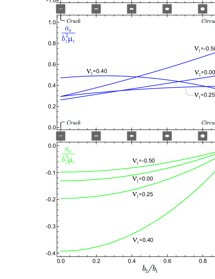
Figure 3: Higher-order constitutive parameters $a_{2}$, $a_{4}=a_{5}$ and $a_{6}=a_{9}/2$ of the SGE solid equivalent to a composite made up of an isotropic matrix containing a dilute suspension of aligned elliptical voids (with major semi-axis $b_{1}$), as functions of the semi-axes ratio $b_{2}/b_{1}$, and for different values of the Poisson’s ratio of the matrix $\nu_{1}$ =$\left\{-0.5;0;0.25;0.4\right\}$. The constants are made dimensionless through division by parameter $b_{1}^{2}\mu_{1}$. Note that both constants $a_{6}$ and $a_{9}$ approach zero in the limit $b_{2}/b_{1}\rightarrow 1$, so that the nonlocal orthotropic behaviour turns out to become isotropic when the elliptical voids become circular holes.

4 Conclusions

An homogenization scheme has been shown to describe nonlocal effects for a heterogeneous Cauchy elastic material containing a dilute distribution of inclusions of arbitrary shape in an arbitrary RVE (under the condition that inclusion and RVE have a coincident center of mass). Results show that the shape of the RVE influences the effective nonlocal behaviour even under the dilute approximation, in contrast with the usual homogenization scheme valid at first-order.

Acknowledgments M. Bacca gratefully acknowledges financial support from Italian Prin 2009 (prot. 2009XWLFKW-002). D. Bigoni, F. Dal Corso and D. Veber gratefully acknowledge financial support from the grant PIAP-GA-2011-286110-INTERCER2, ‘Modelling and optimal design of ceramic structures with defects and imperfect interfaces’.

Appendix A Coincidence of symmetry class of $\mbox{\boldmath${\mathsf{A}}$}^{eq}$ with the intersection of the symmetry classes of $\tilde{\mbox{\boldmath${\mathsf{C}}$}}$ and $\mbox{\boldmath${\it B}$}^{RVE}$

Considering the sixth-order tensor $\mbox{\boldmath${\mathsf{D}}$}^{eq}$ defined as

$$\mbox{\boldmath${\mathsf{D}}$}^{eq}_{ijhlmn}=-f\tilde{\mbox{\boldmath${\mathsf{C}}$}}_{ihln}B^{RVE}_{jm},$$ (A.1)

and having the following symmetries

$$\mbox{\boldmath${\mathsf{D}}$}^{eq}_{ijhlmn}=\mbox{\boldmath${\mathsf{D}}$}^{eq}_{lmnijh}=\mbox{\boldmath${\mathsf{D}}$}^{eq}_{hjilmn}=\mbox{\boldmath${\mathsf{D}}$}^{eq}_{ijhnml},$$ (A.2)

the sixth-order tensor $\mbox{\boldmath${\mathsf{A}}$}^{eq}$, eqn (13), is obtained through application of the symmetrization operator $\mathcal{S}$ on $\mbox{\boldmath${\mathsf{D}}$}^{eq}$ as follows

$$\mbox{\boldmath${\mathsf{A}}$}^{eq}=\mathcal{S}(\mbox{\boldmath${\mathsf{D}}$}^{eq}),\qquad\mbox{\boldmath${\mathsf{A}}$}^{eq}_{ijhlmn}=\displaystyle\frac{1}{4}\left(\mbox{\boldmath${\mathsf{D}}$}^{eq}_{ijhlmn}+\mbox{\boldmath${\mathsf{D}}$}^{eq}_{ijhmln}+\mbox{\boldmath${\mathsf{D}}$}^{eq}_{jihlmn}+\mbox{\boldmath${\mathsf{D}}$}^{eq}_{jihmln}\right),$$ (A.3)

so that $\mbox{\boldmath${\mathsf{A}}$}^{eq}$ has the following symmetries

$$\mbox{\boldmath${\mathsf{A}}$}^{eq}_{ijhlmn}=\mbox{\boldmath${\mathsf{A}}$}^{eq}_{lmnijh}=\mbox{\boldmath${\mathsf{A}}$}^{eq}_{jihlmn}=\mbox{\boldmath${\mathsf{A}}$}^{eq}_{ijhmln}.$$ (A.4)

The relation (A.3) can be inverted through the inverse symmetrization operator $\mathcal{S}^{-1}$ defined as

$$\begin{array}[]{lll}\mbox{\boldmath${\mathsf{D}}$}^{eq}=\mathcal{S}^{-1}(\mbox{\boldmath${\mathsf{A}}$}^{eq}),\qquad\mbox{\boldmath${\mathsf{D}}$}^{eq}_{ijhlmn}=&\mbox{\boldmath${\mathsf{A}}$}^{eq}_{ijhlmn}+\mbox{\boldmath${\mathsf{A}}$}^{eq}_{jhimnl}+\mbox{\boldmath${\mathsf{A}}$}^{eq}_{hijnlm}-\mbox{\boldmath${\mathsf{A}}$}^{eq}_{ijhnlm}-\mbox{\boldmath${\mathsf{A}}$}^{eq}_{hijlmn}\\[8.53581pt] &+\mbox{\boldmath${\mathsf{A}}$}^{eq}_{ijhmnl}+\mbox{\boldmath${\mathsf{A}}$}^{eq}_{jhilmn}-\mbox{\boldmath${\mathsf{A}}$}^{eq}_{jhinlm}-\mbox{\boldmath${\mathsf{A}}$}^{eq}_{hijmnl}.\end{array}$$ (A.5)

A material symmetry (with respect to an orthogonal transformation) for a tensor ${\mathsf{M}}$ corresponds to the condition

$$\mathcal{Q}(\mbox{\boldmath${\mathsf{M}}$})=\mbox{\boldmath${\mathsf{M}}$},$$ (A.6)

where the orthogonal transformation $\mathcal{Q}$ (defined with respect to an orthogonal tensor $Q$) applied to the RVE’s normalized inertia tensor $\mbox{\boldmath${\it B}$}^{RVE}$, to the first-order discrepancy tensor $\tilde{\mbox{\boldmath${\mathsf{C}}$}}$, and to the sixth-order tensors $\mbox{\boldmath${\mathsf{A}}$}^{eq}$ and $\mbox{\boldmath${\mathsf{D}}$}^{eq}$ is given by

$$\begin{array}[]{lll}&\left[\mathcal{Q}(\mbox{\boldmath${\it B}$}^{RVE})\right]_{ij}=Q_{ip}Q_{jq}\mbox{\boldmath${\it B}$}^{RVE}_{pq},&\left[\mathcal{Q}(\tilde{\mbox{\boldmath${\mathsf{C}}$}})\right]_{ijhl}=Q_{ip}Q_{jq}Q_{hr}Q_{ls}\tilde{\mbox{\boldmath${\mathsf{C}}$}}_{pqrs},\\[8.53581pt] &\left[\mathcal{Q}(\mbox{\boldmath${\mathsf{A}}$}^{eq})\right]_{ijhlmn}=Q_{ip}Q_{jq}Q_{hr}Q_{ls}Q_{mt}Q_{nu}\mbox{\boldmath${\mathsf{A}}$}^{eq}_{pqrstu},&\left[\mathcal{Q}(\mbox{\boldmath${\mathsf{D}}$}^{eq})\right]_{ijhlmn}=Q_{ip}Q_{jq}Q_{hr}Q_{ls}Q_{mt}Q_{nu}\mbox{\boldmath${\mathsf{D}}$}^{eq}_{pqrstu}.\end{array}$$ (A.7)

Since the symmetrization and the inverse symmetrization operators, $\mathcal{S}$ and $\mathcal{S}^{-1}$, are commutative with the orthogonal operator $\mathcal{Q}$,

$$\mathcal{Q}\left(\mathcal{S}(\mbox{\boldmath${\mathsf{D}}$}^{eq})\right)=\mathcal{S}\left(\mathcal{Q}(\mbox{\boldmath${\mathsf{D}}$}^{eq})\right),\qquad\mathcal{Q}\left(\mathcal{S}^{-1}(\mbox{\boldmath${\mathsf{A}}$}^{eq})\right)=\mathcal{S}^{-1}\left(\mathcal{Q}(\mbox{\boldmath${\mathsf{A}}$}^{eq})\right),$$ (A.8)

the symmetry class of $\mbox{\boldmath${\mathsf{A}}$}^{eq}$ is coincident to that of $\mbox{\boldmath${\mathsf{D}}$}^{eq}$, namely

$$\mathcal{Q}(\mbox{\boldmath${\mathsf{A}}$}^{eq})=\mbox{\boldmath${\mathsf{A}}$}^{eq}\qquad\Leftrightarrow\qquad\mathcal{Q}(\mbox{\boldmath${\mathsf{D}}$}^{eq})=\mbox{\boldmath${\mathsf{D}}$}^{eq},$$ (A.9)

which, considering that the sixth-order tensor $\mbox{\boldmath${\mathsf{D}}$}^{eq}$ is given by eqn (A.1), coincide with the intersection of symmetry classes of $\tilde{\mbox{\boldmath${\mathsf{C}}$}}$ and $\mbox{\boldmath${\it B}$}^{RVE}$, namely

$$\mathcal{Q}(\mbox{\boldmath${\mathsf{A}}$}^{eq})=\mbox{\boldmath${\mathsf{A}}$}^{eq},\qquad\Leftrightarrow\qquad\mathcal{Q}(\tilde{\mbox{\boldmath${\mathsf{C}}$}})=\tilde{\mbox{\boldmath${\mathsf{C}}$}}\qquad\mbox{and}\qquad\mathcal{Q}(\mbox{\boldmath${\it B}$}^{RVE})=\mbox{\boldmath${\it B}$}^{RVE}.$$ (A.10)

References

• [1] Aifantis, E.C. (1978) A proposal for continuum with microstructure Mech. Res. Comm., 5 (3), 139–145.
• [2] Bacca, M., Bigoni, D., Dal Corso, F. and Veber, D. (2013a) Homogenization of heterogeneous Cauchy-elastic materials leads to Mindlin second-gradient elasticity. Part I: Closed form expression for the effective higher-order constitutive tensor. Submitted, http://arxiv.org/abs/1305.2365.
• [3] Bacca, M., Bigoni, D., Dal Corso, F. and Veber, D. (2013b) Homogenization of heterogeneous Cauchy-elastic materials leads to Mindlin second-gradient elasticity. Part II: Higher-order constitutive properties and application cases. Submitted, http://arxiv.org/abs/1305.2380.
• [4] Banks, C.B., and Sokolowski, U. (1968) On Certain Two-Dimensional Applications of Couple-Stress Theory, Int. J. Solids Struct. , 4, 15- 29.
• [5] Berglund, K. (1982) Structural Models of Micropolar Media, Mechanics of Micropolar Media (CISM Lecture Notes), O. Brulin and R. K. T. Hsieh, eds., World Scientific, Singapore, pp. 35 -86.
• [6] Bigoni, D., and Drugan, W.J. (2007), Analytical derivation of Cosserat moduli via homogenization of heterogeneous elastic materials. J. Appl. Mech. , 74, 741–753.
• [7] Bouyge, F., Jasiuk, I., and Ostoja-Starzewski, M. (2001), A Micromechanically Based Couple-Stress Model of an Elastic Two-Phase Composite, Int. J. Solids Struct. , 38, 1721- 1735.
• [8] Cosserat, E., and Cosserat, F., 1909, Sur la thĆ©orie des corps dĆ©formables, Herman, Paris.
• [9] Dal Corso, F. and Willis, J.R. (2011), Stability of strain gradient plastic materials. J. Mech. Phys. Solids. , 59, 1251–1267.
• [10] Dean, D.L., and Urgate, C.P. (1968), Field Solutions for Two-Dimensional Frameworks, Int. J. Mech. Sci., 10, 315- 339.
• [11] Forest, S. (1998), Mechanics of Generalized Continua: Construction by Homogenization, J. Phys. IV, 8, 39- 48.
• [12] Koiter, W.T. (1964), Couple-Stresses in the Theory of Elasticity, Parts I and II. Proc. K. Ned. Akad. Wet., Ser. B: Phys. Sci., 67, 17- 44.
• [13] Mindlin, R.D. (1964), Micro-structure in linear elasticity. Archs ration. Mech. Analysis, 16, 51–78.
• [14] Mishuris, G., Piccolroaz, A., and Radi, E. (2012), Steady-state propagation of a Mode III crack in couple stress elastic materials. Int. J. Eng. Sci., 61, 112–128.
• [15] Ostoja-Starzewski, M., Boccara, S., and Jasiuk, I. (1999), Couple-Stress Moduli and Characteristic Length of Composite Materials, Mech. Res. Comm. , 26, 387 397.
• [16] Pideri, C., and Seppecher, P. (1997) A second gradient material resulting from the homogenization of an heterogeneous linear elastic medium. Cont. Mech. and Therm.9, 241- 257.
• [17] Wang, X.L., and Stronge, W.J. (1999), Micropolar Theory for Two- Dimensional Stresses in Elastic Honeycomb, Proc. R. Soc. Lond., Ser. A, 445, 2091- 2116.
• [18] Tsukrov, I. and Kachanov, M. (2000) Effective moduli of an anisotropic material with elliptical holes of arbitrary orientational distribution. Int. J. Sol. Struct., 37, 5919–5941.