Nonequilibrium identities and response theory for dissipative particles

Abstract

We derive some nonequilibrium identities such as the integral fluctuation theorem and the Jarzynski equality starting from a nonequilibrium state for dissipative classical systems. Thanks to the existence of the integral fluctuation theorem we can naturally introduce an entropy-like quantity for dissipative classical systems in far from equilibrium states. We also derive the generalized Green-Kubo formula as a nonlinear response theory for a steady dynamics around a nonequilibrium state. We numerically verify the validity of the derived formulas for sheared frictionless granular particles.

I Introduction

Construction of a nonlinear response theory around a nonequilibrium state is one of the most challenging problems in theoretical physics. Zubarev74 ; McLennan88 ; Evans08 . The most remarkable achievements in the last two decades are the generalized Green-Kubo relation Morriss87 and various fluctuation theorems FT93 ; GC95 ; Jarzynski ; Crooks ; Kurchan ; Hatano-Sasa ; Evans02 ; Seifert12 even in quantum systems Esposito09 . These relations can reproduce Green-Kubo formula and the reciprocal relation in the linearized limit, and give a mechanical foundation of the second law of the thermodynamics. On the other hand, there are some cases that the heat fluctuation theorem is, at least, no longer valid for some situations Ren10 ; kanazawa13 . Thus, it is important to know whether these identities are valid in arbitrary nonequilibrium situations.

Although it has been believed that these identities such as the fluctuation theorem are supported by the local time-reversal symmetry or the detailed balance condition, some experiments suggest the existence of the fluctuation theorem or related identities even in granular systems which do not have neither any time reversal symmetry nor detailed balance mennon04 ; kumar11 ; joubaud12 ; Naert12 ; mounier12 , though there exists a counter argument Puglisi05 . It is remarkable that series of papers by Puglisi and his coworkers Puglisi05EPL ; Puglisi06PRE ; Puglisi06JSM ; Sarracino10 clarified that granular fluids do not hold the conventional fluctuation theorem but have only the second type fluctuation theorem by Evans and Searles Evans94 . We note that Chong et al. have proven the existence of both the generalized Green-Kubo relation and the integral fluctuation theorem Seifert05 ; Seifert12 for a granular system under a steady plane shear Chong09b . They also developed the representation of a nonequilibrium steady-state distribution function Chong10 and the liquid theory for sheared dense granular systems Hayakawa10a .

Unfortunately, the achievement of the previous studies Chong09b ; Chong10 ; Hayakawa10a for sheared granular systems is not a response theory from a nonequilibrium state but a relaxation theory to a nonequilibrium steady state starting from an equilibrium state. One may regard the previous results as the relations only valid for sheared granular fluids, but our formulation is applicable to any classical dissipative systems. Thus, one of the main purposes of this paper is to extend the previous formulation to obtain the general nonlinear response theory from any nonequilibrium state for dissipative classical particles, in which the system may not have neither any local time reversal symmetry nor local detailed balance. We also demonstrate the validity of the derived formulas from the direct numerical simulation of sheared frictionless granular particles.

The organization of this paper is as follows. In Sec. II, we summarize the general framework of our analysis in terms of Liouville equation for a system of dissipative classical particles and introduce some known identities which will be used in this paper. Section III which is the main part of this paper consists of four parts. In the first part (Sec. III A) we derive the integral fluctuation theorem (IFT). We also demonstrate the existence of a positive definite quantity during the time evolution, which can be regarded as the entropy production rate in the system. In the second part (Sec. III B) we discuss how to derive the conventional fluctuation theorem for the rate of a dissipation function without local time reversal symmetry. In the third part (Sec. III C) we derive the Jarzynski equality if the evolution dynamics contains a part not described by the Liouvillian. In the fourth part (Sec. III D), we derive the generalized Green-Kubo formula for a steady dynamics. In Sec. IV we simulate sheared frictionless granular particles to verify the identities derived in Sec. III. In Sec. V we discuss our results and explain the physical implication of our results toward the construction of a statistical mechanics for a classical dissipative system in a nonequilibrium steady state. Finally we summarize our conclusion in Sec. VI. In Appendix A, we introduce an alternative derivation of IFT. In Appendix B, we explain the derivation of the Jarzynski equality when we start from the canonical distribution to clarify its physical meaning. In Appendix C, we discuss the effect of the measurement to get the generalized Jarzynski equality.

II General framework

Let us consider a system of $N$ identical soft spherical particles characterized by the positions $\{\bm{r}_{i}(t)\}_{i=1}^{N}$ and the momenta $\{\bm{p}_{i}(t)\}_{i=1}^{N}$ of particles at time $t$. We assume that the system involves dissipations and external forces to relax a steady state. For a while, we do not specify the system we consider, and we discuss universal results which can be used for any dissipative classical systems in this and the next sections.

The basic equation for the statistical mechanics of such particles is the Liouville equation Evans08 ; brey97 ; dufty06 ; dufty06b ; HO2008 ; Chong_etal_in_preparation ; Suzuki-Hayakawa ; vanNojie . The argument in this section is parallel to that in Ref. Evans08 . Let $i{\cal L}(t)$ be the total Liouvillian which operates a physical function or an observable $A(\mbox{\boldmath$\Gamma$}(t))$ starting from $t=0$ as

$$\frac{dA(\mbox{\boldmath$\Gamma$}(t))}{d{t}}=U_{\rightarrow}(0,t)i{\cal L}(t)A(\mbox{\boldmath$\Gamma$}),{~{}~{}}A(\mbox{\boldmath$\Gamma$}(t))=U_{\rightarrow}(0,t)A(\mbox{\boldmath$\Gamma$}),$$ (1)

where $U_{\rightarrow}(0,t)\equiv T_{\rightarrow}e^{i\int_{0}^{t}ds{\cal L}(s)}$ is the time evolution operator with the time ordered exponential function $T_{\rightarrow}e^{i\int_{0}^{t}ds{\cal L}(s)}=\sum_{n=0}^{\infty}\int_{0}^{t}ds_{1}\int_{0}^{s_{1}}ds_{2}\cdots\int_{0}^{s_{n-1}}ds_{n}i{\cal L}(s_{n})\cdots i{\cal L}(s_{2})i{\cal L}(s_{1}),$ and $\mbox{\boldmath$\Gamma$}(t)=\{\bm{r}_{i}(t),\bm{p}_{i}(t)\}_{i=1}^{N}$ represents all phase variables with the abbreviation $\mbox{\boldmath$\Gamma$}\equiv\mbox{\boldmath$\Gamma$}(0)$. We note that there are some trivial relations for $U_{\rightarrow}(t_{0},t)$ such as $U_{\rightarrow}(t_{0},t)=U_{\rightarrow}(t_{0},s)U_{\rightarrow}(s,t)$ for $t_{0}\leq s\leq t$ and $U_{\rightarrow}(t_{0},t)\tilde{f}(\mbox{\boldmath$\Gamma$}(t_{0}))=\tilde{f}(\mbox{\boldmath$\Gamma$}(t))$ for an arbitrary function $\tilde{f}(\mbox{\boldmath$\Gamma$}(t))$.

The total Liouvillian consists of three parts, the elastic part, the dissipative or the viscous part and the part from an external force. We write $i{\cal L}(t)$ as

$$i{\cal L}(t) = \dot{\bm{\Gamma}}(\bm{\Gamma},t)\cdot\frac{\partial}{\partial\bm{\Gamma}}$$ (2)

$$= i{\cal L}^{\rm(el)}(\bm{\Gamma})+i{\cal L}^{\rm(vis)}(\bm{\Gamma})+i{\cal L}_{\rm ext}(\bm{\Gamma},t),$$

where $i{\cal L}^{\rm(el)}$ is the sum of the free part and the elastic collision part,

$$i{\cal L}^{\rm(el)}(\bm{\Gamma})=\sum_{i=1}^{N}\frac{\bm{p}_{i}}{m}\cdot\frac{\partial}{\partial\bm{r}_{i}}+\bm{F}^{\rm(el)}_{i}\cdot\frac{\partial}{\partial\bm{p}_{i}}$$ (3)

with the mass $m$ of each particle and the elastic or the conservative force $\bm{F}^{(\rm el)}_{i}$ acting on the $i-$th particle which is assumed to be represented by the sum of the pairwise elastic force $\bm{F}^{\rm(el)}_{ij}$ as $\bm{F}_{i}^{\rm(el)}=\sum_{j\neq i}\bm{F}^{\rm(el)}_{ij}$. Here, the pairwise elastic force can be represented by the potential $V(r_{ij})$ as $\bm{F}^{\rm(el)}_{ij}=-\partial V(r_{ij})/\partial\bm{r}_{ij}$, where $\bm{r}_{ij}\equiv\bm{r}_{i}-\bm{r}_{j}$ and $r_{ij}\equiv|\bm{r}_{ij}|$. Similarly, the viscous Liouvillian $i{\cal L}^{\rm(vis)}(\bm{\Gamma})$ is given by

$$i{\cal L}^{\rm(vis)}(\bm{\Gamma})=\sum_{i=1}^{N}\bm{F}^{\rm(vis)}_{i}(\bm{\Gamma})\cdot\frac{\partial}{\partial\bm{p}_{i}},$$ (4)

where $\bm{F}^{\rm(vis)}_{i}$ is the viscous force acting on $i-$th particle. For simplicity, we assume that $\bm{F}^{\rm(vis)}_{i}(\bm{\Gamma})$ does not depend on the time explicitly, which can be a function of time through the change of $\bm{\Gamma}(t)$. The explicit form of the Liouvillian $i{\cal L}_{\rm ext}(t)$ in terms of the external force will be specified later.

It should be noted that the Liouvillian is not self-adjoint for dissipative systems. The adjoint Liouvillian is defined by the equation of the phase function or the $N-$body distribution function $\rho(\mbox{\boldmath$\Gamma$},t)$:

$$\rho(\mbox{\boldmath$\Gamma$},t)=\tilde{U}_{\leftarrow}(t,0)\rho(\mbox{\boldmath$\Gamma$},0),{~{}~{}}\frac{\partial\rho(\mbox{\boldmath$\Gamma$},t)}{\partial t}=-i{{\cal L}}^{\dagger}(t)\rho(\mbox{\boldmath$\Gamma$},t),$$ (5)

where $\tilde{U}_{\leftarrow}(t,0)=T_{\leftarrow}e^{-i\int_{0}^{t}ds{\cal L}^{\dagger}(s)}\equiv\sum_{n=0}^{\infty}(-)^{n}\int_{0}^{t}ds_{1}\cdots\int_{0}^{s_{n-1}}ds_{n}i{\cal L}^{\dagger}(s_{1})\cdots i{\cal L}^{\dagger}(s_{n})$ is defined by the left time ordered integral. The adjoint Liouvillian satisfies

$$i{\cal L}^{\dagger}(t)=i{{\cal L}}(t)+\Lambda(\mbox{\boldmath$\Gamma$}),$$ (6)

where $\Lambda(\mbox{\boldmath$\Gamma$})\equiv\frac{\partial}{\partial\bm{\Gamma}}\cdot\dot{\bm{\Gamma}}(\bm{\Gamma})=\sum_{i}\frac{\partial}{\partial\bm{p}_{i}}\cdot\bm{F}_{i}^{\rm(vis)}$ is the phase volume contraction. Note that $\Lambda(\bm{\Gamma})$ is not an operator but merely a number in classical situations. We also note that $\Lambda(\bm{\Gamma})$ is directly related to the Jacobian as $|\partial\bm{\Gamma}(t)/\partial\bm{\Gamma}|=\exp[\int_{0}^{t}d\tau\Lambda(\bm{\Gamma}(\tau))]$. Equation (6) implies that non-Hermitian part appears only through $\Lambda(\bm{\Gamma})$. This means that $i{\cal L}_{\rm ext}(\bm{\Gamma},t)$ should be a Hermitian as in the case of $i{\cal L}^{\rm(el)}(\bm{\Gamma})$.

The average of a physical quantity $A(\bm{\Gamma}(t))$ is defined as

$$\langle A(\bm{\Gamma}(t))\rangle\equiv\int d\mbox{\boldmath$\Gamma$}\rho(\mbox{\boldmath$\Gamma$},0)A(\mbox{\boldmath$\Gamma$}(t))=\int d\mbox{\boldmath$\Gamma$}A(\mbox{\boldmath$\Gamma$})\rho(\mbox{\boldmath$\Gamma$},t).$$ (7)

From Eqs. (1), (5) and (7) we obtain the relations

$$\int d\mbox{\boldmath$\Gamma$}\rho(\mbox{\boldmath$\Gamma$})U_{\rightarrow}(0,t)A(\mbox{\boldmath$\Gamma$})=\int d\mbox{\boldmath$\Gamma$}A(\mbox{\boldmath$\Gamma$})\tilde{U}_{\leftarrow}(t,0)\rho(\mbox{\boldmath$\Gamma$},0)$$ (8)

and

$$\int d\mbox{\boldmath$\Gamma$}\rho(\mbox{\boldmath$\Gamma$})i{\cal L}(t)A(\mbox{\boldmath$\Gamma$})=-\int d\mbox{\boldmath$\Gamma$}A(\mbox{\boldmath$\Gamma$})i{\cal L}^{\dagger}(t)\rho(\mbox{\boldmath$\Gamma$},0).$$ (9)

We also have the following relation for the inverse path:

$$\langle\check{A}(\bm{\Gamma}(-t))\rangle = \int d\mathbf{\Gamma}\rho(\mathbf{\Gamma},0)\{U_{\leftarrow}(t,0)A(\mathbf{\Gamma})\}$$ (10)

$$= \int d\mathbf{\Gamma}A(\mathbf{\Gamma})\{\tilde{U}_{\rightarrow}(0,t)\rho(\mathbf{\Gamma},0)\},$$

where $\check{A}(\bm{\Gamma}(-t))=U_{\leftarrow}(t,0)A(\bm{\Gamma})U_{\rightarrow}(0,t)$ and $\check{A}(\bm{\Gamma}(t))=A(\bm{\Gamma}(t))=U_{\rightarrow}(0,t)A(\bm{\Gamma})U_{\leftarrow}(t,0)$ for $t\geq 0$. Here, we have introduced $U_{\leftarrow}(t,0)\equiv T_{\leftarrow}\exp[-i\int_{0}^{t}ds{\cal L}(s)]$. Note that $\check{A}(\bm{\Gamma}(-t))$ is not equal to $A(\bm{\Gamma}(-t))$ except for the case that the system has time translational symmetry. Therefore, $U_{\leftarrow}(0,-t)=U_{\rightarrow}^{-1}(-t,0)$ and $\tilde{U}_{\rightarrow}(-t,0)=\tilde{U}_{\leftarrow}^{-1}(0,-t)$ are, respectively, not equal to $U_{\leftarrow}(t,0)=U_{\rightarrow}^{-1}(0,t)$ and $\tilde{U}_{\rightarrow}(0,t)=\tilde{U}_{\leftarrow}^{-1}(t,0)$ in general, where $\tilde{U}_{\rightarrow}(0,t)\equiv T_{\rightarrow}\exp[i\int_{0}^{t}ds{\cal L}^{\dagger}(s)]$. In other words, the useful relations $U_{\leftarrow}(t,0)=U_{\leftarrow}(0,-t)$ and $\tilde{U}_{\rightarrow}(-t,0)=\tilde{U}_{\rightarrow}(0,t)$ can be used, if the Liouville operator is independent of time.

In the last part of this section, we introduce a useful formula between $\tilde{U}_{\rightarrow}(0,t)$ and $U_{\rightarrow}(0,t)$. It is easy to show that two evolution operators $U_{\rightarrow}(0,t)$ and $\tilde{U}_{\rightarrow}(0,t)$ satisfy Dyson’s equation Evans08 :

$$\tilde{U}_{\rightarrow}(0,\tau)=U_{\rightarrow}(0,\tau)+\int_{0}^{\tau}ds\tilde{U}_{\rightarrow}(0,s)\Lambda(\mbox{\boldmath$\Gamma$})U_{\rightarrow}(s,\tau),$$ (11)

where we have used Eq. (6). It is straightforward to rewrite Eq. (11) as Evans08 ; kawasaki

$$\tilde{U}_{\rightarrow}(0,t)=\exp\left[\int_{0}^{t}d\tau\Lambda(\bm{\Gamma}(\tau))\right]U_{\rightarrow}(0,t),$$ (12)

where $\Lambda(\bm{\Gamma}(t))=U_{\rightarrow}(0,t)\Lambda(\bm{\Gamma})U_{\leftarrow}(t,0)$. From the inversion relation $\tilde{U}_{\leftarrow}(t,0)=\tilde{U}_{\rightarrow}^{-1}(0,t)$, we also have another identity

$$\tilde{U}_{\leftarrow}(t,0)=U_{\leftarrow}(t,0)\exp\left[-\int_{0}^{t}d\tau\Lambda(\bm{\Gamma}(\tau))\right].$$ (13)

III Some nonequilibrium identities

In this section, we derive some nonequilibrium identities for dissipative classical systems. First, we introduce IFT in Sec. III A which is the consequence of the conservation of the probability as well as another derivation of IFT in Appendix A. We also introduce a quantity which corresponds to the entropy in our system. Second, we derive the standard fluctuation theorem for the dissipation rate from IFT (Sec. III B). Third, we extend the IFT to the Jarzynski equality if the dynamics includes a part not described by the Liouvillian (Sec. III C) as well as its derivation starting from the canonical state in Appendix B. Fourth, we discuss the generalized Green-Kubo formula as an expression of nonlinear response theory for the steady dynamics (Sec. III D). Note that the effect of measurement can easily be included in our formulation, which will be discussed in Appendix C.

III.1 Integral Fluctuation Theorem

Let us consider the time evolution from a state characterized by

$$\rho(\mbox{\boldmath$\Gamma$},0)=\rho_{\rm NE}(\mbox{\boldmath$\Gamma$})\equiv\frac{e^{-I(\mathbf{\Gamma})}}{\cal Z}\quad,$$ (14)

where $I(\mbox{\boldmath$\Gamma$})$ is the effective potential in a nonequilibrium state, and ${\cal Z}\equiv\int d\mbox{\boldmath$\Gamma$}e^{-I(\mathbf{\Gamma})}$. There are two advantages to introduce $\rho_{\rm NE}(\mbox{\boldmath$\Gamma$})$ instead of using the equilibrium distribution function: (i) We can demonstrate that the fluctuation theorem and related identities are independent of the choice of a reference state, and (ii) we can discuss the response theory around the nonequilibrium state characterized by $\rho_{\rm NE}(\bm{\Gamma})$.

The normalization factor ${\cal Z}$ is invariant if the time evolution is only described by the Liouvillian. Namely, we can rewrite ${\cal Z}=\int d\bm{\Gamma}(t)e^{-I(\bm{\Gamma}(t))}$. From these two expressions for ${\cal Z}$ with the aid of $d\bm{\Gamma}(t)=d\bm{\Gamma}e^{\int_{0}^{t}\Lambda(\bm{\Gamma}(\tau))}$ we obtain

$$\langle e^{-\int_{0}^{t}d\tau\Omega(\bm{\Gamma}(\tau))}\rangle_{\rm NE}=1,$$ (15)

where

$$\Omega(\bm{\Gamma}(t))=\dot{I}(\bm{\Gamma}(t))-\Lambda(\bm{\Gamma}(t))$$ (16)

and $\langle A(\bm{\Gamma})\rangle_{\rm NE}\equiv\int d\bm{\Gamma}\rho_{\rm NE}(\bm{\Gamma})A(\bm{\Gamma})$ for an arbitrary function $A(\bm{\Gamma})$, and $\dot{I}(\bm{\Gamma}(t))=(d/dt)I(\bm{\Gamma}(t))$. Here, we have used that $I(\bm{\Gamma}(t))$ is commutable with $\Lambda(\bm{\Gamma}(t))$. Equation (15) is IFT Seifert12 ; Seifert05 , but the essence of IFT is the conservation law of the probability which is independent of the details for the dynamics. Note that $\Omega(\bm{\Gamma}(t))$ introduced here is an extension of the dissipation function or a generalized entropy production in thermostat systems Evans08 . We present another derivation of IFT in Appendix A.

With the aid of Janssen’s inequality and its differentiation with respect to the time, we readily obtain an inequality similar to the second law of thermodynamics:

$$\langle\Omega(\bm{\Gamma}(t))\rangle_{\rm NE}\geq 0,$$ (17)

which determines the stability of the state. This is a quite natural result, because $\Omega(\bm{\Gamma}(t))$ corresponds to a generalized entropy production rate Evans08 . According to (17) we can introduce the entropy-like quantity

$$S(\bm{\Gamma}(t))\equiv\int_{0}^{t}d\tau\langle\Omega(\bm{\Gamma}(\tau))\rangle_{\rm NE},$$ (18)

which increases with time. Further physical implication of the entropy-like quantity (20) will be discussed in Sec. V.

Equation (15) is the exact relation, but is not easy to be verified from experiments and simulations because of the limitation of accuracy for $N-$body correlation function. Indeed, Ref. Evans90 stated that the normalization from the conservation of probability is difficult to be achieved by numerical simulations. Instead, we can use an alternative expression

$$\omega(t)\equiv\left\langle\Omega(\bm{\Gamma}(t))\exp\left[\int_{0}^{t}d\tau\Omega(\bm{\Gamma}(\tau))\right]\right\rangle_{\rm NE}=0$$ (19)

for the practical purpose, which is obtained from the time derivative of Eq. (15). The relation (19) is highly nontrivial. Indeed if we adopt the decoupling approximation for $\omega(t)$, it should satisfy $\omega(t)\simeq\langle\Omega(\bm{\Gamma}(t))\rangle_{\rm NE}/\langle e^{-\int_{0}^{t}\Omega(\bm{\Gamma}(\tau))}\rangle_{\rm NE}\geq 0$ thanks to Eqs. (15) and (17). Therefore, the numerical verification of Eq. (19) which is the result of the correlation effects is important for $\Omega(\bm{\Gamma}(t))\neq 0$.

III.2 Fluctuation theorem

It is straightforward to derive the conventional fluctuation theorem (FT) from IFT (15), where FT is the relation of the probability of the entropy production between the forward path and the inverse path Evans08 . Now, let us derive the conventional fluctuation theorem from the integral fluctuation theorem (15). We, here, assume that the initial distribution is given by $\rho_{\rm NE}(\bm{\Gamma})=\rho_{\rm eq}(\bm{\Gamma})$:

$$\rho_{\rm eq}(\bm{\Gamma})=\frac{e^{-\beta H(\bm{\Gamma})}}{Z(\beta)};\quad H(\bm{\Gamma})=\sum_{i}\frac{\bm{p}_{i}^{2}}{2m}+\frac{1}{2}\sum_{i,j\neq i}V(r_{ij})$$ (20)

with $Z(\beta)\equiv\int d\bm{\Gamma}e^{-\beta H(\bm{\Gamma})}$ and the inverse temperature $\beta$.

Now let us consider the process from time 0 to time $t$ by the time evolution operator $U_{\rightarrow}(0,t)$ and the trajectory of the phase variable $\bm{\Gamma}(\tau)=U_{\rightarrow}(0,\tau)\bm{\Gamma}$ for $0\leq\tau\leq t$. The inverse process, thus, is characterized by the time evolution operator $U_{\leftarrow}(t,0)$ and the inverse phase variable $\bm{\Gamma}^{*}(\tau)\equiv\{\bm{r}_{i}(t-\tau),-\bm{p}_{i}(t-\tau)\}_{i=1}^{N}=\{\bm{\Gamma}(t-\tau)\}^{T}$ for $0\leq\tau\leq t$, where the operation $\{\bm{\Gamma}(t)\}^{T}$ represents the change of the sign of the momenta $\{\bm{\Gamma}(t)\}^{T}\equiv\{\bm{r}_{i}(t),-\bm{p}_{i}(t)\}_{i=1}^{N}$. Because the probability of the inverse trajectories $\rho_{R}(\bm{\Gamma}^{*}(0))=\rho_{\rm eq}(\bm{\Gamma}^{*})$ is still normalized as $\int d\bm{\Gamma}^{*}\rho_{\rm eq}(\bm{\Gamma}^{*})=1$ with the abbreviation $\bm{\Gamma}^{*}\equiv\bm{\Gamma}^{*}(0)$, Eq. (15) can be rewritten as

$$\int d\bm{\Gamma}\rho_{\rm eq}(\bm{\Gamma})e^{-t\overline{\Omega_{t}}}=\int d\bm{\Gamma}^{*}\rho_{\rm eq}(\bm{\Gamma}^{*}),$$ (21)

where we have introduced $\overline{\Omega_{t}}\equiv\frac{1}{t}\int_{0}^{t}d\tau\Omega_{\rm eq}(\bm{\Gamma}(\tau))$ with $\Omega_{\rm eq}(\bm{\Gamma}(t))=\beta\dot{H}(\bm{\Gamma}(t))-\Lambda(\bm{\Gamma}(t))$. From the definition of $\Lambda(\bm{\Gamma}(t))$ and the Hamiltoninan, there are some trivial relations: $\Lambda(\bm{\Gamma}^{*}(\tau))=-\Lambda(\bm{\Gamma}(t-\tau))$, $H(\bm{\Gamma}^{*}(\tau))=H(\bm{\Gamma}(t-\tau))$ and $\Omega_{\rm eq}(\bm{\Gamma}^{*}(\tau))=-\Omega_{\rm eq}(\bm{\Gamma}(t-\tau))$ for $0\leq\tau\leq t$. Therefore, we can write the probability of $\overline{\tilde{\Omega}_{t}}=-A$ for $\overline{\tilde{\Omega}_{t}}\equiv\frac{1}{t}\int_{0}^{t}d\tau{\Omega}_{\rm eq}(\bm{\Gamma}^{*}(\tau))=\frac{1}{t}\int_{0}^{t}d\tau\Omega_{\rm eq}(\{\bm{\Gamma}(\tau)\}^{T})$:

$${\rm Prob}(\overline{\tilde{\Omega}_{t}}=-A) = \int d\bm{\Gamma}^{*}\rho_{\rm eq}(\bm{\Gamma}^{*})\delta(\overline{\tilde{\Omega}_{t}}+A)$$ (22)

$$= \int d\bm{\Gamma}(t)\rho_{\rm eq}(\bm{\Gamma}(t))\delta(\overline{{\Omega}_{t}}-A)$$

$$= \int d\bm{\Gamma}\rho_{\rm eq}(\bm{\Gamma})e^{-t\overline{\Omega}_{t}}\delta(\overline{\Omega_{t}}-A)$$

$$= e^{-At}\int d\bm{\Gamma}\rho_{\rm eq}(\bm{\Gamma})\delta(\overline{\Omega_{t}}-A)$$

$$= e^{-At}{\rm Prob}(\overline{\Omega_{t}}=A)$$

for the conventional fluctuation theorem, where we have used $|\partial\bm{\Gamma}^{*}(\tau)/\partial\bm{\Gamma}(t-\tau)|=1$, $\rho_{\rm eq}(\bm{\Gamma}(t))=\rho_{\rm eq}(\bm{\Gamma})e^{-\beta\int_{0}^{t}d\tau\dot{H}(\tau)}$ and $d\bm{\Gamma}(t)=d\bm{\Gamma}e^{\int_{0}^{t}d\tau\Lambda(\bm{\Gamma}(\tau))}$. Note that the argument is still valid for the general starting point Eq. (14) if we have the symmetry $I(\bm{\Gamma}^{*}(\tau))=I(\bm{\Gamma}(t-\tau))$.

It is easy to verify that IFT (15) can be derived from the fluctuation theorem (FT) (22). However, it should be noted that FT is the expression between the real trajectory and its inverse trajectory. Although there exists the inverse trajectory even for any dissipative systems, this trajectory cannot be traced by any physical operation. In this sense, FT (22) is useless, but IFT (22) still has the physical relevancy. Nevertheless, as in recent experiments joubaud12 ; Naert12 ; mounier12 if we use an asymmetric rotor with some vanes in a granular gas, it might be possible to observe FT presented here.

III.3 Jarzynski equality

Jarzynski equality is an identity which is related to the second law of thermodynamics Jarzynski . The integral fluctuation theorem (15) can be regarded as one of the expressions of Jarzynski equality, but Jarzynski equality in a narrow sense involves the change of the normalization during the process we consider. It should be noted that if the time evolution is only governed by the Liouville operator, there is no room that ${\cal Z}$ is changed. In other words, we should consider the dynamics which cannot be characterized by the Liouvillian such as the change of the system volume.

In this subsection, we demonstrate the existence of Jarzynski equality starting from Eq.(14) with an abstract way. More instructive proof of Jarzynski equality starting from Eq. (20) is presented in Appendix B, in which the change of energy in the system is connected with the work acting on the system.

To describe such a process let us introduce a protocol parameter $\lambda(\tau)$ for $0\leq\tau\leq t$ which has the value $\lambda(0)=0$ at the initial instance and $\lambda(t)=1$ at time $t$. As the Hamiltonian changes by the external work in the original argument by Jarzynski Jarzynski , the effective potential changes during the operation from $I(\bm{\Gamma},0)$ to $I(\bm{\Gamma}(t),1)$  . As a result, the normalization ${\cal Z}(0)=\int d\bm{\Gamma}e^{-I(\bm{\Gamma},0)}$ at the initial instance can become ${\cal Z}(t)=\int d\bm{\Gamma}(t)e^{-I(\bm{\Gamma}(t),1)}$. If we set ${\cal Z}(t)=e^{-{\cal F}(t)}$, we can write

$$e^{-\Delta{\cal F}} = \frac{{\cal Z}(t)}{{\cal Z}(0)}=\frac{1}{{\cal Z}(0)}\int d\bm{\Gamma}(t)e^{-I(\bm{\Gamma}(t),1)}$$ (23)

$$= \int d\bm{\Gamma}\left|\frac{\partial{\bm{\Gamma}(t)}}{\partial\bm{\Gamma}}\right|\frac{e^{-I(\bm{\Gamma},0)}}{{\cal Z}(0)}e^{-\int_{0}^{t}d\tau\dot{I}(\bm{\Gamma}(\tau),\lambda(\tau))}$$

$$= \left\langle\exp\left[-\int_{0}^{t}d\tau\Omega(\bm{\Gamma}(\tau),\lambda(\tau))\right]\right\rangle_{\rm NE},$$

where $\Delta{\cal F}\equiv{\cal F}(t)-{\cal F}(0)$. Equation (23) is the Jarzynski equality for dissipative systems.

We should note that ${\cal Z}(t)$ still has the meaning of the partition function under a nonequilibrium weight function $I(\bm{\Gamma}(t),1)$. Therefore, we can regard ${\cal F}(t)$ as the effective free energy for dissipative system at $t$. If we start from $\rho_{\rm eq}(\bm{\Gamma})$ it is straightforward to show the Jarzynski equality is reduced to $e^{-\beta\Delta F}=\langle\exp[-\int_{0}^{t}d\tau\Omega(\bm{\Gamma}(\tau),\lambda(\tau))]\rangle_{\rm eq}$, where $\Delta F=F(t)-F(0)$ with $e^{-\beta F(t)}=Z(t)=\int d\bm{\Gamma}(t)e^{-\beta H(t)}$. Even in this case, we have to take into account the phase volume contraction $\Lambda(\bm{\Gamma}(t))$ for dissipative systems.

III.4 generalized Green-Kubo formula

The generalized Green-Kubo formula is used for the response around an equilibrium state under a nonequilibrium steady external force. Evans08 Unfortunately, this relation cannot be proven under non-stationary external forces, but is valid, as will be shown, for the response around a nonequilibrium steady state under a sudden change of the external force.

Now, let us restrict our interest to the steady dynamics:

$$i{\cal L}(t)=\begin{cases}i{\cal L}_{+}&\text{for $t\geq 0$}\\ i{\cal L}_{-}&\text{for $t<0$},\end{cases}$$ (24)

where $i{\cal L}_{+}$ and $i{\cal L}_{-}$ are respectively steady Liouville operators for the generalized Green-Kubo formula. Therefore, we can replace Eq. (10) by

$$\langle A(\bm{\Gamma}_{+}(t))\rangle_{\rm NE} = \int d\bm{\Gamma}\rho_{\rm NE}(\bm{\Gamma})e^{i{\cal L}_{+}t}A(\bm{\Gamma})$$ (25)

$$= \int d\bm{\Gamma}A(\bm{\Gamma})e^{-i{\cal L}_{+}^{\dagger}t}\rho_{\rm NE}(\bm{\Gamma}).$$

Thus, we can obtain a compact expression for the distribution function: Evans08 ; Chong09b

$$\rho(\bm{\Gamma},t)=\exp\left[\int_{0}^{t}d\tau\Omega(\bm{\Gamma}_{+}(-\tau))\right]\rho_{\rm NE}(\bm{\Gamma}),$$ (26)

where $\bm{\Gamma}_{+}(\pm\tau)=e^{\pm i{\cal L}_{+}\tau}\bm{\Gamma}$. The derivation of Eq. (26) is simple. The inverse of Eq. (5) with the help of Eqs. (12) and (14) is given by $\rho_{\rm NE}(\bm{\Gamma})=e^{i{\cal L}^{\dagger}_{+}t}\rho(\bm{\Gamma}_{+},t)=e^{\int_{0}^{t}d\tau\Lambda(\bm{\Gamma}_{+}(\tau))}\rho(\bm{\Gamma}_{+}(t),t)$. Let us operate $e^{-i{\cal L}_{+}t}$ on the both sides. The right hand side on this equation can be rewritten as $e^{-i{\cal L}_{+}t}[e^{\int_{0}^{t}d\tau\Lambda(\bm{\Gamma}_{+}(t-\tau))}\rho(\bm{\Gamma}_{+}(t),t)]=e^{\int_{0}^{t}d\tau\Lambda(\bm{\Gamma}_{+}(-\tau))}\rho(\bm{\Gamma}_{+},t)$, while the left hand side is replaced by $\rho(\bm{\Gamma}_{+}(-t))=e^{-{I}(\bm{\Gamma}_{+}(-t))}/{\cal Z}=e^{\int_{0}^{t}d\tau\dot{{I}}(\bm{\Gamma}_{+}(-\tau))}\rho_{\rm NE}(\bm{\Gamma})$, where $\dot{{I}}(\bm{\Gamma}_{+}(-\tau))=d{I}(\bm{\Gamma}_{+}(-\tau))/d\tau^{\prime}$ with $\tau^{\prime}=-\tau$. It is obvious that the derivation assumes the translational invariance of the Liouville operator .

With the aid of Eq.(26), the time derivative of Eq. (25) is reduced to

$$\frac{d}{dt}\langle A(\bm{\Gamma}_{+}(t))\rangle_{\rm NE} = \int d\bm{\Gamma}_{+}A(\bm{\Gamma})\Omega(\bm{\Gamma}_{+}(-t))\rho(\bm{\Gamma}_{+},t)$$ (27)

$$= \int d\bm{\Gamma}_{+}e^{i{\cal L}_{+}t}[A(\bm{\Gamma})\Omega(\bm{\Gamma}_{+}(-t))]\rho_{\rm NE}(\bm{\Gamma})$$

$$= \langle A(\bm{\Gamma}_{+}(t))\Omega(\bm{\Gamma})\rangle_{\rm NE}.$$

Its integral form, then, becomes

$$\langle A(\bm{\Gamma}_{+}(t))\rangle_{\rm NE}=\langle A(\bm{\Gamma})\rangle_{\rm NE}+\int_{0}^{t}d\tau\langle A(\bm{\Gamma}_{+}(t))\Omega(\bm{\Gamma})\rangle_{\rm NE}.$$ (28)

Equation (28) states that the generalized Green-Kubo formula in Refs. Evans08 ; Chong09b is still valid even when we start from an arbitrary nonequilibrium state under the steady dynamics given by Eq. (24). Note that Eq. (28) is reduced to the well-known Green-Kubo formula if we start from the equilibrium state in the zero dissipation limit Chong09b .

IV Application to sheared granular fluids

So far, our formulation is so general that we can apply any classical dissipative systems described by the Liouville equation, though the effect of boundaries is not clear. In this section, we verify the validity of the identities we obtain in the previous section from the direct simulation of sheared frictionless granular particles.

IV.1 Setup for sheared granular fluid

Let us consider a system of $N$ smooth granular particles, where the rotation and the tangential contact force of particles can be ignored. The interaction between particles, thus, is assumed to be characterized only by the normal contact force for simplicity. We also assume that a sheared system can be described by the SLLOD equations Evans08

$$\dot{\mbox{\boldmath$r$}}_{i} = \frac{\mbox{\boldmath$p$}_{i}}{m}+{\sf\kappa}(t)\cdot\mbox{\boldmath$r$}_{i},$$ (29a)

$$\dot{\mbox{\boldmath$p$}}_{i} = \mbox{\boldmath$F$}_{i}^{\rm(el)}+\mbox{\boldmath$F$}_{i}^{\rm(vis)}-{\sf\kappa}(t)\cdot\mbox{\boldmath$p$}_{i},$$ (29b)

where $\dot{\mbox{\boldmath$r$}}_{i}$ refers to the velocity of $i$th particle, $\mbox{\boldmath$p$}_{i}$ is the peculiar momentum defined by Eq. (29a) and ${\sf\kappa}(t)$ is the shear rate tensor whose component is denoted by $\kappa_{\alpha\beta}(t)$. Here, the force acting on $i$th particle consists of two parts, i.e. $\mbox{\boldmath$F$}_{i}=\mbox{\boldmath$F$}_{i}^{\rm(el)}+\mbox{\boldmath$F$}_{i}^{\rm(vis)}$. The conservative force is given by a sum $\mbox{\boldmath$F$}_{i}^{\rm(el)}=\sum_{j\neq i}\mbox{\boldmath$F$}_{ij}^{\rm(el)}$ of the elastic repulsive forces exerted on the $i$th particle by the other $j$th particle:

$$\mbox{\boldmath$F$}_{ij}^{\rm(el)}=\Theta(d-r_{ij})f(d-r_{ij})\hat{\mbox{\boldmath$r$}}_{ij},$$ (30)

where $d$ is the diameter of the particles, and $\Theta(x)$ is the Heaviside step function, i.e. $\Theta(x)=1$ for $x>0$ and $\Theta(x)=0$ for otherwise. In our simulation, we adopt the forms of the elastic repulsive force :

$$f(x)=kx$$ (31)

with the elastic constant $k$. Similarly, the viscous dissipative force $\mbox{\boldmath$F$}_{i}^{\rm(vis)}$ due to inelastic collisions between particles is represented by a sum $\mbox{\boldmath$F$}_{i}^{\rm(vis)}=\sum_{j\neq i}\mbox{\boldmath$F$}_{ij}^{\rm(vis)}$ of two-body contact forces

$$\mbox{\boldmath$F$}_{ij}^{\rm(vis)}=-\hat{\bm{r}}_{ij}{\cal F}(r_{ij})(\mbox{\boldmath$g$}_{ij}\cdot\hat{\mbox{\boldmath$r$}}_{ij}),$$ (32)

where $\hat{\bm{r}}_{ij}\equiv\bm{r}_{ij}/r_{ij}$, $\bm{g}_{ij}\equiv\dot{\bm{r}}_{ij}=(\bm{p}_{i}-\bm{p}_{j})/m+{\sf\kappa}(t)\cdot\mbox{\boldmath$r$}_{ij}$ and

$${\cal F}(r_{ij})\equiv\Theta(d-r_{ij})\zeta.$$ (33)

The amount of energy dissipation upon inelastic collisions is characterized by the viscous constant $\zeta$. It should be noted that Eq. (29) is reduced to Newtonian equations

$$m\ddot{\mbox{\boldmath$r$}}_{i}=\mbox{\boldmath$F$}_{i},$$ (34)

if ${\sf\kappa}(t)$ is independent of $t$, where $\ddot{\bm{r}}_{i}$ denotes the acceleration of $\bm{r}_{i}$. In this paper, we restrict our interest to the case of $\kappa_{\alpha\beta}(t)=\dot{\gamma}(t)\delta_{\alpha,x}\delta_{\beta,y}$, for simplicity, and adopt the Lees-Edwards boundary condition to remove complicated effects of the boundaries.

The Liouville operator representing the shear flow $i{\cal L}_{\rm ext}(t)=i{\cal L}_{\dot{\gamma}(t)}$ is given by

$$i{\cal L}_{\dot{\gamma}(t)}(\bm{\Gamma})=\dot{\gamma}(t)\sum_{j=1}^{N}\left(y_{j}\frac{\partial}{\partial x_{j}}-p_{y,j}\frac{\partial}{\partial p_{x,j}}\right).$$ (35)

For our setup (29)-(35), the phase-space compression factor, $\Lambda(\bm{\Gamma}(t))$ which only depends on $t$ through $\bm{\Gamma}(t)$ is written as

$$\Lambda(\bm{\Gamma})=\sum_{i}\frac{\partial}{\partial\bm{p}_{i}}\cdot\bm{F}_{i}^{\rm(vis)}=-\frac{1}{m}\sum_{i}\sum_{j\neq i}{\cal F}(r_{ij})$$ (36)

for $t\geq 0$.

We consider the case that the dynamics is given by

$$i{\cal L}(t)=\begin{cases}i{\cal L}_{1}&\text{for $t\geq 0$}\\ i{\cal L}_{0}&\text{for $-t_{0}\leq t<0$},\\ \end{cases}$$ (37)

where $i{\cal L}_{0}$ and $i{\cal L}_{1}$ are, respectively given by $i{\cal L}_{0}\equiv i{\cal L}^{\rm(el)}+i{\cal L}^{\rm(vis)}+i{\cal L}_{\dot{\gamma}_{0}}$ and $i{\cal L}_{1}\equiv i{\cal L}^{\rm(el)}+i{\cal L}^{\rm(vis)}+i{\cal L}_{\dot{\gamma}_{1}}$ with the constant shear rates $\dot{\gamma}_{1}\neq\dot{\gamma}_{0}$, where the initial distribution for $t<-t_{0}$ is assumed to be given by Eq. (20) with the inverse temperature $\beta$. The setup at $t_{0}=0$ is used to verify the response theory from the equilibrium state (20), while the general setup for $t_{0}>0$ is used to analyze the response from a nonequilibrium state $\rho_{\rm NE}(\bm{\Gamma})$. It should be noted that generalized Green-Kubo formula (28) is reduced to the known definition of the viscosity

$$\eta=\beta V\lim_{t\to\infty}\int_{0}^{t}d\tau\langle\sigma_{xy}(\bm{\Gamma}(\tau))\sigma_{xy}(\bm{\Gamma})\rangle_{\rm eq}$$ (38)

in the zero dissipation limit with $t_{0}=0$, where $V$ is the volume of the system Chong09b with the aid of $A(\bm{\Gamma}(t))=\sigma_{xy}$ which is $xy-$component of the shear stress, $\langle\sigma_{xy}(\bm{\Gamma})\rangle_{\rm eq}=0$ and $\eta=\lim_{t\to\infty}\langle\sigma_{xy}(\bm{\Gamma}(t))\rangle_{\rm eq}/\dot{\gamma}$. For the calculation of the shear stress we use its microscopic expression

$$\sigma_{xy}(\bm{\Gamma})\equiv\frac{1}{V}\sum_{i}\left[\frac{p_{i,x}p_{i,y}}{m}+y_{i}\sum_{j\neq i}(F_{ij,x}^{\rm(el)}+F_{ij,x}^{\rm(vis)})\right],$$ (39)

where $p_{i,x}$ and $F_{ij,x}$ represent the $x-$components of $\bm{p}_{i}$ and $\bm{F}_{ij}$, respectively.

In order to obtain the numerical configuration $\{\bm{r}_{i}(t)\}_{i=1}^{N}$ of the equilibrium state at $t<-t_{0}$, we use the velocity rescaling method. The momentum $\bm{p}_{i}(t)$ at equilibrium initial condition for $t<-t_{0}$ satisfies the Gaussian distribution $(\beta/2\pi m)^{3/2}\exp[-\beta\bm{p}_{i}^{2}/(2m)]$.

Our system satisfies Eq. (26) at $t=0$ for the distribution function with the replacement $\int_{0}^{t}d\tau\Omega(\bm{\Gamma}_{+}(-\tau))$ and $\rho_{\rm NE}(\bm{\Gamma})$ by $\int_{-t_{0}}^{0}d\tau\Omega_{\rm eq}(\bm{\Gamma}_{0}(-t_{0}-\tau))=\int_{0}^{t_{0}}d\tau\Omega_{\rm eq}(\bm{\Gamma}_{0}(-\tau))$ and $\rho_{\rm eq}(\bm{\Gamma})$ with $\bm{\Gamma}_{0}(\pm t)=e^{\pm i{\cal L}_{0}t}\bm{\Gamma}$. Therefore, $I(\bm{\Gamma})$ in the distribution function (14) is give by

$$I(\bm{\Gamma})=\beta H(\bm{\Gamma})-\int_{0}^{t_{0}}d\tau\Omega_{\rm eq}(\bm{\Gamma}_{0}(-\tau)).$$ (40)

In the sheared system, $\Omega_{\rm eq}(\bm{\Gamma})$ is reduced to

$$\Omega_{\rm eq}(\bm{\Gamma})=-\beta V\dot{\gamma}_{0}\sigma_{xy}(\bm{\Gamma})-2\beta R(\bm{\Gamma})-\Lambda(\bm{\Gamma})$$ (41)

with Rayleigh’s dissipation function

$$R(\bm{\Gamma})=\frac{\zeta}{4}\sum_{i}\sum_{j\neq i}\Theta(d-r_{ij})(\bm{g}_{ij}\cdot\bm{\hat{r}}_{ij})^{2}.$$ (42)

It should be noted that the normalization ${\cal Z}$ during the dynamics is unchanged because the dynamics does not include any protocol parameter. Therefore, we can only verify IFT and the generalized Green-Kubo formula through the simulation.

IV.2 The verification of IFT

In this subsection, we verify the validity of IFT (15) or (19) through the three-dimensional discrete element method (DEM). As stated in the text, shear is applied to $x$ direction, and thus, $y-$dependence of the $x$ component of the velocity field is affected by the presence of shear. Because of the numerical difficulty of the check of Eq. (15), as stated in the previous section, we examine whether Eq. (19) is valid. In our simulation, we adopt the viscous constant $\zeta=0.00045\sqrt{mk}$, which corresponds to the restitution coefficient $e=0.999$. The number of the particles is $N=18$. The volume fraction is $\phi=0.66$, which is above the jamming point for a sufficiently large system. The temperature of the equilibrium state at $t\leq-t_{0}$ is $\beta^{-1}=0.004kd^{2}$. We use the initial and the secondary shear rates $\dot{\gamma}_{0}=0.1\sqrt{k/m}$ and $\dot{\gamma}_{1}=0.2\sqrt{k/m}$, respectively. We adopt the leapfrog algorithm with the time interval $\Delta t=0.003\sqrt{m/k}$. In order to obtain $\Omega(\Gamma(t))$ numerically, we approximate $\dot{I}(\Gamma(t))$ in Eq. (16) as $\dot{I}(\Gamma(t))\simeq\{I(\Gamma(t+\Delta\tau))-I(\Gamma(t))\}/\Delta\tau$ with $\Delta\tau=0.00001\sqrt{m/k}$.

First, we have verified Eq. (17) starting from both an equilibrium and a nonequilibrium states as in Figs. 1 and 2. For the case starting from an equilibrium state, we use $800,000$ independent samples, while we use $24,000$ samples for the case from a nonequilibrium state. For the nonequilibrium setup, we use $t_{0}=1.0\sqrt{m/k}$. These figures clearly exhibit that $\langle\Omega(t)\rangle_{\rm NE}$ which takes almost the identical values in both two initial conditions increases with time. From the absolute positivity of $\langle\Omega(t)\rangle_{\rm NE}$, it can play a role of the entropy production rate in nonequilibrium dissipative systems.

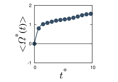
Figure 1: (Color online) The numerical verification of the inequality Eq. (17) for $t_{0}=0.0$. Here, $\left<\Omega^{*}(t)\right>=\left<\Omega(t)\right>_{\rm NE}/\sqrt{k/m}$ is plotted as a function of the scaled time $t*=t/\sqrt{m/k}$.

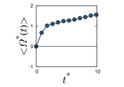
Figure 2: (Color online) The numerical verification of the inequality Eq. (17) for $t_{0}=1.0\sqrt{k/m}$. Here, $\left<\Omega^{*}(t)\right>=\left<\Omega(t)\right>_{\rm NE}/\sqrt{k/m}$ is plotted as a function of the scaled time $t*=t/\sqrt{m/k}$.

Figures 3 and 4 demonstrate that $\omega(t)$ introduced in Eq.(19) keeps to be zero within the numerical accuracy regardless of the choice of an initial condition, where Fig. 3 begins with an equilibrium condition ($t_{0}=0$), and Fig. 4 starts from a nonequilibrium condition ($t_{0}=1.0\sqrt{m/k})$. This result supports the validity of IFT (15) as well as its time differentiation Eq. (19). The results presented in Figs. 1-4 are remarkable, because, as stated previously, the higher order correlations produces $\omega(t)=0$, while $\omega(t)\simeq\left<\Omega(t)\right>$ is expected to be held under the decoupling approximation.

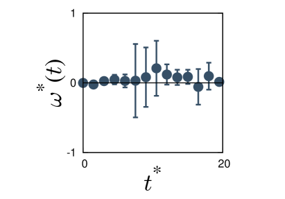
Figure 3: (Color online) The numerical verification of the integral fluctuation theorem Eq. (19) for $t_{0}=0.0$, where $\omega^{*}(t)=\omega(t)\sqrt{m/k}$ is plotted against the scaled time $t*=t\sqrt{k/m}$.

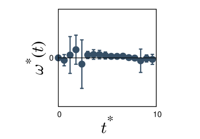
Figure 4: (Color online) The numerical verification of the integral fluctuation theorem Eq. (19) for $t_{0}=1.0\sqrt{m/k}$, where $\omega^{*}(t)=\omega(t)\sqrt{m/k}$ is plotted against the scaled time $t*=t\sqrt{k/m}$.

We note that IFT (15) contains all order of cumulants which is not suitable for numerical calculation. Nevertheless, such an identity is useful to test the validity of an approximate theory such as perturbation expansion.

IV.3 The verification of the generalized Green-Kubo formula

Let us verify the generalized Green-Kubo formula (28) in this subsection. Because we restrict our interest to the combination of steady processes as in Eq. (37), the generalized Green-Kubo formula (28) should be held. To verify the Green-Kubo formula we measure the average of the microscopic stress $\sigma_{xy}(t)$ in Eq. (39) . Figure 5 shows the results of two cases with $t_{0}=0$ and $t_{0}=5.0\sqrt{m/k}$, where we use $N=800,000$ independent samples. Although we have large fluctuations for the data with $t_{0}\neq 0$, we can conclude that the generalized Green-Kubo formula (28) is still valid even if we start from a nonequilibrium initial condition.

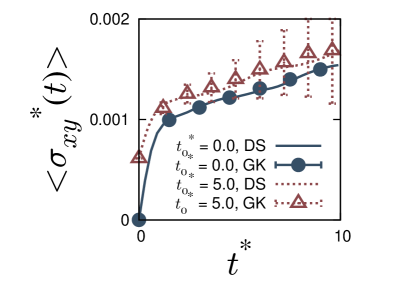
Figure 5: (Color online) The numerical verification of the generalized Green-Kubo formula in Eq.(28) for $t_{0}^{*}=t_{0}\sqrt{k/m}=0.0$ and $5.0$ through the plot of $\left<\sigma_{xy}^{*}(t)\right>=\left<\sigma_{xy}(t)\right>/(k/d)$ against the scaled time $t*=t\sqrt{k/m}$, where DS and GK, respectively, denote the numerical result in terms of the direct simulation of granular particles and the generalized Green-Kubo formula (28).

V Discussion

In this paper, we obtain some exact nonequilibrium relations, though the generalized Green-Kubo formula is only held for steady dynamics. To verify the validity, we have performed DEM of granular particles. We should stress that the identities presented in this paper can be used above the jamming transition.

Even after we confirm the validity of the nonequilibrium relations such as IFT and the generalized Green-Kubo formula, it is not easy to calculate the correlation function Eq. (28) analytically. One of possible methods is to use the mode-coupling theory (MCT). It is helpful to apply MCT for sheared liquids to characterize rheology near the jamming transition Suzuki-Hayakawa ; suzuki13 ; HO2008 ; miyazaki02 ; fuchs02 ; miyazaki04 ; fuchs05 ; fuchs09 . It is notable that Ref. Suzuki-Hayakawa develops a linear response theory for a sheared thermostat system around a nonequilibrium steady state. The application of this type of the response theory for granular fluids will be discussed elsewhere.

A different approach is to analyze the eigenvalue problem of the Liouville equation with the aid of full counting statistics sagawa2011 . This is also a promising approach, but the eigenvalue problem of the Liouville equation for granular liquids is not easy. We will also look for the possibility of this approach elsewhere.

We believe that Eq. (17) is the most important result in this paper, because this suggests that we may introduce the entropy-like quantity $S(\bm{\Gamma}(t))$ in Eq. (18) for an arbitrary dissipative system. In the standard statistical mechanics, the differentiation of the entropy with respect to the energy gives the inverse temperature. This idea still can be used for the statistical mechanics of granular gases.

For sheared and jammed granular systems under a constant volume condition, there are some papers to construct a statistical mechanics by using the stress ensemble henkes09 ; blumenfeld12 ; daniels13 ; max13 which might be the counter part of known Edwards ensemble Edwards89 for a system with a changing volume. Indeed, there are some advantages to use the stress $\Sigma_{xy}(\bm{\Gamma}(t))=V\sigma_{xy}(\bm{\Gamma}(t))$ for sheared and jammed granular systems, because the energy itself is small, and the stress should be spatially uniform in a steady state, while the energy is localized. Furthermore, we should indicate ${\rm Tr}\Sigma_{ij}$ is not far from the energy itself. Therefore, this paper may give some justification to introduce the effective temperature $T_{\rm eff}=\lim_{t\to\infty}(\partial S(\bm{\Gamma}(t))/\partial(\Sigma_{xy}(\bm{\Gamma}(t))\rangle_{\rm NE})^{-1}$ in the stress ensemble. The possibility to construct a statistical mechanics of granular systems which can cover granular gases, stress ensembles and the Edwards ensemble along this line will be discussed somewhere.

VI Summary

We obtained some exact relations for dissipative classical particles. We derived the integral fluctuation theorem (15) and its equivalent expression (19) around a nonequilibrium state, and confirmed the positivity of $\langle\Omega(\bm{\Gamma}(t))\rangle_{\rm NE}$ as in Eq. (17). From IFT we confirmed the existence of an entropy-like quantity (18) in an arbitrary dissipative system. We also derived the conventional fluctuation theorem (22). We gave a simple derivation of the Jarzynski equality (23). We also obtained the generalized Green-Kubo formula (28) for the steady dynamics around a nonequilibrium state. We numerically verified the validity of the obtained identities (19) and (28) as well as Eq. (17) for the case of sheared granular fluids.

Appendix A Alternative derivation of the integral fluctuation theorem

It is possible to obtain IFT from a different manner. Substituting Eq. (12) into Eq. (10) under the initial condition (14) for $t>0$ we obtain

$$\langle\check{A}(\bm{\Gamma}(-t))\rangle_{\rm NE}=\int d\mbox{\boldmath$\Gamma$}A(\mbox{\boldmath$\Gamma$})\tilde{U}_{\rightarrow}(0,t)\rho_{\rm NE}(\mbox{\boldmath$\Gamma$})$$ (43)

$$=\int d\mbox{\boldmath$\Gamma$}A(\mbox{\boldmath$\Gamma$})\left[e^{\int_{0}^{t}d\tau\Lambda(\bm{\Gamma}(\tau))}\rho_{\rm NE}(\mbox{\boldmath$\Gamma$}(t))\right].$$

Setting $\check{A}(\bm{\Gamma})=1$, the left hand side of Eq. (43) becomes one because of Eq. (10). On the other hand, if we adopt Eq. (14) with the aid of

$$\rho_{\rm NE}(\mbox{\boldmath$\Gamma$}(t))=e^{-I(\bm{\Gamma}(t))}/{\cal Z}=e^{-\int_{0}^{t}ds\dot{{I}}(\mathbf{\Gamma}(s))}\rho_{\rm NE}(\mbox{\boldmath$\Gamma$}),$$ (44)

we obtain IFT (15).

Appendix B Jarzynski equality of a gas starting from Eq.(20)

In this Appendix, we only focus on the Jarzynski equality of a gas starting from an equilibrium initial condition (20) to illustrate the meaning of the generalized Jarzynski equality introduced in Sec. III C. We also assume that the protocol parameter $\lambda(\tau)$ is proportional to the volume of system $V$. Here, we introduce the Hamiltonian $H_{\lambda}\equiv H(\bm{\Gamma}(\tau),\lambda(\tau))$ of the system for $0\leq\tau\leq t$.

Because the pressure $P$ is given by $P=-(\partial H_{\lambda}/\partial V)_{S}$ for an adiabatic process in thermodynamics, the work $W(t)$ acting on the system during the volume change $V(\lambda(\tau))$ for $0\leq\tau\leq t$ can be represented by $W(t)=\int_{0}^{t}d\tau\dot{V}(\partial H_{\lambda}/\partial V)_{S}=\int_{0}^{t}d\tau\dot{\lambda}(\partial H_{\lambda}/\partial\lambda)_{S}$, where $\dot{X}=dX(\tau)/d\tau$ for an arbitrary $X(\tau)$.

Now, let us discuss the change of the energy in the system

$$H(\bm{\Gamma}(t),1)-H(\bm{\Gamma}(0),0) = \int_{0}^{t}d\tau\frac{d}{d\tau}H(\bm{\Gamma}(\tau),\lambda(\tau))$$ (45)

$$= \int_{0}^{t}d\tau\Huge\{\dot{\lambda}(\tau)\frac{\partial H(\bm{\Gamma}(\tau),\lambda(\tau))}{\partial\lambda(\tau)}$$

$$+\dot{\bm{\Gamma}}(\tau)\cdot\frac{\partial H(\bm{\Gamma}(\tau),\lambda(\tau))}{\partial\bm{\Gamma}(\tau)}\Huge\}$$

$$= W(t)+Q(t),$$

where we have introduced the absorbing heat $Q(t)\equiv\int_{0}^{t}d\tau\dot{\bm{\Gamma}}(\tau)\cdot\frac{\partial H(\bm{\Gamma}(\tau),\lambda(\tau))}{\partial\bm{\Gamma}(\tau)}=\int_{0}^{t}d\tau i{\cal L}(\bm{\Gamma}(\tau))H_{\lambda}$ of the system. Note that $\dot{Q}(t)$ is given by $\dot{Q}(t)=-\beta V\sigma_{xy}(\bm{\Gamma}(t))-2\beta R(\bm{\Gamma}(t))$ for sheared granular systems introduced in Sec. IV.

Let us introduce the partition function $Z(\beta,t)\equiv\int d\bm{\Gamma}(t)e^{-\beta H(\bm{\Gamma}(t),\lambda(t)=1)}$ with the initial inverse temperature $\beta$. The change of $Z(\beta,t)$ is associated with the change of the free energy $\Delta F$ as

$$e^{-\beta\Delta F} = \frac{Z(\beta,t)}{Z(\beta,0)}=\frac{1}{Z(\beta,0)}\int d\bm{\Gamma}(t)e^{-\beta H(\bm{\Gamma}(t),1)}$$ (46)

$$= \int d\bm{\Gamma}\left|\frac{\partial\bm{\Gamma}(t)}{\partial\bm{\Gamma}}\right|\frac{e^{-\beta H(\bm{\Gamma},0)}}{Z(\beta,0)}e^{-\beta\int_{0}^{t}d\tau\frac{d}{d\tau}H(\bm{\Gamma}(\tau),\lambda(\tau))}$$

$$= \left\langle\exp\left[-\int_{0}^{t}d\tau\Omega_{\rm eq}(\bm{\Gamma}(\tau),\lambda(\tau))\right]\right\rangle_{\rm eq},$$

where $\Omega_{\rm eq}(\bm{\Gamma}(\tau),\lambda(\tau))=\beta\dot{W}(\tau)+\beta\dot{Q}(\tau)-\Lambda(\bm{\Gamma}(\tau))$. If the system dynamics is non dissipative, we have the relation $\dot{Q}(\tau)=\Lambda(\bm{\Gamma}(\tau))=0$, then the relation (46) is reduced to the conventional Jarzynski equality. For dissipative systems, it is reasonable that there exists a contribution from the effective absorbing heat $Q_{\rm eff}(t)=Q(t)-\beta^{-1}\int_{0}^{t}d\tau\Lambda(\bm{\Gamma}(\tau))=\beta^{-1}\int_{0}^{t}d\tau\Omega_{\rm eq}(\bm{\Gamma}(\tau),\lambda(\tau))$. In other words, the phase volume contraction is associated with the effective heat. This result is also reasonable, because the entropy production is given by $\int_{0}^{t}d\tau\Omega_{\rm eq}(\bm{\Gamma}(\tau),\lambda(\tau))$.

Appendix C Effect of measurement

Recently, Sagawa and Ueda sagawa have extended nonequilibrium identities to those under the effect of measurement. The effect of measurement appears through the mutual information

$${\cal I}[\mbox{\boldmath$\Gamma$}(t);y(t)]\equiv\ln\frac{P(y(t)|\mbox{\boldmath$\Gamma$}(t))}{P(y(t))},$$ (47)

where $y(t)$ represents a measurement outcome, and $P(y(t)|\mbox{\boldmath$\Gamma$}(t))$ is the conditional probability. The original formulation is applied to Hamilton dynamics, but it is easy to apply to the dissipative dynamics.

The generalized Jarzynski equality for sheared granular liquids is given by

$$\left\langle\left\langle\exp\left[-\int_{0}^{t}ds{\Omega}(\mathbf{\Gamma}(s))\right]e^{-{\cal I}(\bm{\Gamma})}e^{\Delta{\cal F}}\right\rangle\right\rangle=1,$$ (48)

where $\langle\langle A\rangle\rangle$ represents $\int d\mbox{\boldmath$\Gamma$}\prod_{t}dy(t)\frac{e^{-{\cal I}(\mathbf{\Gamma})}}{{\cal Z}(0)}P(y(t)|\mbox{\boldmath$\Gamma$}(t))A$ for any function $A$. Indeed, the left hand side of (48) is rewritten as

$${\rm LHS} = \int d\mbox{\boldmath$\Gamma$}\prod_{s}dy(s)\frac{e^{-I(\mathbf{\Gamma},0)}}{{\cal Z}(0)}P(y(s)|\mbox{\boldmath$\Gamma$}(s))$$ (49)

$$\times\exp\left[-\int_{0}^{t}ds\{\dot{I}(\mathbf{\Gamma}(s),\lambda(s))-\Lambda(\mathbf{\Gamma}(s))\}\right]$$

$$\times\frac{P(y(s))}{P(y(s)|\mbox{\boldmath$\Gamma$}(s))}\frac{{\cal Z}(0)}{{\cal Z}(t)},$$

where ${\cal Z}(t)=\int d\bm{\Gamma}e^{-I(\bm{\Gamma}(t),\lambda(t)=1)}$. This is reduced to 1 by using $\int d\mbox{\boldmath$\Gamma$}(t)=\int d\mbox{\boldmath$\Gamma$}e^{\int_{0}^{t}d\tau\Lambda(\mathbf{\Gamma}(\tau))}$.

References

• (1) D. N. Zubarev, Nonequilibrium Statistical Thermodynamics (Consultants Bureau, New York, 1974).
• (2) J. A. McLennan, Introduction to Nonequilibrium Statistical Mechanics (Prentice Hall, New Jersey, 1988).
• (3) D. J. Evans and G. P. Morriss, Statistical Mechanics of Nonequilibrium Liquids, 2nd ed. (Cambridge University Press, Cambridge, 2008).
• (4) G. P. Morriss and D. J. Evans, Phys. Rev. A 35, 792 (1987).
• (5) D. J. Evans, E. G. D. Cohen, and G. P. Morriss, Phys. Rev. Lett. 71, 2401 (1993).
• (6) G. Gallavotti and E. G. D. Cohen, Phys. Rev. Lett. 74, 2694 (1995).
• (7) C. Jarzynski, Phys. Rev. Lett. 78, 2690 (1997).
• (8) J. Kurchan, J. Phys. A: Math. Gen., 31, 3719 (1998).
• (9) G. E. Crooks, Phys. Rev. E 61, 2361 (2000).
• (10) T. Hatano and S. I. Sasa, Phys. Rev. Lett. 86, 3463 (2001).
• (11) D. J. Evans and D. J. Searles, Adv. Phys., 51, 1529 (2002).
• (12) U. Seifert, Rep. Prog. Phys. bf 75, 126001 (2012).
• (13) M. Esposito, U. Harbola, and S. Mukamel, Rev. Mod. Phys. 81, 1665 (2009).
• (14) J. Ren, P. Hänggi, and B. Li, Phys. Rev. Lett. 104, 170601 (2010).
• (15) K. Kanazawa, T. Sagawa, and H. Hayakawa, Phys. Rev. E 87, 052124 (2013).
• (16) K. Feitosa and N. Menon, Phys. Rev. Lett. 92, 164301 (2004).
• (17) N. Kumar, S. Ramaswamy, and A. K. Sood, Phys. Rev. Lett. 106, 118001 (2011).
• (18) S. Joubaud, D. Lohse, and D. van der Meer, Phys. Rev. Lett. 108, 210604 (2012).
• (19) A. Naert, EPL 97, 20010 (2012).
• (20) A. Mounier and A. Naert, EPL 100, 30002 (2012).
• (21) A. Puglisi, P. Visco, A. Barrat, E. Trizac, and F. van Wijland, Phys. Rev. Lett. 95, 110202 (2005).
• (22) A. Puglisi, P. Visco, E. Trizac, and F. van Wijland, EPL 72, 55 (2005).
• (23) A. Puglisi, P. Visco, E. Trizac, and F. van Wijland, Phys. Rev. E 73, 021301 (2006).
• (24) A. Puglisi, L. Rondoni, and A. Vulpiani, J. Stat. Mech. (2006) P08001.
• (25) A. Sarracino, D. Villamaina, G. Gradenigo, and A. Puglisi, EPL 92, 34001 (2010).
• (26) D. J. Evans and D. J. Searles, Phys. Rev. E 50, 1645 (1994).
• (27) U. Seifert, Phys. Rev. Lett. 95, 040602 (2005).
• (28) S.-H. Chong, M. Otsuki, and H. Hayakawa, Phys. Rev. E 81, 041130 (2010).
• (29) S.-H. Chong, M. Otsuki, and H. Hayakawa, Prog. Theor. Phys. Suppl. No.184, 77 (2010).
• (30) H. Hayakawa, S.-H. Chong, and M. Otsuki, in IUTAM-ISIMM Symposium on Mathematical Modeling and Physical Instances of Granular Flow, pp.19-30 edited by J. D. Goddard, J. T. Jenkins and P. Govine (AIP vol.1227, New York, 2010).
• (31) J. J. Brey, J. W. Dufty, and A. Santos, J. Stat. Phys. 87 (1997), 1051.
• (32) J. W. Dufty, A. Baskaran, and J. J. Brey, Phys. Rev. E 77, 031310 (2008).
• (33) A. Baskaran, J. W. Dufty ,and J. J. Brey, Phys. Rev. E 77, 031311 (2008).
• (34) H. Hayakawa and M. Otsuki, Prog. Theor. Phys. 119, 381 (2008).
• (35) S.-H. Chong, K. Suzuki, M. Otsuki, and H. Hayakawa, in preparation.
• (36) K. Suzuki and H. Hayakawa, Phys. Rev. E 87, 012304 (2013).
• (37) T. P. C. van Noije, M. H. Ernst, and R. Brito, Physica A 251, 266 (1998).
• (38) K. Kawasaki and J. D. Gunton, Phys. Rev. A 8, 2048 (1973).
• (39) D. J. Evans and G. P. Morriss, Statistical Mechanics of Nonequilibrium Liquids, 1st ed. (Academic Press, London, 1990).
• (40) K. Miyazaki and D. R. Reichman, Phys. Rev. E 66 (2002), 050501 (R).
• (41) M. Fuchs and M. E. Cates, Phys. Rev. Lett. 89, 248304 (2002).
• (42) K. Miyazaki, D. R. Reichman, and R. Yamamoto, Phys. Rev. E 70 (2004), 011501.
• (43) M. Fuchs and M. E. Cates, J. Phys.: Cond. Mat. 17 (2005), S1681.
• (44) M. Fuchs and M. E. Cates, J. Rheol. 53, 957 (2009).
• (45) K. Suzuki and H. Hayakawa, AIP Conf. Proc. 1542, 670 (2013).
• (46) T. Sagawa and H. Hayakawa, Phys. Rev. E 84, 051110 (2011).
• (47) S. Henkes and B. Chakraborty, Phys. Rev. E 79, 061301 (2009).
• (48) R. Blumenfeld, J. F. Jordan and S. F. Edwards, Phys. Rev. Lett. 109, 238001 (2012).
• (49) J. G. Puckett and K. E. Daniels, Phys. Rev. Lett. 110, 058001 (2013).
• (50) D. Bi, J. Zhang, R. P. Behringer and B. Chakraborty, EPL . 102, 34002 (2013).
• (51) S. F. Edwards and R. A. Oakeshot, Physica A 157, 1080- (1989).
• (52) T. Sagawa and M. Ueda, Phys. Rev. Lett. 104, 090602 (2010).