Closed form solution for the surface area, the capacitance and the demagnetizing factors of the ellipsoid

Abstract

We derive the closed form solutions for the surface area, the capacitance and the demagnetizing factors of the ellipsoid immersed in the Euclidean space $\mathbb{R}^{3}$. The exact solutions  for the above geometrical and physical properties of the ellipsoid are expressed  elegantly in terms of the generalized hypergeometric functions of Appell of two variables. Various limiting cases of the theorems of the exact solution for the surface area, the demagnetizing factors and the capacitance of the ellipsoid are derived, which agree with known solutions for the prolate and oblate spheroids and the sphere. Possible applications of the results achieved, in various fields of science, such as in physics, biology and space science are briefly discussed.

1 Introduction

An interesting and important problem of geometry and mathematical analysis is the exact answer to the question: which is the surface area of the ellipsoid immersed in the Euclidean space $\mathbb{R}^{3}$? Despite the simplicity of the question and the fact that the roots of the problem can be traced back to the 19th Century there has been only a partial progress towards its solution. This is because the closed form solution had evaded the efforts of previous researchers and scholars. The first serious investigation had been performed by Legendre who obtained an equation for the surface area of the ellipsoid in terms of formal integrals [1]. At this point we note, that a nice and critical review of the mathematical literature summarizing the attempts of various mathematicians in solving the problem, from the period of Legendre till 2005, has been written in [2] (see for instance [16]   cited in [2]). There is also a practical interest for an exact solution for the ellipsoidal surface area in various fields of science, we just mention a few such fields: 1) in biology the human cornea as well as the chicken erythrocytes are realistically described by an ellipsoid and the area is important in the latter case for the determination of the permeabilities of the cells [3],[4] 2) in cosmology and the physics of rotating black holes [5]and 3) in the geometry of hard ellipsoidal molecules and their virial coefficients. In particular in the latter case, the surface area appears in the expression for the pressure of the ellipsoidal molecules [6]. We also mention the relevance of the surface area of ellipsoid for the investigation and measurement of capillary forces between sediment particles and an air-water interface [7]. For an application to medicine we refer the reader to [8].

On the other hand there are two further important aspects related to the geometry of the ellipsoid awaiting for a full analytic solution with many important applications. Namely: first the calculation in closed analytic form of the capacitance of a conducting ellipsoid and second the exact analytic calculation of the demagnetizing factors of a magnetized ellipsoid.

In the former case, the geometry of the ellipsoid is complex enough to serve as a promising avenue for modeling arbitrarily shaped conducting bodies [9]. Capacitance modulation has been suggested recently as a method of detecting microorganisms such as the E. coli  present in the water [10]. Despite its importance in theory and applications, no exact analytic solution for the capacitance of the ellipsoid  had been derived by previous authors. There was only a formula in terms of formal integrals derived in [9].

In the later case, the magnetic susceptibility $\kappa$ of the body determined in the ambient magnetic field $\vec{B}$ is influenced by the shape and dimensions of the body. Thus the measured (apparent) magnetic susceptibility $\kappa_{A}$ should be corrected for this shape effect to obtain the shape-independent true susceptibility $\kappa_{T}.$ The relation between the true and apparent volume susceptibility involves the so called demagnetizing factors. The first attempts of calculating the demagnetizing factors  of the ellipsoid were made in [19],[20]. However, the authors of these works only derived expressions in terms of formal integrals.  In this paper, we derive for the first time the closed form solution for the three demagnetizing factors for the ellipsoid, in terms of the first hypergeometric function of Appell of two variables. A fundamental application of our work will be in the determination of asteroidal magnetic susceptibility and its comparison to those of meteorites in order to establish a meteorite-asteroid match [12]. Another interesting application of our solution for the demagnetizing factors of the ellipsoid would be in the field of microrobots. An external magnetic field can induce torque on a ferromagnetic body. Thus the use of external magnetic fields has strong advantages in microrobotics and biomedicine such as wireless controllability and safe use in clinical applications [11].

Thus, there is a certain demand from pure and applied mathematics for the closed form solutions of the above geometric problems. It is the purpose of our paper to produce such novel and useful exact analytic solutions for all three described problems above. We report our findings in what follows.

2 Closed form solution for the surface area of the ellipsoid.

We consider an ellipsoid centred at the coordinate origin, with rectangular Cartesian coordinate axes along the semi-axes $a,b,c:$

$$\frac{x^{2}}{a^{2}}+\frac{y^{2}}{b^{2}}+\frac{z^{2}}{c^{2}}=1.$$ (1)

We begin our exact analytic calculation for the infinitesimal surface area d$S,$ using the formula for the surface $\mathrm{Monge}$ segment :

$$\vec{x}(x,y)=(x,y,z(x,y)),$$ (2)

$$\mathrm{d}S=\left|\vec{x}_{x}\times\vec{x}_{y}\right|\mathrm{d}x\mathrm{d}y=\sqrt[2]{1+z_{x}^{2}+z_{y}^{2}}\mathrm{d}x\mathrm{d}y,$$ (3)

where $z_{x}:=\frac{\partial z(x.y)}{\partial x},$ $z_{y}:=\frac{\partial z(x,y)}{\partial y}$ and,

$$1+z_{x}^{2}+z_{y}^{2} =1+x^{2}\left(\frac{c^{2}}{a^{2}}\right)^{2}\frac{1}{c^{2}\left(1-\frac{x^{2}}{a^{2}}-\frac{y^{2}}{b^{2}}\right)}+y^{2}\left(\frac{c^{2}}{b^{2}}\right)^{2}\frac{1}{c^{2}\left(1-\frac{x^{2}}{a^{2}}-\frac{y^{2}}{b^{2}}\right)}$$

$$=1+x^{2}\left(\frac{c^{2}}{a^{4}}\right)\frac{1}{\left(1-\frac{x^{2}}{a^{2}}-\frac{y^{2}}{b^{2}}\right)}+y^{2}\left(\frac{c^{2}}{b^{4}}\right)\frac{1}{\left(1-\frac{x^{2}}{a^{2}}-\frac{y^{2}}{b^{2}}\right)}$$

$$=\frac{1-\frac{x^{2}}{a^{2}}-\frac{y^{2}}{b^{2}}+\frac{x^{2}c^{2}}{a^{4}}+\frac{y^{2}c^{2}}{b^{4}}}{1-\frac{x^{2}}{a^{2}}-\frac{y^{2}}{b^{2}}}=\frac{1-\left(1-\frac{c^{2}}{a^{2}}\right)\frac{x^{2}}{a^{2}}-\left(1-\frac{c^{2}}{b^{2}}\right)\frac{y^{2}}{b^{2}}}{1-\frac{x^{2}}{a^{2}}-\frac{y^{2}}{b^{2}}}\implies$$

Substituting to $(\ref{gensurfarea})$ we get

$$\mathrm{d}S =\sqrt[2]{\frac{1-\left(1-\frac{c^{2}}{a^{2}}\right)\frac{x^{2}}{a^{2}}-\left(1-\frac{c^{2}}{b^{2}}\right)\frac{y^{2}}{b^{2}}}{1-\frac{x^{2}}{a^{2}}-\frac{y^{2}}{b^{2}}}}\mathrm{d}x\mathrm{d}y$$

$$=\sqrt[2]{\frac{1-\delta\frac{x^{2}}{a^{2}}-\varepsilon\frac{y^{2}}{b^{2}}}{1-\frac{x^{2}}{a^{2}}-\frac{y^{2}}{b^{2}}}}\mathrm{d}x\mathrm{d}y,$$ (5)

where we define:

$$\delta:=1-c^{2}/a^{2},\text{ }\varepsilon:=1-c^{2}/b^{2}.$$ (6)

Consequently the octant surface area is given by$:$

$$\mathcal{A}_{oct.}^{ellipsoid} =\int_{0}^{a}\left\{\int_{0}^{b\sqrt[2]{1-x^{2}/a^{2}}}\sqrt[2]{\frac{1-\delta\frac{x^{2}}{a^{2}}-\varepsilon\frac{y^{2}}{b^{2}}}{1-\frac{x^{2}}{a^{2}}-\frac{y^{2}}{b^{2}}}}\mathrm{d}y\right\}\mathrm{d}x$$

$$=\int_{0}^{a}\left\{\int_{0}^{b\sqrt[2]{1-x^{2}/a^{2}}}\sqrt{\frac{\left(1-\delta\frac{x^{2}}{a^{2}}\right)\left[1-\frac{\varepsilon}{b^{2}\left(1-\delta\frac{x^{2}}{a^{2}}\right)}y^{2}\right]}{\left(1-\frac{x^{2}}{a^{2}}\right)\left[1-\frac{1}{b^{2}}\frac{1}{1-\frac{x^{2}}{a^{2}}}y^{2}\right]}}\mathrm{d}y\right\}\mathrm{d}x$$

$$=\int_{0}^{a}\left\{\int_{0}^{b\sqrt[2]{1-x^{2}/a^{2}}}\Omega\sqrt{\frac{(1-\mu^{2}y^{2})}{(1-\lambda^{2}y^{2}}}\mathrm{d}y\right\}\mathrm{d}x,$$ (7)

with

$$\Omega:=\sqrt[2]{\frac{\left(1-\delta\frac{x^{2}}{a^{2}}\right)}{\left(1-\frac{x^{2}}{a^{2}}\right)}},\text{ }\mu^{2}:=\frac{\varepsilon}{b^{2}(1-\delta x^{2}/a^{2})},\lambda^{2}:=\frac{1}{b^{2}}\frac{1}{1-\frac{x^{2}}{a^{2}}}.$$ (8)

We define a new variable:

$$y_{1}:=\frac{y}{b\sqrt[2]{1-x^{2}/a^{2}}}\implies\mathrm{d}y_{1}=\frac{\mathrm{d}y}{\eta},\text{ with }\eta:=b\sqrt[2]{1-x^{2}/a^{2}}.$$ (9)

Thus:

$$\mathcal{A}_{oct.}^{ellipsoid} =\int_{0}^{a}\left\{\int_{0}^{1}\Omega(x)\sqrt{\frac{1-\mu^{\prime 2}y_{1}^{2}}{1-\lambda^{\prime 2}y_{1}^{2}}}\mathrm{d}y_{1}\eta\right\}\mathrm{d}x$$

$$=\int_{0}^{a}\Omega(x)\eta(x)\left\{\int_{0}^{1}\sqrt{\frac{1-\mu^{\prime 2}\psi}{1-\lambda^{\prime 2}\psi}}\frac{\mathrm{d}\psi}{2\sqrt[2]{\psi}}\right\}\mathrm{d}x\implies$$ (10)

$$\mathcal{A}_{o\kappa\tau.}^{ellipsoid}=\int_{0}^{a}\Omega(x)\eta(x)\frac{1}{2}\frac{\Gamma(1/2)\Gamma(1)}{\Gamma(3/2)}F_{1}\left(\frac{1}{2},-\frac{1}{2},\frac{1}{2},\frac{3}{2},\mu^{\prime 2},\lambda^{\prime 2}\right){\rm d}x,$$ (11)

with

$$\mu^{\prime 2} :=\eta^{2}\mu^{2}=\frac{(1-x^{2}/a^{2})}{(1-\delta x^{2}/a^{2})}(1-c^{2}/b^{2}),$$ (12)

$$\lambda^{\prime 2} :=\eta^{2}\frac{1}{b^{2}(1-x^{2}/a^{2})}=\frac{b^{2}(1-x^{2}/a^{2})}{b^{2}(1-x^{2}/a^{2})}=1$$ (13)

and $F_{1}(\alpha,\beta,\beta^{\prime},\gamma,x,y)$ denotes the first generalized hypergeometric function of Appell [13] with two variables $x,y$ and parameters $\alpha,\beta,\beta^{\prime},\gamma:$

$$F_{1}(\alpha,\beta,\beta^{\prime},\gamma,x,y)=\sum_{m=0}^{\infty}\sum_{n=0}^{\infty}\frac{(\alpha,m+n)(\beta,m)(\beta^{\prime},n)}{(\gamma,m+n)(1,m)(1,n)}x^{m}y^{n}.$$ (14)

The double series converges absolutely for $|x|<1,|y|<1.$

Thus we obtain $:$

$$\mathcal{A}_{oct.}^{ellipsoid} =\int_{0}^{a}b\sqrt[2]{1-\frac{\delta x^{2}}{a^{2}}}\frac{1}{2}\frac{\Gamma(1/2)\Gamma(1)}{\Gamma(3/2)}F_{1}\left(\frac{1}{2},-\frac{1}{2},\frac{1}{2},\frac{3}{2},\mu^{\prime 2},1\right)\mathrm{d}x$$

$$=\int_{0}^{a}b\sqrt[2]{1-\frac{\delta x^{2}}{a^{2}}}\frac{1}{2}\frac{\Gamma(1/2)\Gamma(1)}{\Gamma(3/2)}\frac{\Gamma(3/2)\Gamma(1/2)}{\Gamma(1)\Gamma(1)}F\left(\frac{1}{2},-\frac{1}{2},1,\mu^{\prime 2}\right)\mathrm{d}x$$

$$=\int_{0}^{a}b\sqrt[2]{1-\frac{\delta x^{2}}{a^{2}}}\frac{\pi}{2}F\left(\frac{1}{2},-\frac{1}{2},1,\frac{(1-x^{2}/a^{2})}{(1-\delta x^{2}/a^{2})}(1-c^{2}/b^{2})\right)\mathrm{d}x.$$

In the transition from the first to the second line of the previous equation we made use of the property of Appell’s hypergeometric function according to which if one of its two variables is set to the value $1$ (one),  then the function $F_{1}$ reduces to the ordinary hypergeometric function of Gauß:

$$F_{1}\left(\frac{1}{2},-\frac{1}{2},\frac{1}{2},\frac{3}{2},\mu^{\prime 2},1\right)=\frac{\Gamma(3/2)\Gamma(3/2-1/2-1/2)}{\Gamma(3/2-1/2)\Gamma(3/2-1/2)}F\left(\frac{1}{2},-\frac{1}{2},\frac{3}{2}-\frac{1}{2},\mu^{\prime 2}\right).$$ (16)

It is also valid$:$

$$\mathcal{A}_{oct.}^{ellipsoid}=ab\int_{0}^{1}\sqrt[2]{1-\delta x_{1}^{2}}\frac{\pi}{2}F\left(\frac{1}{2},-\frac{1}{2},1,\frac{(1-x_{1}^{2})}{(1-\delta x_{1}^{2})}(1-c^{2}/b^{2})\right)\mathrm{d}x_{1}.$$ (17)

We now apply the transformation$:$

$$\frac{1-x_{1}^{2}}{1-\delta x_{1}^{2}}=1-\eta^{2}$$ (18)

which yields$:$

$$\mathcal{A}_{oct.}^{ellipsoid} =\frac{ab}{\sqrt[2]{1-\delta}}\int_{0}^{1}\frac{1}{\left[1+\frac{\delta\eta^{2}}{1-\delta}\right]^{2}}\frac{\pi}{2}F\left(\frac{1}{2},-\frac{1}{2},1,(1-\eta^{2})\varepsilon\right)\mathrm{d}\eta$$

$$=\frac{ab}{\sqrt[2]{1-\delta}}\int_{0}^{1}\sqrt[2]{1-\varepsilon\eta^{2}}\int_{0}^{\pi/2}\frac{1}{\left[1+\frac{\delta(1-\eta^{2})}{1-\delta}\cos^{2}\phi\right]^{2}}\mathrm{d}\phi\mathrm{d}\eta$$

$$=\frac{ab}{\sqrt[2]{1-\delta}}\int_{0}^{1}\sqrt[2]{1-\varepsilon\eta^{2}}\frac{\pi}{4}\frac{2+\frac{\delta(1-\eta^{2})}{1-\delta}}{\left[1+\frac{(\delta(1-\eta^{2}))}{1-\delta}\right]^{3/2}}\mathrm{d}\eta\implies$$ (19)

the total surface area is given by

$$\mathcal{A}^{ellipsoid} \mathcal{=}\frac{8ab}{\sqrt[2]{1-\delta}}\Biggl{\{}\int_{0}^{1}\sqrt[2]{1-\varepsilon\eta^{2}}\frac{\pi}{2}\frac{1}{\left\{1+\left[\frac{\delta(1-\eta^{2})}{1-\delta}\right]\right\}^{3/2}}\mathrm{d}\eta$$

$$+\int_{0}^{1}-\frac{\pi}{4}\frac{-\delta(1-\eta^{2})}{1-\delta}\frac{\sqrt[2]{1-\varepsilon\eta^{2}}}{\left\{1+\left[\frac{\delta(1-\eta^{2})}{1-\delta}\right]\right\}^{3/2}}\mathrm{d}\eta\Biggr{\}},$$ (20)

while using

$$1+\left[\frac{\delta(1-\eta^{2})}{1-\delta}\right]=\frac{1-\delta+\delta(1-\eta^{2})}{1-\delta}=\frac{1}{1-\delta}(1-\delta\eta^{2}),$$ (21)

we obtain$:$

$$\mathcal{A}^{ellipsoid} =\frac{8ab}{\sqrt[2]{1-\delta}}\Biggl{\{}\frac{\pi}{4}\frac{\Gamma(1/2)\Gamma(1)}{\Gamma(3/2)}\frac{1}{[1/(1-\delta)]^{3/2}}F_{1}\left(\frac{1}{2},\mathbf{\beta}_{\epsilon},\frac{3}{2},\varepsilon,\delta\right)$$

$$-\frac{\pi}{4}\frac{(-\delta)}{1-\delta}\frac{1}{[1/(1-\delta)]^{3/2}}\frac{1}{2}\frac{\Gamma(1/2)\Gamma(2)}{\Gamma(5/2)}F_{1}\left(\frac{1}{2},\mathbf{\beta}_{\epsilon},\frac{5}{2},\varepsilon,\delta\right)\Biggr{\}}$$

(22)

and we defined the 2-tuple:

$$\mathbf{\beta}_{\epsilon}:=\left(-\frac{1}{2},\frac{3}{2}\right).$$ (23)

Equation $(\ref{Area51eLL13KRANIOTIS})$ is our solution in closed analytic form for the surface area of the ellipsoid. We believe it constitutes the first complete exact analytic solution of the problem, while equation $(\ref{Area51eLL13KRANIOTIS})$ is of certain mathematical beauty. Thus, we have proved the theorem$:$

Theorem 1

The surface area of the general ellipsoid in closed analytic form is given by the equation$:$

$$\framebox{$\mathcal{A}_{scalene}^{ellipsoid}=\frac{8ab}{\sqrt[2]{1-\delta}}\Biggl{\{}\frac{\pi}{2}\frac{1}{[1/(1-\delta)]^{3/2}}F_{1}\left(\frac{1}{2},\mathbf{\beta}_{\epsilon},\frac{3}{2},\varepsilon,\delta\right)-\frac{\pi}{6}\frac{(-\delta)}{1-\delta}\frac{1}{[1/(1-\delta)]^{3/2}}F_{1}\left(\frac{1}{2},\mathbf{\beta}_{\epsilon},\frac{5}{2},\varepsilon,\delta\right)\Biggr{\}}$}\Longleftrightarrow$$

$$\framebox{$\mathcal{A}_{scalene}^{ellipsoid}=4\pi ab\left(\frac{c^{2}}{a^{2}}F_{1}(\frac{1}{2},-\frac{1}{2},\frac{3}{2},\frac{3}{2};\epsilon,\delta)+\frac{1}{3}\left(1-\frac{c^{2}}{a^{2}}\right)F_{1}(\frac{1}{2},-\frac{1}{2},\frac{3}{2},\frac{5}{2};\epsilon,\delta)\right)$}$$ (24)

The two-variables function $F_{1}\left(\alpha,\beta,\beta^{\prime},\gamma,x,y\right),$ admits the following integral representation which is of vital importance in the proof of the theorem eqn. $(\ref{Area51eLL13KRANIOTIS}),$ for the surface area of the general ellipsoid $:$

$${\displaystyle\int\limits_{0}^{1}}u^{\alpha-1}(1-u)^{\gamma-\alpha-1}(1-ux)^{-\beta}(1-uy)^{-\beta^{\prime}}du=\frac{\Gamma(\alpha)\Gamma(\gamma-\alpha)}{\Gamma(\gamma)}F_{1}\left(\alpha,\beta,\beta^{\prime},\gamma,x,y\right)\overset{}{}$$ (25)

We point out that in proving the theorem 1 we also produced the following interesting result:

Theorem 2

$$\int_{0}^{1}\sqrt[2]{1-\delta x_{1}^{2}}\frac{\pi}{2}F\left(\frac{1}{2},-\frac{1}{2},1,\frac{(1-x_{1}^{2})}{(1-\delta x_{1}^{2})}(1-c^{2}/b^{2})\right)\mathrm{d}x_{1}$$

$$=\frac{\pi}{2}(1-\delta)F_{1}\left(\frac{1}{2},\mathbf{\beta}_{\epsilon},\frac{3}{2},\varepsilon,\delta\right)+\frac{\pi}{6}\delta F_{1}\left(\frac{1}{2},\mathbf{\beta}_{\epsilon},\frac{5}{2},\varepsilon,\delta\right).$$ (26)

$\color[rgb]{0,0,1}Corollaries\;of\;Theorem\;\ref{GeorgiosVKraniotis}.$

A few special cases follow. In the case: $a=b\neq c$ the two variables of the hypergeometric function of Appell that appear in $(\ref{Area51eLL13KRANIOTIS})$ become equal and consequently $F_{1}$ reduces to the hypergeometric function of Gauß:

$$F_{1}\left(\frac{1}{2},-\frac{1}{2},\frac{3}{2},\frac{3}{2},1-\frac{c^{2}}{a^{2}},1-\frac{c^{2}}{a^{2}}\right)=F\left(\frac{1}{2},-\frac{1}{2}+\frac{3}{2},\frac{3}{2},1-\frac{c^{2}}{a^{2}}\right)$$ (27)

and $(\ref{Area51eLL13KRANIOTIS})$ takes the form$:$

$$\mathcal{A}_{a=b\neq c}^{\varepsilon\lambda\lambda\varepsilon\iota\psi o\varepsilon\iota\delta\acute{\epsilon}\varsigma} =\frac{8a^{2}}{\sqrt[2]{1-\delta}}\Biggl{\{}\frac{\pi}{4}2\frac{1}{[1/(1-\delta)]^{3/2}}F\left(\frac{1}{2},1,\frac{3}{2},1-\frac{c^{2}}{a^{2}}\right)$$

$$+-\frac{\pi}{4}\frac{(-\delta)}{1-\delta}\frac{1}{[1/(1-\delta)]^{3/2}}\frac{1}{2}\frac{4}{3}F\left(\frac{1}{2},1,\frac{5}{2},1-\frac{c^{2}}{a^{2}}\right)\Biggr{\}}$$

(28)

Equation $(\ref{OblateEllip})$ admits a further simplification$:$

Corollary 3

In the special case of an ellipsoid with $a=b>c$ ( oblate spheroid$)$ the following equation is valid$:$

$$\mathcal{A}_{a=b\neq c}^{\varepsilon\lambda\lambda\varepsilon\iota\psi o\varepsilon\iota\delta\acute{\epsilon}\varsigma} =\frac{8a^{2}}{\sqrt[2]{1-\delta}}\Biggl{\{}\frac{\pi}{4}2\frac{1}{[1/(1-\delta)]^{3/2}}F\left(\frac{1}{2},1,\frac{3}{2},1-\frac{c^{2}}{a^{2}}\right)$$

$$+-\frac{\pi}{4}\frac{(-\delta)}{1-\delta}\frac{1}{[1/(1-\delta)]^{3/2}}\frac{1}{2}\frac{4}{3}F\left(\frac{1}{2},1,\frac{5}{2},1-\frac{c^{2}}{a^{2}}\right)\Biggr{\}}$$

$$=2\pi a^{2}+\pi c^{2}\frac{1}{\sqrt[2]{1-c^{2}/a^{2}}}\log\frac{1+\sqrt[2]{1-c^{2}/a^{2}}}{1-\sqrt[2]{1-c^{2}/a^{2}}}.$$

Proof. We are going to make use of the formula [14] $:$

$$\log\frac{1+x}{1-x}=2xF\left(\frac{1}{2},1,\frac{3}{2},x^{2}\right),$$ (30)

and the contiguous equation:

$$F(\alpha,\beta,\gamma+1,z)=\frac{\gamma}{(\gamma-\alpha)(\gamma-\beta)}\left((1-z)\frac{\mathrm{d}}{\mathrm{d}z}+\gamma-\alpha-\beta\right)F(\alpha,\beta,\gamma,z).$$ (31)

Equation $(\ref{tomea1})$ yields$:$

$$\framebox{$F\left(\frac{1}{2},1,\frac{3}{2},1-\frac{c^{2}}{a^{2}}\right)=\frac{1}{2\text{ }\sqrt[2]{1-c^{2}/a^{2}}}\log\frac{1+\sqrt[2]{1-c^{2}/a^{2}}}{1-\sqrt[2]{1-c^{2}/a^{2}}},$}$$ (32)

while $(\ref{thome2})$

$$\framebox{$F\left(\frac{1}{2},1,\frac{5}{2},1-\frac{c^{2}}{a^{2}}\right)=\frac{3}{2}\left\{\frac{1}{1-c^{2}/a^{2}}-\frac{1}{2}\frac{c^{2}/a^{2}}{\left(1-\frac{c^{2}}{a^{2}}\right)^{3/2}}\log\frac{1+\sqrt[2]{1-c^{2}/a^{2}}}{1-\sqrt[2]{1-c^{2}/a^{2}}}\right\}.$}$$ (33)

Substituting equations $(\ref{GVKTOMAE}),(\ref{GVKTOM13})$ into $(\ref{OblateEllip})$ the corollary is proved.   

Corollary 4

In the special case of an ellipsoid with $a>b=c$ (prolate spheroid$)$ it holds$:$

$$\mathcal{A}_{a\neq b=c}^{ellipsoid} =\frac{8a^{2}}{\sqrt[2]{1-\delta}}\Biggl{\{}\frac{\pi}{4}2\frac{1}{[1/(1-\delta)]^{3/2}}F\left(\frac{1}{2},\frac{3}{2},\frac{3}{2},1-\frac{c^{2}}{a^{2}}\right)$$

$$+-\frac{\pi}{4}\frac{(-\delta)}{1-\delta}\frac{1}{[1/(1-\delta)]^{3/2}}\frac{1}{2}\frac{4}{3}F\left(\frac{1}{2},\frac{3}{2},\frac{5}{2},1-\frac{c^{2}}{a^{2}}\right)\Biggr{\}}$$

$$=2ab\pi\left(\sqrt[2]{\frac{b^{2}}{a^{2}}}+\frac{\sqrt[2]{(1-b^{2}/a^{2})}}{1-b^{2}/a^{2}}\arcsin\sqrt[2]{1-b^{2}/a^{2}}\right).$$

Proof. Indeed, for $b=c,$ the first variable of the Appell’s functions in the closed form solution of $(\ref{Area51eLL13KRANIOTIS})$ vanishes and the generalized hypergeometric functions in discussion reduce as follows$:$

$$F_{1}\left(\frac{1}{2},\mathbf{\beta}_{\varepsilon},\frac{3}{2},0,1-\frac{c^{2}}{a^{2}}\right) =F\left(\frac{1}{2},\frac{3}{2},\frac{3}{2},1-\frac{c^{2}}{a^{2}}\right),$$ (34)

$$F_{1}\left(\frac{1}{2},\mathbf{\beta}_{\varepsilon},\frac{5}{2},0,1-\frac{c^{2}}{a^{2}}\right) =F\left(\frac{1}{2},\frac{3}{2},\frac{5}{2},1-\frac{c^{2}}{a^{2}}\right)$$ (35)

We now apply the formulae $:$

$$F\left(\frac{1}{2},\frac{1}{2},\frac{3}{2},x\right)=\frac{1}{\sqrt[2]{x}}\arcsin\sqrt[2]{x},$$ (36)

$$F(\alpha,\beta+1,\gamma+1,x)-F(\alpha,\beta,\gamma,x) =\left(\frac{\gamma-\beta}{\beta\gamma}\right)x\frac{\mathrm{d}}{\mathrm{d}x}F(\alpha,\beta,\gamma+1,x),$$

$$F(\alpha,\beta+1,\gamma,x) =F(\alpha,\beta,\gamma,x)+\frac{x}{\beta}\frac{\mathrm{d}}{\mathrm{d}x}F(\alpha,\beta,\gamma,x).$$

We thus end up with the equations$:$

$$F\left(\frac{1}{2},\frac{3}{2},\frac{3}{2},x\right) =\frac{1}{\sqrt[2]{1-x}},$$ (39)

$$F\left(\frac{1}{2},\frac{3}{2},\frac{5}{2},x\right) =\frac{3}{2}\frac{\arcsin\sqrt[2]{x}}{x^{3/2}}-\frac{3}{2}\frac{\sqrt[2]{1-x}}{x},$$ (40)

and the corollary is proved.   

Corollary 5

In the special case of an ellipsoid with $a=c<b$ $($prolate spheroid$)$

$$\mathcal{A}_{a=c<b}^{ellipsoid} =\frac{8ab}{1}\frac{\pi}{2}F_{1}\left(\frac{1}{2},-\frac{1}{2},\frac{3}{2},\frac{3}{2},1-\frac{c^{2}}{b^{2}},0\right)$$

$$=4ab\pi F\left(\frac{1}{2},-\frac{1}{2},\frac{3}{2},1-\frac{c^{2}}{b^{2}}\right)$$

$$=2ab\pi\left\{\frac{c}{b}+\frac{\arcsin\sqrt[2]{1-c^{2}/b^{2}}}{\sqrt[2]{1-c^{2}/b^{2}}}\right\}.$$ (41)

Proof. Here we make use of the formulae$:$

$$F_{1}(\alpha,\beta,\beta^{\prime},\gamma,x,0)=F(\alpha,\beta,\gamma,x),$$ (42)

$$F(\alpha,\beta-1,\gamma,x)=\frac{1}{\gamma-\beta}\left[z(1-z)\frac{\mathrm{d}}{\mathrm{d}z}-\alpha z-\beta+\gamma\right]F(\alpha,\beta,\gamma,x)$$ (43)

and $(\ref{EIDIKOS}).$   

Corollary 6

In the particular case of the sphere $\ a=b=c$ $(\ref{Area51eLL13KRANIOTIS})$ reduces to the known result $\mathcal{A=}4\pi a^{2}.$

Let us give some examples of $(\ref{Area51eLL13KRANIOTIS}).$ For $a=2,b=1,c=0.25$ using $(\ref{Area51eLL13KRANIOTIS})$   we compute: $\mathcal{A}^{ellipsoid}=13.6992108087.$ For $a=1,b=1,c=0.5,$ we calculate $\mathcal{A}^{ellipsoid}=8.6718827033,$ and  for $a=1,b=0.8,c=0.625,$ we compute: $\mathcal{A}^{ellipsoid}=8.1516189229.$

3 Capacitance of a conducting ellipsoid.

For a conducting 3-dimensional ellipsoid $\mathbf{E}$ given by equation (1) its electrostatic capacitance is determined by solving Laplace’s equation:

$$\nabla^{2}\Phi=\frac{\partial^{2}\Phi}{\partial x^{2}}+\frac{\partial^{2}\Phi}{\partial y^{2}}+\frac{\partial^{2}\Phi}{\partial z^{2}}=0,$$ (44)

outside $\mathbf{E,}$ subject to $\Phi=1$ on the surface and $\Phi=0$ at $\infty$. The function $\Phi(\vec{x})$ is the (equilibrium) electrostatic potential of $\mathbf{E.}$

The computation is facilitated by ellipsoidal coordinates, a trick first introduced by Jacobi [15]. A point $\vec{x}$ outside $\mathbf{E}$ determines the parameter $0\leq r=r(\vec{x})<\infty$ by means of

$$\frac{x^{2}}{a^{2}+r}+\frac{y^{2}}{b^{2}+r}+\frac{z^{2}}{c^{2}+r}=1.$$ (45)

Now we look at:

$$\Phi(\vec{x})=\frac{1}{2}\int_{r(\vec{x})}^{\infty}\left[(a^{2}+r)(b^{2}+r)(c^{2}+r)\right]^{-1/2}\mathrm{d}r$$ (46)

outside $\mathbf{E.}$ It satisfies (44) and the prescribed conditions, therefore the capacitance is given by [17],[18]:

$$C^{-1}(\mathbf{E)=}\frac{1}{2}\int_{0}^{\infty}\frac{\mathrm{d}r}{\sqrt[2]{(a^{2}+r)(b^{2}+r)(c^{2}+r)}}$$ (47)

We will now show the following theorem in which we compute exactly the elliptic integral in $(\ref{ellipticinteC})$:

Theorem 7

The closed form solution for the capacitance of a 3-dimensional conducting ellipsoid is given by the expression:

$$C({\bf E})=\frac{2a\Gamma(3/2)}{\Gamma(1/2)\Gamma(1)}\frac{1}{F_{1}\left(\frac{1}{2},\frac{1}{2},\frac{1}{2},\frac{3}{2},x,y\right)},$$ (48)

where $x:=1-\frac{b^{2}}{a^{2}},y:=1-\frac{c^{2}}{a^{2}}$ and we organize the axes so that: $a>b>c>0.$

Equivalently, by substituting the values for the gamma function into $($48$)$: $\Gamma(3/2)=\frac{\sqrt[2]{\pi}}{2},$ $\Gamma(1/2)=\sqrt[2]{\pi},$ we derive:

$$C(\mathbf{E)=}\frac{a}{F_{1}\left(\frac{1}{2},\frac{1}{2},\frac{1}{2},\frac{3}{2},1-\frac{b^{2}}{a^{2}},1-\frac{c^{2}}{a^{2}}\right)}.$$ (49)

For the proof of theorem 7 see Appendix.

We also derive the following corollaries of Theorem 7:

Corollary 8

For the special case $a=b>c$ the capacitance of the spheroid is given by

$$C_{a=b>c}=\frac{2a\Gamma(3/2)}{\Gamma(1/2)}\frac{\sqrt[2]{1-c^{2}/a^{2}}}{\arcsin\sqrt[2]{1-c^{2}/a^{2}}}.$$ (50)

Proof. For $a=b>c,$ Eq. $(\ref{capacizeppelin})$ reduces to:

$$C =\frac{2a\Gamma(3/2)}{\Gamma(1/2)}\frac{1}{F_{1}(\frac{1}{2},\frac{1}{2},\frac{1}{2},\frac{3}{2},0,1-\frac{c^{2}}{a^{2}})}$$

$$=a\frac{1}{F\left(\frac{1}{2},\frac{1}{2},\frac{3}{2},1-\frac{c^{2}}{a^{2}}\right)}\overset{(\ref{EIDIKOS})}{=}a\frac{\sqrt[2]{1-c^{2}/a^{2}}}{\arcsin\sqrt[2]{1-c^{2}/a^{2}}}.$$ (51)

 

Corollary 9

For $b=c<a,$ the case of a prolate spheroid we derive

$$C_{b=c<a}=a\frac{2\sqrt[2]{1-c^{2}/a^{2}}}{\log\frac{1+\sqrt[2]{1-c^{2}/a^{2}}}{1-\sqrt[2]{1-c^{2}/a^{2}}}}$$ (52)

Proof. For $c=b<a,$ Eq. $(\ref{capacizeppelin})$ reduces to:

$$C =\frac{2a\Gamma(3/2)}{\Gamma(1/2)}\frac{1}{F_{1}\left(\frac{1}{2},\frac{1}{2},\frac{1}{2},\frac{3}{2},1-\frac{c^{2}}{a^{2}},1-\frac{c^{2}}{a^{2}}\right)}$$

$$=a\frac{1}{F\left(\frac{1}{2},1,\frac{3}{2},1-\frac{c^{2}}{a^{2}}\right)}\overset{(\ref{tomea1})}{=}a\frac{2\sqrt[2]{1-c^{2}/a^{2}}}{\log\frac{1+\sqrt[2]{1-c^{2}/a^{2}}}{1-\sqrt[2]{1-c^{2}/a^{2}}}}$$ (53)

 

Corollary 10

For a conducting sphere, $a=b=c,$ and equation $($48$)$ reduces to:

$$C_{sphere}=a.$$ (54)

Proof. For the case of the sphere the first hypergeometric function of Appell in $($48$)$ takes the value $1$.   

Corollary 11

For the case of an elliptic disk, $a>b>c=0,$ the capacitance is given in closed analytic form by:

$$C_{elliptic\text{ }disk}=\frac{a}{\frac{\pi}{2}F\left(\frac{1}{2},\frac{1}{2},1,1-\frac{b^{2}}{a^{2}}\right)}.$$ (55)

Proof. Indeed, in the case of an elliptic disk equation $($48$)$   reduces as follows:

$$C =\frac{a}{F_{1}\left(\frac{1}{2},\frac{1}{2},\frac{1}{2},\frac{3}{2},1-\frac{b^{2}}{a^{2}},1\right)}$$

$$=\frac{a}{\frac{\Gamma(3/2)\Gamma(3/2-1/2-1/2)}{\Gamma(3/2-1/2)\Gamma(3/2-1/2)}F\left(\frac{1}{2},\frac{1}{2},\frac{3}{2}-\frac{1}{2},1-\frac{b^{2}}{a^{2}}\right)}$$

$$=\frac{a}{\frac{\pi}{2}F\left(\frac{1}{2},\frac{1}{2},1,1-\frac{b^{2}}{a^{2}}\right)}$$ (56)

 

We now apply our closed form analytic solution $(\ref{capacizeppelin})$ for computing the capacitance of some ellipsoids. Our results are presented in Table 1.

$a=5,b=2,c=1$	$a=10,b=5,c=4$	$a=10,b=8,c=5$
$C/a=0.50822148949$	$C/a=0.621383016235$	$C/a=0.76121621804$

Table 1: Capacitance of some ellipsoids computed from (48)

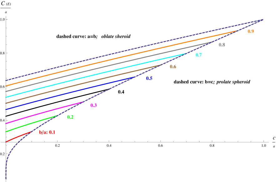
Figure 1: The capacitance $C(\mathbf{E})$ of a conducting ellipsoid immersed in $\mathbb{R}^{3}$ versus the ratio $c/a$ of the axes for various values of the ratio $b/a.$

In Figure 1 , we plot the capacitance $C(\mathbf{E})/a$ using Eqn.$(\ref{capacizeppelin}),$ of a conducting ellipsoid immersed in $\mathbb{R}^{3}$ versus the ratio $c/a$ of the axes for various values of the ratio $b/a.$

4 Demagnetizing factors of a magnetized ellipsoid

The first attempts of calculating the demagnetizing factors  of the ellipsoid were made in [19],[20]. However, the authors in [19],[20], only derived expressions in terms of formal integrals. We now derive the first closed form analytic solution  for the demagnetizing factors of the magnetized ellipsoid in terms of Appell’s first hypergeometric function $F_{1}$.

The potential in the interior of the magnetized ellipsoid is  a quadratic function of $x,y,$ and $z$ [19]:

$$\Phi_{int}=-Lx^{2}-My^{2}-Nz^{2}+W,$$ (57)

where the demagnetizing factors are defined by the integrals:

$$L =\pi a_{1}a_{2}a_{3}\kappa\int_{0}^{\infty}\frac{\mathrm{d}u}{(a_{1}^{2}+u)\sqrt{(a_{1}^{2}+u)(a_{2}^{2}+u)(a_{3}^{2}+u)}},$$ (58)

$$M =\pi a_{1}a_{2}a_{3}\kappa\int_{0}^{\infty}\frac{\mathrm{d}u}{(a_{2}^{2}+u)\sqrt{(a_{1}^{2}+u)(a_{2}^{2}+u)(a_{3}^{2}+u)}},$$ (59)

$$N =\pi a_{1}a_{2}a_{3}\kappa\int_{0}^{\infty}\frac{\mathrm{d}u}{(a_{3}^{2}+u)\sqrt{(a_{1}^{2}+u)(a_{2}^{2}+u)(a_{3}^{2}+u)}},$$ (60)

where we have the correspondence:

$$a_{1} =a,a_{2}=b,a_{3}=c,$$ (61)

$$a >b>c.$$ (62)

and

$$W=\pi a_{1}a_{2}a_{3}\kappa\int_{0}^{\infty}\frac{\mathrm{d}u}{\sqrt{(a_{1}^{2}+u)(a_{2}^{2}+u)(a_{3}^{2}+u)}}.$$ (63)

From Poisson’s differential equation

$$\nabla^{2}\Phi_{int}=-2(L+M+N)=-4\pi\kappa,$$ (64)

we derive the relationship that the demagnetizing factors satisfy:

$$L+M+N=2\pi\kappa.$$ (65)

Theorem 12

The closed form solution of the demagnetizing factors $L,M,N$, of the magnetized scalene ellipsoid is the following:

$$L =\frac{\pi abc}{a^{3}}\kappa\frac{\Gamma\left(\frac{3}{2}\right)\Gamma(1)}{\Gamma\left(\frac{5}{2}\right)}F_{1}\left(\frac{3}{2},\frac{1}{2},\frac{1}{2},\frac{5}{2},1-\frac{b^{2}}{a^{2}},1-\frac{c^{2}}{a^{2}}\right),$$ (66)

$$M =\frac{\pi abc}{a^{3}}\kappa\frac{\Gamma\left(\frac{3}{2}\right)\Gamma(1)}{\Gamma\left(\frac{5}{2}\right)}F_{1}\left(\frac{3}{2},\frac{3}{2},\frac{1}{2},\frac{5}{2},1-\frac{b^{2}}{a^{2}},1-\frac{c^{2}}{a^{2}}\right),$$ (67)

$$N =\frac{\pi abc}{a^{3}}\kappa\frac{\Gamma\left(\frac{3}{2}\right)\Gamma(1)}{\Gamma\left(\frac{5}{2}\right)}F_{1}\left(\frac{3}{2},\frac{1}{2},\frac{3}{2},\frac{5}{2},1-\frac{b^{2}}{a^{2}},1-\frac{c^{2}}{a^{2}}\right).$$ (68)

Proof. The demagnetizing factors are defined by the integrals eqns(58)-(60). We now compute these integrals in closed analytic form. We apply the transformation:

$$1+\frac{u}{a_{1}^{2}}=\frac{1}{x^{2}}\Rightarrow\mathrm{d}u=-\frac{2a_{1}^{2}}{x^{3}}\mathrm{d}x.$$ (69)

Consequently:

$$L=\frac{2\pi a_{1}a_{2}a_{3}\kappa}{a_{1}^{3}}\int_{0}^{1}\frac{\mathrm{d}x\text{ }x^{2}}{\sqrt[2]{(1-\mu_{2}x^{2})(1-\mu_{3}x^{2})}},$$ (70)

where we defined the moduli:

$$\mu_{2}:=1-\frac{a_{2}^{2}}{a_{1}^{2}},\text{ }\mu_{3}:=1-\frac{a_{3}^{2}}{a_{1}^{2}}.$$ (71)

We now set:

$$x^{2}=\xi\Rightarrow\mathrm{d}x=\frac{\mathrm{d}\xi}{2\sqrt[2]{\xi}}.$$ (72)

Thus

$$L =\frac{\pi a_{1}a_{2}a_{3}\kappa}{a_{1}^{3}}\int_{0}^{1}\frac{\mathrm{d}\xi\xi^{1/2}}{\sqrt[2]{(1-\mu_{2}\xi)(1-\mu_{3}\xi)}}$$

$$\overset{(\ref{INTREP})}{=}\frac{\pi abc\kappa}{a^{3}}\frac{\Gamma(3/2)\Gamma(1)}{\Gamma(5/2)}F_{1}\left(\frac{3}{2},\frac{1}{2},\frac{1}{2},\frac{5}{2},1-\frac{b^{2}}{a^{2}},1-\frac{c^{2}}{a^{2}}\right)$$ (73)

In a similar way, repeating the previous transformations, we compute analytically the two other demagnetizing factors $M,N.$ For instance:

$$N =\frac{\pi a_{1}a_{2}a_{3}\kappa}{a_{1}^{3}}\int_{0}^{1}\frac{\mathrm{d}\xi\xi^{1/2}}{(1-\mu_{3}\xi)\sqrt[2]{(1-\mu_{2}\xi)(1-\mu_{3}\xi)}}$$

$$=\frac{\pi bc\kappa}{a^{2}}\frac{\Gamma(3/2)\Gamma(1)}{\Gamma(5/2)}F_{1}\left(\frac{3}{2},\frac{1}{2},\frac{3}{2},\frac{5}{2},1-\frac{b^{2}}{a^{2}},1-\frac{c^{2}}{a^{2}}\right).$$ (74)

 

We now study special cases for the demagnetizing factors of the magnetized ellipsoid.

Corollary 13

In the special case $a=b>c$

$$L =\pi\frac{c}{a}\kappa\frac{\Gamma\left(\frac{3}{2}\right)\Gamma(1)}{\Gamma\left(\frac{5}{2}\right)}F_{1}\left(\frac{3}{2},\frac{1}{2},\frac{1}{2},\frac{5}{2},0,1-\frac{c^{2}}{a^{2}}\right)$$

$$=\pi\frac{c}{a}\kappa\frac{\Gamma\left(\frac{3}{2}\right)\Gamma(1)}{\Gamma\left(\frac{5}{2}\right)}F\left(\frac{3}{2},\frac{1}{2},\frac{5}{2},1-\frac{c^{2}}{a^{2}}\right)=\frac{\pi\kappa m^{2}}{(m^{2}-1)^{3/2}}\arcsin\frac{\sqrt[2]{m^{2}-1}}{m}-\frac{\pi\kappa}{m^{2}-1},$$

$$M =\pi\frac{c}{a}\kappa\frac{\Gamma\left(\frac{3}{2}\right)\Gamma(1)}{\Gamma\left(\frac{5}{2}\right)}F\left(\frac{3}{2},\frac{1}{2},\frac{5}{2},1-\frac{c^{2}}{a^{2}}\right)=\frac{\pi\kappa m^{2}}{(m^{2}-1)^{3/2}}\arcsin\frac{\sqrt[2]{m^{2}-1}}{m}-\frac{\pi\kappa}{m^{2}-1},$$

$$N =\pi\frac{c}{a}\kappa\frac{\Gamma\left(\frac{3}{2}\right)\Gamma(1)}{\Gamma\left(\frac{5}{2}\right)}F_{1}\left(\frac{3}{2},\frac{1}{2},\frac{3}{2},\frac{5}{2},0,1-\frac{c^{2}}{a^{2}}\right)$$

$$=\pi\frac{c}{a}\kappa\frac{\Gamma\left(\frac{3}{2}\right)\Gamma(1)}{\Gamma\left(\frac{5}{2}\right)}F\left(\frac{3}{2},\frac{3}{2},\frac{5}{2},1-\frac{c^{2}}{a^{2}}\right)=\frac{2\pi\kappa m^{2}}{m^{2}-1}\left\{\frac{-\arcsin\frac{\sqrt[2]{m^{2}-1}}{m}}{\sqrt[2]{m^{2}-1}}+1\right\}$$ (77)

where $m:=a/c.$

Proof. For $a=b>c,$

$$L=M=\pi\frac{c}{a}\kappa\frac{\Gamma\left(\frac{3}{2}\right)\Gamma(1)}{\Gamma\left(\frac{5}{2}\right)}F\left(\frac{3}{2},\frac{1}{2},\frac{5}{2},1-\frac{c^{2}}{a^{2}}\right).$$ (78)

Using the contiguous relations

$$z\frac{\mathrm{d}}{\mathrm{d}z}F(\alpha,\beta,\gamma,z) =\alpha\left[F(\alpha+1,\beta,\gamma,z)-F(\alpha,\beta,\gamma,z)\right],$$ (79)

and Eq.(31)

$$\frac{1}{2}F\left(\frac{3}{2},\frac{1}{2},\frac{5}{2},\overset{:=z}{\overbrace{1-\frac{c^{2}}{a^{2}}}}\right)=\frac{1}{2}F\left(\frac{1}{2},\frac{1}{2},\frac{5}{2},z\right)+z\frac{\mathrm{d}}{\mathrm{d}z}F\left(\frac{1}{2},\frac{1}{2},\frac{5}{2},z\right),$$ (80)

with

$$F\left(\frac{1}{2},\frac{1}{2},\frac{5}{2},z\right)=\frac{3}{2}\left[(1-z)\left\{-\frac{1}{2z^{3/2}}\arcsin\sqrt[2]{z}+\frac{1}{2z}\frac{1}{\sqrt[2]{1-z}}\right\}+\frac{1}{2}\frac{\arcsin\sqrt[2]{z}}{\sqrt[2]{z}}\right].$$ (81)

Consequently:

$$L=M=\frac{\pi\kappa m^{2}}{(m^{2}-1)^{3/2}}\arcsin\frac{\sqrt[2]{m^{2}-1}}{m}-\frac{\pi\kappa}{m^{2}-1},$$ (82)

where $z=1-\frac{c^{2}}{a^{2}}:=1-\frac{1}{m^{2}}$. On the other hand, using the contiguous relation (79) for the calculation of the $N$-demagnetizing factor, yields:

$$z\frac{\mathrm{d}}{\mathrm{d}z}F(\alpha,\beta,\gamma,z) =\alpha\left[F(\alpha+1,\beta,\gamma,z)-F(\alpha,\beta,\gamma,z)\right]\Rightarrow$$ (83)

$$\frac{1}{2}F\left(\frac{3}{2},\frac{3}{2},\frac{5}{2},z\right) =\frac{1}{2}F\left(\frac{1}{2},\frac{3}{2},\frac{5}{2},z\right)+z\frac{\mathrm{d}}{\mathrm{d}z}F\left(\frac{1}{2},\frac{3}{2},\frac{5}{2},z\right),$$ (84)

where the Gauß function $F\left(\frac{1}{2},\frac{3}{2},\frac{5}{2},z\right)$ is given by Equation (40). Consequently,

$$\frac{1}{2}F\left(\frac{3}{2},\frac{3}{2},\frac{5}{2},z\right)=-\frac{6}{4}\frac{\arcsin\sqrt[2]{z}}{z^{3/2}}+\frac{3}{4}\frac{\sqrt[2]{1-z}}{z}+\frac{3}{4}\frac{1}{\sqrt[2]{1-z}}\left(\frac{1}{z}+1\right),$$ (85)

and $N$ is given by Equation (77).   

Corollary 14

In the special case $b=c<a$

$$L =\frac{\pi c^{2}}{a^{2}}\frac{\kappa\Gamma\left(\frac{3}{2}\right)\Gamma(1)}{\Gamma\left(\frac{5}{2}\right)}F\left(\frac{3}{2},1,\frac{5}{2},1-\frac{c^{2}}{a^{2}}\right)$$

$$=\frac{2\pi\kappa}{m^{2}-1}\left\{\frac{m}{2}\log\frac{m+\sqrt[2]{m^{2}-1}}{m-\sqrt[2]{m^{2}-1}}-1\right\},m:=a/c,$$ (86)

$$N =\frac{\pi c^{2}}{a^{2}}\frac{\kappa\Gamma\left(\frac{3}{2}\right)\Gamma(1)}{\Gamma\left(\frac{5}{2}\right)}F\left(\frac{3}{2},2,\frac{5}{2},1-\frac{c^{2}}{a^{2}}\right)$$

$$=\kappa\pi\frac{m}{m^{2}-1}\left[-\frac{1}{2}\frac{1}{\sqrt[2]{m^{2}-1}}\log\frac{m+\sqrt[2]{m^{2}-1}}{m-\sqrt[2]{m^{2}-1}}+m\right]$$ (87)

Proof. For $b=c<a$

$$N =\frac{\pi ac^{2}}{a^{3}}\kappa\frac{\Gamma\left(\frac{3}{2}\right)\Gamma(1)}{\Gamma\left(\frac{5}{2}\right)}F_{1}\left(\frac{3}{2},\frac{1}{2},\frac{3}{2},\frac{5}{2},1-\frac{c^{2}}{a^{2}},1-\frac{c^{2}}{a^{2}}\right)$$

$$=\frac{\pi ac^{2}}{a^{3}}\kappa\frac{\Gamma\left(\frac{3}{2}\right)\Gamma(1)}{\Gamma\left(\frac{5}{2}\right)}F\left(\frac{3}{2},2,\frac{5}{2},\overset{z:=}{\overbrace{1-\frac{c^{2}}{a^{2}}}}\right)=\frac{\pi c^{2}}{a^{2}}\frac{\kappa\Gamma\left(\frac{3}{2}\right)\Gamma(1)}{\Gamma\left(\frac{5}{2}\right)}3\frac{\mathrm{d}}{\mathrm{d}z}F\left(\frac{1}{2},1,\frac{3}{2},z\right)$$

$$\overset{(\ref{tomea1})}{=}\frac{\pi c^{2}}{a^{2}}\frac{\kappa\Gamma\left(\frac{3}{2}\right)\Gamma(1)}{\Gamma\left(\frac{5}{2}\right)}\frac{3}{2}\left\{-\frac{1}{2}\frac{1}{z^{3/2}}\log\frac{1+\sqrt[2]{z}}{1-\sqrt[2]{z}}+\frac{1}{z(1-z)}\right\}$$

$$\overset{z=1-1/m^{2}}{=}\kappa\pi\frac{m}{m^{2}-1}\left[-\frac{1}{2}\frac{1}{\sqrt[2]{m^{2}-1}}\log\frac{m+\sqrt[2]{m^{2}-1}}{m-\sqrt[2]{m^{2}-1}}+m\right]$$ (88)

 

Corollary 15

For a magnetized sphere, $a=b=c,$ and the demagnezing factors are all equal to:

$$L=M=N=\frac{2\pi\kappa}{3}.$$ (89)

Proof. In this case, the generalized hypergeometric functions of Appell that appear in the exact solutions for the demagnetizing factors, eqns$(\ref{magnitisena})-(\ref{magnitis3}),$ take the value $1.$   

We now apply our closed form analytic solutions for the demagnetizing factors, Eqns. $(\ref{magnitisena})-(\ref{magnitis3}),$ in order to compute these factors for various ellipsoids.  Our results are summarized in Tables 2 $,\ref{GVKGOSBORN}$.

$a=3,b=2,c=1$	$a=4,b=3,c=2$	$a=10,b=3,c=2$
$\frac{L}{4\pi}=0.156300698829271$	$\frac{L}{4\pi}=0.211265605319304$	$\frac{L}{4\pi}=0.0725156494555862$
$\frac{M}{4\pi}=0.267154040262005$	$\frac{M}{4\pi}=0.305006257867421$	$\frac{M}{4\pi}=0.366221770806668$
$\frac{N}{4\pi}=0.576545260908724$	$\frac{N}{4\pi}=0.483728136813275$	$\frac{N}{4\pi}=0.561262579737746$

Table 2: The demagnetizing factors $L/4\pi,M/4\pi,N/4\pi$ as computed from the equations of Theorem 12, for various ellipsoids.

	$\frac{c}{a}$	$\frac{b}{a}$	$\frac{L}{4\pi}$	$\frac{M}{4\pi}$	$\frac{N}{4\pi}$
1.$\begin{array}[c]{c}\text{Theorem \ref{magnetization} }\\ \text{Numerical Osborn}\end{array}$	$0.017452$	$0.99620$	$\begin{array}[c]{c}0.0133953\\ \end{array}$	$\begin{array}[c]{c}0.0134714\\ 0.013471\end{array}$	$\begin{array}[c]{c}0.973133\\ \end{array}$
2.$\begin{array}[c]{c}\text{Theorem \ref{magnetization} }\\ \text{Numerical Osborn}\end{array}$	$0.087156$	$0.984920$	$\begin{array}[c]{c}0.0613072\\ 0.06108\end{array}$	$\begin{array}[c]{c}0.062672\\ 0.06281\end{array}$	$\begin{array}[c]{c}0.876021\\ 0.87611\end{array}$
3.$\begin{array}[c]{c}\text{Theorem \ref{magnetization} }\\ \text{Numerical Osborn}\end{array}$	$0.5$	$0.98863$	$\begin{array}[c]{c}0.235445\\ 0.23555\end{array}$	$\begin{array}[c]{c}0.238955\\ 0.23885\end{array}$	$\begin{array}[c]{c}0.5256\\ 0.5256\end{array}$
4.$\begin{array}[c]{c}\text{Theorem \ref{magnetization} }\\ \text{Numerical Osborn}\end{array}$	$0.087156$	$1$	$\begin{array}[c]{c}0.0615658\\ 0.06154\end{array}$	$\begin{array}[c]{c}0.0615658\\ 0.06154\end{array}$	$\begin{array}[c]{c}0.876868\\ 0.87692\end{array}$

Table 3: The demagnetizing factors for various values of the ratios $c/a,b/a$ and a comparison with the numerical results of reference [20]. Empty entries in the table means that the author of [20] did not provide such values.

We also plot the demagnetizing factors $L/4\pi,M/4\pi,N/4\pi$ of the magnetized ellipsoid versus the ratio $c/a,$ for various values of the ratio $b/a.$ Our results are displayed in Figures 2,3,4.

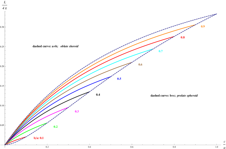
Figure 2: The $L-$ demagnetizing factor versus the ratio $c/a$ for various values of the ratio $b/a.$

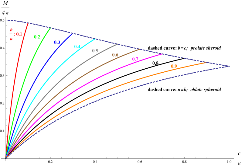
Figure 3: The $M-$demagnetizing factor versus the ratio $c/a$ for various values of the ratio $b/a.$ The dashed curves meet at the point determined in Corollary 15.

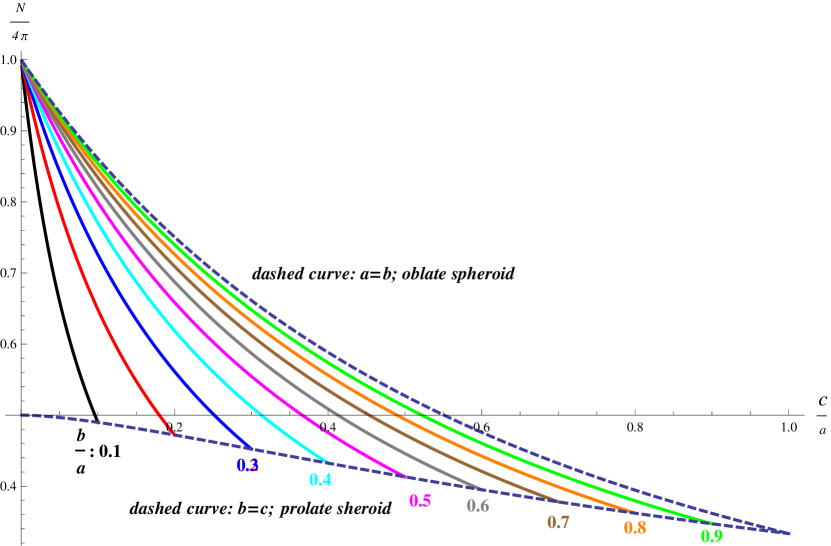
Figure 4: The $N$ demagnetizing factor versus the ratio $c/a$ for various values of the ratio $b/a.$

Using theorem 12 we can write for the potential $\Phi_{int}:$

$$\Phi_{int}=\mathcal{A}\left\{1-\left(\frac{x^{2}}{\alpha^{2}}+\frac{y^{2}}{\beta^{2}}+\frac{z^{2}}{\gamma^{2}}\right)\right\},$$ (90)

where

$$\alpha :=3\frac{F_{1}\left(\frac{1}{2},\frac{1}{2},\frac{1}{2},\frac{3}{2},1-\frac{b^{2}}{a^{2}},1-\frac{c^{2}}{a^{2}}\right)}{F_{1}\left(\frac{3}{2},\frac{1}{2},\frac{1}{2},\frac{5}{2},1-\frac{b^{2}}{a^{2}},1-\frac{c^{2}}{a^{2}}\right)}a^{2},$$ (91)

$$\beta :=3\frac{F_{1}\left(\frac{1}{2},\frac{1}{2},\frac{1}{2},\frac{3}{2},1-\frac{b^{2}}{a^{2}},1-\frac{c^{2}}{a^{2}}\right)}{F_{1}\left(\frac{3}{2},\frac{3}{2},\frac{1}{2},\frac{5}{2},1-\frac{b^{2}}{a^{2}},1-\frac{c^{2}}{a^{2}}\right)}b^{2},$$ (92)

$$\gamma :=3\frac{F_{1}\left(\frac{1}{2},\frac{1}{2},\frac{1}{2},\frac{3}{2},1-\frac{b^{2}}{a^{2}},1-\frac{c^{2}}{a^{2}}\right)}{F_{1}\left(\frac{3}{2},\frac{1}{2},\frac{3}{2},\frac{5}{2},1-\frac{b^{2}}{a^{2}},1-\frac{c^{2}}{a^{2}}\right)}c^{2},$$ (93)

$$\mathcal{A} :=2\kappa\pi\frac{b}{a}\frac{c}{a}a^{2}F_{1}\left(\frac{1}{2},\frac{1}{2},\frac{1}{2},\frac{3}{2},1-\frac{b^{2}}{a^{2}},1-\frac{c^{2}}{a^{2}}\right).$$ (94)

5
Concluding remarks

We have solved analytically a number of problems related to the geometrical and physical properties of the theory of ellipsoid.

In particular, we have solved in closed analytic form for the capacitance of a conducting ellipsoid immersed in the Euclidean space $\mathbb{R}^{3}.$ The exact solution has been expressed in terms of Appell’s first hypergeometric function $F_{1}$ and it is given by Theorem 7 and equation  $(\ref{CapaciGVKellipsoid}).$ We have also computed exactly the capacitance of a conducting ellipsoid in $n-$dimensions. The resulting exact analytic solution is expressed in terms of Lauricella’s fourth hypergeometric function $F_{D}$ of $n-1$-variables, see Theorem 16, equation $(\ref{GVKcapacityND}).$

We subsequently solved analytically for the demagnetizing factors of a magnetized ellipsoid immersed in the Euclidean space $\mathbb{R}^{3}.$ The resulting solutions are expressed elegantly in terms of Appell’s first hypergeometric function $F_{1},$ as stated in Theorem 12 and equations $(\ref{magnitisena})-(\ref{magnitis3}).$

Finally, we have derived the closed form solution for the geometrical entity of the surface area of the ellipsoid immersed in the Euclidean space $\mathbb{R}^{3}.$ Our analytic solution in this case is given in Theorem 1, eqn.$(\ref{Area51eLL13KRANIOTIS}).$

We believe that the useful exact analytic theory of the ellipsoid we have developed in this work will have many applications in various scientific fields. We have already outlined in the introduction possible multidisciplinary applications of our theory in science; a scientific multidisciplinarity which measures from physics, biology  and chemistry to micromechanics, space science and astrobiology.

A fundamental mathematical generalization of our theory would be to investigate the immersion of an ellipsoid in curved spaces and solve for the corresponding geometrical and physical properties of such an object. However, such a project is beyond the scope of the present paper and it will be a subject of a future publication.

Appendix A Appendix

The generalization of Theorem 7 for the capacitance of the ellipsoid in $n$-dimensions involves the analytic computation of a hyperelliptic integral. Hyperelliptic integrals which are involved in the solution of timelike and null geodesics in Kerr and Kerr-(anti) de Sitter black hole spacetimes have been computed analytically in references [21],[22], in terms of the multivariable Lauricella’s hypergeometric function $F_{D}$. The idea is to bring a hyperelliptic integral by the appropriate transformations onto the integral representation that the function $F_{D}$ admits .

Applying this method for the analytic computation of the capacitance of the ellipsoid in $n$-dimensions, generalizes Theorem 7 to the following one:

Theorem 16

The closed form solution for the capacitance of a $n-$dimensional conducting ellipsoid is given by the formula:

$$C=\frac{2a_{1}^{n-2}\Gamma\left(\frac{n}{2}\right)}{\Gamma\left(\frac{n-2}{2}\right)\Gamma(1)}\frac{1}{F_{D}\left(\frac{n-2}{2},\underset{n-1}{\underbrace{\frac{1}{2},\frac{1}{2},\ldots,\frac{1}{2}}},\frac{n}{2},x_{2},x_{3},\ldots,x_{n}\right)}$$ (95)

where $F_{D}$ denotes the fourth hypergeometric function of Lauricella of $n-1$-variables and

$$x_{2}:=1-\frac{a_{2}^{2}}{a_{1}^{2}},x_{3}:=1-\frac{a_{3}^{2}}{a_{1}^{2}},\ldots,x_{n}:=1-\frac{a_{n}^{2}}{a_{1}^{2}}.$$ (96)

Proof. Applying the transformation (69) to the hyperelliptic integral

$$\frac{1}{C}=\frac{1}{2}\int_{0}^{\infty}\frac{\mathrm{d}u}{\sqrt{(a_{1}^{2}+u)(a_{2}^{2}+u)\cdots(a_{n}^{2}+u)}},$$ (97)

yields:

$$\frac{1}{C} =\frac{1}{a_{1}^{n-2}}\int_{0}^{1}\frac{x^{n-3}\mathrm{d}x}{\sqrt[2]{(1-\mu_{2}x^{2})(1-\mu_{3}x^{2})\cdots(1-\mu_{n}x^{2})}}$$

$$\overset{x^{2}=\xi}{=}\frac{1}{2a_{1}^{n-2}}\int_{0}^{1}\frac{\xi^{\frac{n-3-1}{2}}\mathrm{d}\xi}{\sqrt[2]{(1-\mu_{2}\xi)(1-\mu_{3}\xi)\cdots(1-\mu_{n}\xi)}}$$

$$=\frac{1}{2a_{1}^{n-2}}\frac{\Gamma\left(\frac{n-2}{2}\right)\Gamma(1)}{\Gamma\left(\frac{n}{2}\right)}F_{D}\left(\frac{n-2}{2},\underset{n-1}{\underbrace{\frac{1}{2},\frac{1}{2},\ldots,\frac{1}{2}}},\frac{n}{2},x_{2},x_{3},\ldots,x_{n}\right)$$ (98)

where

$$\mu_{j}\equiv x_{j}:=1-\frac{a_{j}^{2}}{a_{1}^{2}},j=1,2,\ldots,n,$$ (99)

and

$$a_{1}\geq a_{2}\geq\ldots\geq a_{n}>0$$ (100)

For $n=3$ we derive

$$\frac{1}{C}=\frac{1}{2a_{1}}\frac{\Gamma(1/2)\Gamma(1)}{\Gamma(3/2)}F_{1}\left(\frac{1}{2},\frac{1}{2},\frac{1}{2},\frac{3}{2},1-\frac{b^{2}}{a^{2}},1-\frac{c^{2}}{a^{2}}\right),$$ (101)

and thus Theorem 7 is proved as well.   

Applying our closed form analytic formula, eqn.(95), for $n=4,$ and the choice of values $a_{1}=2,a_{2}=1+2/3,a_{2}=1+1/3,a_{4}=1$ we derive for the capacitance of this particular higher dimensional ellipsoid:

$$C_{(n=4)}=4.406592791665676649174487.$$ (102)

The generalization of Theorem 12 in $n$-dimensions is the following:

Theorem 17

$$\mathcal{L}^{(n)} =\frac{\pi a_{1}a_{2}a_{3}\ldots a_{n}}{a_{1}^{n}}\frac{\Gamma\left(\frac{n}{2}\right)\Gamma(1)}{\Gamma\left(\frac{n+2}{2}\right)}F_{D}\left(\frac{n}{2},\underset{n-1}{\underbrace{\frac{1}{2},\frac{1}{2},\ldots,\frac{1}{2}}},\frac{n+2}{2},\mu_{2},\ldots,\mu_{n}\right),$$

$$\mathcal{M}^{(n)} =\frac{\pi a_{1}a_{2}a_{3}\ldots a_{n}}{a_{1}^{n}}\frac{\Gamma\left(\frac{n}{2}\right)\Gamma(1)}{\Gamma\left(\frac{n+2}{2}\right)}F_{D}\left(\frac{n}{2},\frac{3}{2},\frac{1}{2},\ldots,\frac{1}{2},\frac{n+2}{2},\mu_{2},\ldots,\mu_{n}\right),$$

The fourth hypergeometric function of Lauricella $F_{D}$ of $m$-variables [24] is defined as follows:

$$\framebox{$\displaystyle F_{D}(\alpha,\mbox{\boldmath${\beta}$},\gamma,{\bf z})\equiv F_{D}^{(m)}(\alpha,\mbox{\boldmath${\beta}$},\gamma,{\bf z}):=\sum_{n_{1},n_{2},\dots,n_{m}=0}^{\infty}\frac{(\alpha)_{n_{1}+\cdots n_{m}}(\beta_{1})_{n_{1}}\cdots(\beta_{m})_{n_{m}}}{(\gamma)_{n_{1}+\cdots+n_{m}}(1)_{n_{1}}\cdots(1)_{n_{m}}}z_{1}^{n_{1}}\cdots z_{m}^{n_{m}}$}$$ (105)

where

$$\mathbf{z} = (z_{1},\ldots,z_{m}),$$

$${\beta} = (\beta_{1},\ldots,\beta_{m}).$$ (106)

The Pochhammer symbol $\displaystyle(\alpha)_{m}=(\alpha,m)$ is defined by

$$(\alpha)_{m}=\frac{\Gamma(\alpha+m)}{\Gamma(\alpha)}=\left\{\begin{array}[]{ccc}1,&{\rm if}&m=0\\ \alpha(\alpha+1)\cdots(\alpha+m-1)&\text{{\rm if}}&m=1,2,3\end{array}\right.$$ (107)

The series admits the following integral representation:

$$\framebox{$\displaystyle F_{D}(\alpha,\mbox{\boldmath${\beta}$},\gamma,{\bf z})=\frac{\Gamma(\gamma)}{\Gamma(\alpha)\Gamma(\gamma-\alpha)}\int_{0}^{1}t^{\alpha-1}(1-t)^{\gamma-\alpha-1}(1-z_{1}t)^{-\beta_{1}}\cdots(1-z_{m}t)^{-\beta_{m}}{\rm d}t$}$$ (108)

which is valid for $\displaystyle{\rm Re}(\alpha)>0,\;{\rm Re}(\gamma-\alpha)>0.$. It converges absolutely inside the $m$-dimensional cuboid

$$|z_{j}|<1,(j=1,\ldots,m).$$ (109)

It also has the following values:

$$F_{D}^{(n)}(\alpha,\beta_{1},\ldots,\beta_{n},\gamma,1,x_{2},\ldots,x_{n})$$

$$=\frac{\Gamma(\gamma)\Gamma(\gamma-\alpha-\beta_{1})}{\Gamma(\gamma-\alpha)\Gamma(\gamma-\beta_{1})}F_{D}^{(n-1)}(\alpha,\beta_{2},\ldots,\beta_{n},\gamma-\beta_{1},x_{2},\ldots,x_{n}),$$ (110)

when $\max\{|x_{2}|,\ldots,|x_{n}|\}<1,$ $\operatorname{Re}(\gamma-\alpha-\beta_{1})>0.$

References

[1]A.M. Legendre,“Exercises de
Calcul Intégral”, (Huzard-Coursier, Paris, 1811) 182-194.
[2]G. J. Tee, “Surface area of ellipsoid
segment”, Technical report; Department of Mathematics,
University of Auckland, New Zeland
[3]L. S. Kwok, “Calculation and
Application of the Anterior Surface Area of a Model Human Cornea”, J. Theor.Biol. (1984), 295-313
[4]B. T. Bulliman and P. W. Kuchel, “A
series Expression for the Surface Area of an Ellipsoid and its Application to
the Computation of the Surface Area of Avian Eythrocytes”,
J. Theor. Biol. (1988) 134, 113-123
[5]A. Krasiński, “Ellipsoidal
Space-Times, Sources for the Kerr Metric”, Annals of
Physics, 112, (1978) 22-40
[6]G. S. Singh and B. Kumar, “Geometry of
hard ellipsoidal fluids and their virial coefficients”, J.
Chem.Phys. 105, (1996), 2429-2435
[7]N. Chatterjee et al, “Capillary Forces between Sediment Particles and an Air-Water
Interface”, Environ. Sci. Technol. (2012) 46, 4411-4418
[8]D. Xu, et al,“The ellipsoidal
area ratio: an alternative anisotropy index for diffusion tensor
imaging”, Magn. Reson. Imaging, (2009) 27, 311-323
[9]T. H. Shumpert, “Capacitance
Calculations for Satellites, Part I. Isolated Capacitances of Ellipsoidal
Shapes with comparisons to Some other Simple Bodies”, Sensor
and Simulation Notes, Note 157, 1972, 1-30
[10]A. Kumar et al, “Detection
of E.coli Cell using Capacitance Modulation”, Proceedings of
the COMSOL Conference 2010, India
[11]Soichiro Tottori et al, “Selective control method for multiple magnetic helical microrobots”, J. Micro-Nano Mech. (2011) 6, 89-95
[12]T. Kohut et al, “Physical
properties of meteorites-Applications in space missions to asteroids”, Meteoritics & Planetary Science 43, 6, (2008) 1009-1020
[13]Appell P 1882 Sur les fonctions
hypergéométriques de deux variables J. Math. Pures Appl. Liouville 8 173–216
[14]L. W. Thomé, “Über die
Kettenbruchentwickelung der Gausschen Function F(a,1,y,x)”Journal für die reine und angewandte Mathematik, (Crelle’s
Journal), , 322-336.
[15]C. G. J. Jacobi, “Vorlesungen
über Dynamik”, 1866
[16]S. R. Keller, “On the Surface Area of
the Ellipsoid”, Mathematics of Computation, (1979),
33, 310-314; L. R.M. Maas, “On the surface
area of an ellipsoid and related integrals of elliptic integrals”, Journal of Computational and applied mathematics 51 (1994) 237-249
[17]G. J. Tee, “Surface area and Capacity
of Ellipsoids in n Dimensions” Technical report; Department
of Mathematics, University of Auckland, New Zeland, 2003-3-16
[18]G. Pólya and G. Szegö, “Inequalities for the capacity of a condenser” Americal Journal of Mathematics, Vol. 67 (1945), pp 1-32
[19]O. Kellogg, “Foundations of
Potential Theory”, Springer, Berlin (1929)
[20]J. A. Osborn, “Demagnetizing factors
of the General Ellipsoid”, Phys.Rev. 67, (1945), 351-357
[21]G. V. Kraniotis, “Frame
dragging and bending of light in Kerr and Kerr-(anti) de Sitter spacetimes”, Class. Quantum Grav. 22 (2005) 4391-4424; G. V. Kraniotis,
“Periapsis and gravitomagnetic precessions of stellar
orbits in Kerr and Kerr-de Sitter black hole spacetimes”,
Class. Quantum Grav. 24 (2007) 1775-1808
[22]G. V. Kraniotis, “Precise
analytic treatment of Kerr and Kerr-(anti) de Sitter black holes as
gravitational lenses”, Class. Quantum Grav. 28 (2011) 085021
[23]G. M. Scarpello, D. Ritelli, “The
hyperelliptic integrals and ” , Journal of Number
Theory 129 (2009) 3094-3108
[24]G. Lauricella, “Sulle funzioni
ipergeometriche a piu variabili”, Rend.Circ.Mat.Palermo 7
(1893), 111-158
[25]J. Zsigrai, “Ellipsoidal shapes in
general relativity: general definitions and an application”,
Class. Quantum Grav. 20 (2003), 2855-2870