Scaling between magnetic and lattice fluctuations in iron-pnictide superconductors

Abstract

The phase diagram of the iron arsenides is dominated by a magnetic and a structural phase transition, which need to be suppressed in order for superconductivity to appear. The proximity between the two transition temperature lines indicates correlation between these two phases, whose nature remains unsettled. Here, we find a scaling relation between nuclear magnetic resonance (NMR) and shear modulus data in the tetragonal phase of electron-doped $\mathrm{Ba(Fe_{1-x}Co_{x})_{2}As_{2}}$ compounds. Because the former probes the strength of magnetic fluctuations while the latter is sensitive to orthorhombic fluctuations, our results provide strong evidence for a magnetically-driven structural transition.

The fact that superconductivity in most iron arsenide materials appears in close proximity to a magnetic phase transition reviews led to the early proposal that magnetic fluctuations play a fundamental role in promoting Cooper pairing reviews_pairing . Indeed, the NMR spin-lattice relaxation rate $1/T_{1}$, which is proportional to the strength of spin fluctuations, is substantially enhanced in optimally doped compounds, where the superconducting transition temperature $T_{c}$ acquires its highest value, and rather small in strongly overdoped samples, where $T_{c}$ vanishes Ning10 . At the same time, a tetragonal-to-orthorhombic phase transition is always found near the magnetic transition, and, consequently, in the vicinity of the superconducting dome Fisher11 ; Fisher12 . Measurements of the shear elastic modulus $C_{s}$, which is the inverse susceptibility of the orthorhombic distortion, also found a clear correlation between the strength of lattice fluctuations and $T_{c}$ FernandesPRL10 ; Yoshizawa12 ; Bohmer . Therefore, the road towards the understanding of the high-temperature superconducting state in the iron pnictides necessarily passes through the understanding of the relationship between the magnetic and structural transitions.

That these two phases are correlated is evident from the phase diagram of the iron pnictides, since the structural transition line (at temperature $T_{s}$) and the magnetic transition line (at temperature $T_{N}\leq T_{s}$) follow each other closely in the normal state as doping (or pressure) is changed Nandi10 ; Kim11 ; Birgeneau11 (see Fig. 3). Although strong evidence has been given for an electronic mechanism driving the structural transition Fisher12 , the key unresolved issue is its microscopic nature. Two competing approaches have been proposed, where magnetic fluctuations play a fundamentally distinct role. One point of view is based on strong inter-orbital interactions that lead to orbital order and may induce magnetism as a secondary effect w_ku10 ; Phillips10 ; devereaux10 ; Phillips12 ; Stanev13 . Alternatively, spin fluctuations are considered the driving force behind the structural transition by inducing strong nematic Xu08 ; Fang08 ; Fernandes12 ; Indranil11 or closely related orbital fluctuations Kontani12 ; Kontani_solidstate . While it is clear that both degrees of freedom are important to correctly describe the electronic orthorhombic phase SUST12 ; Dagotto13 , it is crucial to establish which of the two is the primary one, since both orbital KontaniPRB12 ; Ono10 and spin fluctuations reviews_pairing have been proposed as candidates for the unconventional pairing state of the pnictides.

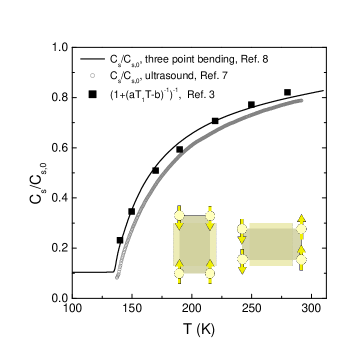
Figure 1: Scaling between the shear modulus $C_{s}$ (open symbols, from Ref. Yoshizawa12 , continuous line from Ref. Bohmer ) and the NMR spin-lattice relaxation rate $1/T_{1}$ (closed symbols, from Ref. Ning10 ) in the tetragonal phase of the parent compound $\mathrm{BaFe_{2}As_{2}}$. $C_{s,0}$ denotes the non-critical, high-temperature shear modulus. The fitting parameters are $a=0.65$ (sK)^-1 and $b=1.3$ in Eq. (2). The inset schematically represents the magneto-elastic coupling, which makes bonds connecting anti-parallel (parallel) spins expand (shrink).

Differentiating between the two proposed scenarios is difficult in the symmetry-broken state, because all possible order parameters are non-zero at $T<T_{s}$: orthorhombicity, orbital polarization, magnetic anisotropy, etc Davis10 ; Duzsa11 ; Uchida11 ; ZXshen11 ; Greene12 ; Matsuda12 ; Imai12 . Instead, additional information can be obtained by studying the fluctuations associated with each degree of freedom in the tetragonal phase at $T>T_{s}$ Gallais13 . In this regime, it holds generally that the electronic driven softening of the elastic shear modulus $C_{s}$ is determined by the static susceptibility $\chi_{\mathrm{nem}}\equiv\left\langle\varphi\varphi\right\rangle$ associated with the electronic degree of freedom $\varphi$ that drives the structural transition:

$$\frac{C_{s}}{C_{s,0}}=\left(1+\frac{\lambda^{2}}{C_{s,0}}\chi_{\mathrm{nem}}\right)^{-1}$$ (1)

The tetragonal symmetry is broken once $\left\langle\varphi\right\rangle\neq 0$, which gives rise to a finite orthorhombic distortion $\epsilon_{xx}-\epsilon_{yy}\propto\left\langle\varphi\right\rangle$. In the orbital fluctuations model, $\varphi$ corresponds to the difference between the occupations of the $d_{xz}$ and $d_{yz}$ orbitals, and $\lambda$ is the coupling between the lattice and orbital distortions Phillips10 . On the other hand, in the spin-nematic case, $\varphi$ is an Ising-type degree of freedom referring to the relative orientation of neighboring spin polarizations and $\lambda$ is the magneto-elastic coupling FernandesPRL10 . $C_{s,0}$ is the bare shear modulus in the absence of these electronic degrees of freedoms.

In this paper, we show that the nematic susceptibility $\chi_{\mathrm{nem}}$ is closely related to the dynamic spin susceptibility, strongly supporting a magnetically-driven structural transition in the $\mathrm{Ba(Fe_{1-x}Co_{x})_{2}As_{2}}$ family of pnictides. Specifically, we show that spin fluctuations, given by the NMR spin-lattice relaxation rate $1/T_{1}$, and orthorhombic fluctuations, given by the shear modulus $C_{s}$, satisfy the scaling relation:

$$\frac{C_{s}}{C_{s,0}}=\frac{1}{1+\left[a\left(T_{1}T\right)-b\right]^{-1}}$$ (2)

with doping-dependent, but temperature-independent constants $a$ and $b$. The spin-lattice relaxation rate and the shear modulus data considered here are the ones previously presented in Refs. Ning10 and Bohmer , respectively. The raw data contains contributions from critical fluctuations - which is our interest here - and non-critical processes, which are unrelated to the magnetic or structural transitions. To make a meaningful scaling analysis, we need to disentangle these two contributions. The NMR $1/T_{1}T$ is given by:

$$\frac{1}{T_{1}T}=\gamma_{g}^{2}\lim_{\omega\rightarrow 0}\sum_{\mathbf{k}}F^{2}\left(\mathbf{k}\right)\frac{\mathrm{Im}\,\chi\left(\mathbf{k},\omega\right)}{\omega}$$ (3)

where $\chi\left(\mathbf{k},\omega\right)$ denotes the dynamic magnetic susceptibility at momentum $\mathbf{k}$ and frequency $\omega$. Here, $\gamma_{g}$ is the constant gyromagnetic ratio and $F\left(\mathbf{k}\right)$ is the structure factor of the hyperfine interaction, which depends on the direction of the applied field. The critical magnetic fluctuations are associated with the ordering vectors $\mathbf{Q}_{1}=\left(\pi,0\right)$ or $\mathbf{Q}_{2}=\left(0,\pi\right)$ of the magnetic striped state, and lead to the divergence of $1/T_{1}T$ as the temperature is lowered towards the magnetic transition. By choosing the applied magnetic field parallel to the FeAs plane, the structure factor $F\left(\mathbf{k}\right)$ is enhanced at the ordering vector $\mathbf{Q}$, favoring the dominant contribution of the critical fluctuations Shannon11 . To remove the non-critical Korringa contribution coming from small momenta $\mathbf{k}\approx 0$, we follow Ref. Ning10 and subtract from $1/T_{1}T$ the data of a heavily overdoped composition ($x=0.14$) which is sufficiently far from magnetic and structural instabilities. This is justified in this family of compounds due to the nearly doping-independent shape of the Knight shift, which may be different in other series NMR_Oka ; NMR_Nakai ; NMR_Hirano . We note, however, that our scaling analysis is robust and holds even for other choices of background subtraction.

Similarly, strongly overdoped samples display a rather different temperature dependence for the shear modulus than underdoped and optimally doped samples. While in the latter a critical softening of the shear modulus is observed as the temperature decreases, in the former $C_{s}$ hardens slightly at low temperatures because of phonon anharmonicity. Thus, to obtain the critical contribution to the shear modulus, we used the data of a heavily overdoped sample ($x=0.33$) as background, as explained in Bohmer .

Figure 1 presents both the shear modulus data of Ref. Bohmer (continuous curve) and the rescaled spin-lattice relaxation rate (3) of Ref. Ning10 (closed symbols) for the undoped ($x=0$) composition. The agreement is excellent for the entire temperature range, providing strong support for the existence of a true scaling between spin and lattice fluctuations. Interestingly, recent Raman scattering measurements in the tetragonal phase of the same compound found that the orbital fluctuations are not strong enough to account for the experimentally observed softening of the shear modulus Gallais13 . For completeness, we also display in Fig. 1 the shear modulus data of Ref. Yoshizawa12 (open symbols), to show the agreement between the ultrasound technique of the latter work and the three-point bending method of Ref. Bohmer . We note that the differences in the two sets of data arise mostly from disparities in the transition temperatures associated with sample preparation.

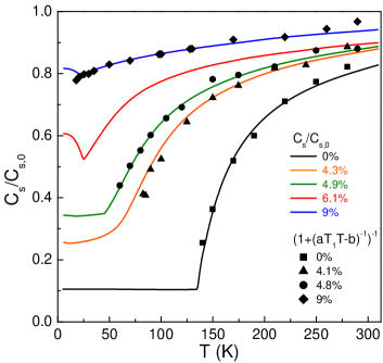
Figure 2: Comparison between the relative shear modulus $C_{s}/C_{s,0}$ (continuous lines, from Ref. Bohmer ) and the rescaled NMR $1/T_{1}T$ (closed symbols, from Ref. Ning10 ) for different “effective” Co concentrations in $\mathrm{Ba(Fe_{1-x}Co_{x})_{2}As_{2}}$. The “effective” Co concentration was determined by comparing the available transition temperatures ($T_{s}$, $T_{N}$, $T_{c}$) of the two sets of samples with a third independent phase diagram (from Ref.Chu09 ).

To show that this agreement is not fortuitous, we also analyzed doped samples, see Fig. 2. In this case, the comparison is complicated by the fact that the two groups in Refs. Ning10 and Bohmer did not use the same samples and the determination of the Co content may differ. For this reason, we determine an “effective” Co-content by comparing the available transition temperatures ($T_{s}$, $T_{N}$, $T_{c}$) of the two sets of samples with a third independent phase diagram (from Ref. Chu09 ). The values are indicated in Fig. 2 and differ only slightly from those given in the respective references.

Our analysis of the rescaled $T_{1}T$ data presented in Fig. 2 remarkably captures the doping evolution of the temperature-dependent shear modulus. The doping dependence of the scaling parameters $a$ and $b$ is shown in Fig. 3. While $a$ is roughly constant across the entire phase diagram, $b$ is significantly suppressed, approaching zero near optimal doping. Note from Eq. (2) that $b$ is not a Curie-Weiss temperature, but a parameter that measures the separation between the magnetic and structural instabilities. Thus, its vanishing suggests that the two instabilities tend to the same temperature. We will come back to this point below.

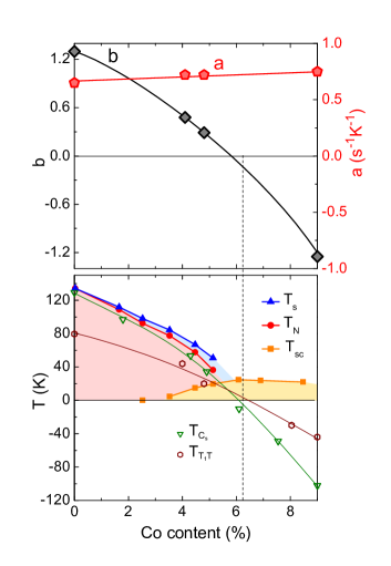
Figure 3: Doping dependence of the fitting parameters $a$ and $b$, and the phase diagram of $\mathrm{Ba(Fe_{1-x}Co_{x})_{2}As_{2}}$. Notice that $a$ remains nearly constant, whereas $b$ aproaches zero near optimal doping, where the superconducting transition temperature is the highest. The transition temperatures in the phase diagram were obtained from resistivity measurements of Ref. Chu09 . The bare transition temperatures $T_{T1T}$ and $T_{C_{s}}$ are obtained from Curie-Weiss fittings of the data from Ref. Ning10 and Bohmer , respectively. Lines are a guides to the eye.

Having established experimentally the existence of the scaling relation (2), we now discuss its origin using a general magneto-elastic model FernandesPRL10 ; Cano10 ; Qi09 ; Gorkov09 ; Indranil11 . Since we removed the non-critical contributions to $1/T_{1}T$ and $C_{s}$, a low-energy model suffices. In particular, we consider two magnetic order parameters $\mathbf{M}_{1}$ and $\mathbf{M}_{2}$, referring to the magnetic striped states with ordering vectors $\mathbf{Q}_{1}=\left(\pi,0\right)$ (i.e. spins parallel along $\hat{\mathbf{y}}$ and anti-parallel along $\hat{\mathbf{x}}$) and $\mathbf{Q}_{2}=\left(0,\pi\right)$ (i.e. spins parallel along $\hat{\mathbf{x}}$ and anti-parallel along $\hat{\mathbf{y}}$) Fernandes12 . We also include the orthorhombic order parameter $\delta=\epsilon_{xx}-\epsilon_{yy}$, where $\epsilon_{ij}\equiv\frac{1}{2}\left(\partial_{i}u_{j}+\partial_{j}u_{i}\right)$ is the strain tensor. For simplicity, we consider here the coordinate system referring to the 1-Fe unit cell. The action of the collective magnetic degrees of freedom is given by:

$$S_{\mathrm{mag}}= \sum_{q,i}\chi^{-1}\left(q\right)\mathbf{M}_{i,q}\cdot\mathbf{M}_{i,-q}+\frac{u}{2}\sum_{r}\left(M_{1}^{2}+M_{2}^{2}\right)^{2}$$

$$-\frac{g_{0}}{2}\sum_{r}\left(M_{1}^{2}-M_{2}^{2}\right)^{2}$$ (4)

where $u,g_{0}>0$ are constants and we introduced the notations $q=\left(\mathbf{q},\omega\rightarrow i\omega_{n}-i0^{+}\right)$ and $r=\left(\mathbf{r},\tau\right)$, with $\tau$ denoting imaginary time and $\omega_{n}=2n\pi T$, Matsubara frequency. At the mean-field level, minimization of this free energy leads to the two magnetic stripe configurations when $\chi^{-1}\left(\mathbf{Q}\right)\rightarrow 0$, i.e. we obtain either $M_{1}=0$, $M_{2}\neq 0$ or $M_{1}\neq 0$, $M_{2}=0$. This free energy can in fact be microscopically derived from models of either itinerant electrons Fernandes12 ; Brydon11 ; Haas13 or localized spins Fang08 ; batista .

The lattice contribution to the action is given by:

$$S_{\mathrm{el}}=\sum_{r}\left[\frac{1}{2}C_{s,0}\delta^{2}-\lambda\delta\left(M_{1}^{2}-M_{2}^{2}\right)\right]$$ (5)

The first term is just the harmonic part of the elastic energy, while the second one is the magneto-elastic coupling, with arbitrary coupling constant $\lambda>0$. This coupling makes bonds connecting anti-parallel (parallel) spins expand (shrink) in the orthorhombic phase (see inset of Fig. 1). In principle, one could assume that $C_{s,0}$ itself becomes zero at a certain temperature. Here, instead, we assume $C_{s,0}$ to be constant and to never become soft on its own. Then we can integrate out the Gaussian orthorhombic fluctuations and derive the shear modulus $C_{s}$ renormalized by spin fluctuations, obtaining $\chi_{\mathrm{nem}}$ of Eq.1 as $\chi_{\mathrm{nem}}^{-1}=\chi_{0,\mathrm{nem}}^{-1}-g$. The bare nematic susceptibility is determined by the dynamic spin-susceptibility $\chi\left(q\right)$ properly renormalized by magnetic fluctuations, $\chi_{0,\mathrm{nem}}=\sum\limits_{q}\chi^{2}\left(q\right)$. The nematic coupling $g$ is the bare coupling $g_{0}$ of Eq. (4) renormalized by all other non-soft modes, such as elastic fluctuations and the ferro-orbital susceptibility $\chi_{\mathrm{orb}}$, which leads to an enhancement $g\rightarrow g+\lambda_{\mathrm{orb}}^{2}\chi_{\mathrm{orb}}$ SUST12 .

To make contact with the spin-lattice relaxation rate (3), we note that the magnetic susceptibility has overdamped dynamics near the ordering vectors $\mathbf{Q}$, i.e. $\chi^{-1}\left(\mathbf{q},\omega\right)=\chi^{-1}\left(\mathbf{q}\right)-i\omega\Gamma$, with Landau damping $\Gamma$. Substituting in Eq. (3), we obtain $1/T_{1}T=\gamma_{\mathrm{g}}^{2}\Gamma F^{2}\left(\mathbf{Q}\right)\sum\limits_{\mathbf{q}}\chi^{2}\left(\mathbf{q}\right)$, where we replaced $F\left(\mathbf{q}\right)\rightarrow F\left(\mathbf{Q}\right)$ because of the direction of the applied field. Now, going back to the spin-nematic expression for $\chi_{0,\mathrm{nem}}$, we note that if the system is in the vicinity of a finite-temperature critical point - which is the certainly the case for underdoped samples - we can replace the sum over momentum and Matsubara frequency by a sum over momentum only, i.e. $\sum\limits_{q}\chi^{2}\left(q\right)\rightarrow T_{0}\sum\limits_{\mathbf{q}}\chi^{2}\left(\mathbf{q}\right)$, where $T_{0}$ is the temperature scale associated with the magnetic transition. Then, using the expression for $1/T_{1}T$, we obtain the scaling (2) with:

$$a=\frac{\gamma_{\mathrm{g}}^{2}\Gamma F^{2}\left(\mathbf{Q}\right)C_{s,0}}{\lambda^{2}T_{0}}\>;\quad b=\frac{gC_{s,0}}{\lambda^{2}}$$ (6)

Since we assumed that magnetic fluctuations are the only soft mode, this result confirms that the scaling (2) is a signature of a magnetically-driven structural transition, as we argued qualitatively above. Note that a distinct possible relation between spin fluctuations and elastic softening, $C_{s}=a-b/T_{1}T$, was mentioned in Ref. Nakai13 . Our scaling relation in Eq. (2), however, not only connects both quantities in a quantitatively more accurate way but it also has a very clear physical interpretation, as shown above.

Equation (6) allows us to understand the doping evolution of the parameter $b$ in Fig. 3 from a more physical perspective. As doping increases, we notice that this parameter changes from $b>1$ in the undoped compound to $b\rightarrow 0$ near optimal doping. We interpret this decrease of $b$ as an indication that the system crosses over from a regime where the nematic coupling is dominated by the magnetic contribution, $g>\lambda^{2}/C_{s,0}$, to a regime governed by the magneto-elastic coupling, $g<\lambda^{2}/C_{s,0}$. Since the bare high-temperature shear modulus barely changes with doping (see Ref. Yoshizawa12 ), either the magneto-elastic coupling $\lambda$ increases or the bare coupling $g_{0}$ decreases towards optimal doping. Interestingly, calculations of $g_{0}$ based on itinerant electrons found a suppression of this quantity as charge carriers are introduced Fernandes12 .

The tendency of a vanishing $b$ near optimal doping suggests that the magnetic and elastic instabilities converge to the same point Birgeneau09 . Indeed, by fitting the $T_{1}T$ and $C_{s}$ data with Curie-Weiss expressions $\left(T-T_{T_{1}T}\right)$ and $\left(T-T_{C_{s}}\right)/\left(T-\theta_{C_{s}}\right)$, respectively, we also find that the estimated bare transition temperatures $T_{T_{1}T}$ and $T_{C_{s}}$ tend to converge at optimal doping (see Fig. 3). The negative value of $b$ in the slightly overdoped sample can have different origins. One possible reason is the inadequacy of the above derivation for the scaling relation near a quantum critical point, where the Matsubara frequency becomes a continuous variable and $\sum\limits_{q}\chi^{2}\left(q\right)\neq T_{0}\sum\limits_{\mathbf{q}}\chi^{2}\left(\mathbf{q}\right)$. A more interesting possibility is that $g$ itself becomes negative in Eq. (6). This would indicate that the magnetic instability is not towards a striped magnetic state, but an SDW phase that preserves the tetragonal symmetry of the system Eremin10 . Interestingly, such a state has been recently found experimentally in optimally hole-doped $\mathrm{(Ba_{1-x}Na_{x})Fe_{2}As_{2}}$ Osborn13 and in $\mathrm{Ba}\mathrm{(Fe_{1-x}Mn_{x})_{2}As_{2}}$ Kim10 .

In summary, our analysis reveals a robust scaling relation between the shear modulus and the NMR spin-lattice relaxation rate in $\mathrm{Ba(Fe_{1-x}Co_{x})_{2}As_{2}}$. This result unveils the fact that the ubiquituous elastic softening in these iron pnictides is a consequence of the magnetic fluctuations associated with the degenerate (i.e. frustrated) ground states with ordering vectors $\mathbf{Q}_{1}=\left(\pi,0\right)$ and $\mathbf{Q}_{2}=\left(0,\pi\right)$. Due to the similarity between the phase diagrams of $\mathrm{Ba(Fe_{1-x}Co_{x})_{2}As_{2}}$ and of other iron-pnictide families, we expect this scaling relationship to hold in other compounds as well.

We thank A. Chubukov, P. Chandra, V. Keppens, D. Mandrus, and M. Yoshizawa for fruitful discussions. We are grateful to Y. Matsuda for pointing out Ref. Nakai13 to us. A part of this work was supported by the DFG under the priority program SPP1458.

References

- (1) K. Ishida, Y. Nakai and H. Hosono, J. Phys. Soc. Japan 78, 062001 (2009); D. C. Johnston, Adv. Phys. 59, 803 (2010); J. Paglione and R. L. Greene, Nature Phys. 6, 645 (2010); P. C. Canfield and S. L. Bud’ko, Annu. Rev. Cond. Mat. Phys. 1, 27 (2010); H. H. Wen and S. Li, Annu. Rev. Cond. Mat. Phys. 2, 121 (2011).
- (2) P. J. Hirschfeld, M. M. Korshunov, and I. I. Mazin, Rep. Prog. Phys. 74, 124508 (2011); A. V. Chubukov, Annu. Rev. Cond. Mat. Phys. 3, 57 (2012).
- (3) F. L. Ning, K. Ahilan, T. Imai, A. S. Sefat, M. A. McGuire, B. C. Sales, D. Mandrus, P. Cheng, B. Shen, and H.-H Wen, Phys. Rev. Lett. 104, 037001 (2010).
- (4) I. R. Fisher, L. Degiorgi, and Z. X. Shen, Rep. Prog. Phys. 74 124506 (2011).
- (5) J.-H. Chu, H.-H. Kuo, J. G. Analytis, and I. R. Fisher, Science 337, 710 (2012).
- (6) R. M. Fernandes, L. H. VanBebber, S. Bhattacharya, P. Chandra, V. Keppens, D. Mandrus, M. A. McGuire, B. C. Sales, A. S. Sefat, and J. Schmalian, Phys. Rev. Lett. 105, 157003 (2010).
- (7) M. Yoshizawa, D. Kimura, T. Chiba, A. Ismayil, Y. Nakanishi, K. Kihou, C.-H. Lee, A. Iyo, H. Eisaki, M. Nakajima, and S. Uchida, J. Phys. Soc. Jpn. 81, 024604 (2012).
- (8) A. E. Böhmer, P. Burger, F. Hardy, T. Wolf, P. Schweiss, R. Fromknecht, M. Reinecker, W. Schranz, and C. Meingast, arXiv:1305.3515
- (9) S. Nandi, M. G. Kim, A. Kreyssig, R. M. Fernandes, D. K. Pratt, A. Thaler, N. Ni, S. L. Bud’ko, P. C. Canfield, J. Schmalian, R. J. McQueeney, and A. I. Goldman, Phys. Rev. Lett. 104, 057006 (2010).
- (10) M. G. Kim, R. M. Fernandes, A. Kreyssig, J. W. Kim, A. Thaler, S. L. Bud’ko, P. C. Canfield, R. J. McQueeney, J. Schmalian, and A. I. Goldman, Phys. Rev. B 83, 134522 (2011).
- (11) C. R. Rotundu and R. J. Birgeneau, Phys. Rev. B 84, 092501 (2011).
- (12) C. C. Lee, W. G. Yin, and W. Ku, Phys. Rev. Lett. 103, 267001 (2009)
- (13) C.-C. Chen, J. Maciejko, A. P. Sorini, B. Moritz, R. R. P. Singh, and T. P. Devereaux, Phys. Rev. B 82, 100504 (2010)
- (14) W. Lv, F. Krüger, and P. Phillips, Phys. Rev. B 82, 045125 (2010).
- (15) W.-C. Lee and P. W. Phillips, Phys. Rev. B 86, 245113 (2012).
- (16) V. Stanev and P. B. Littlewood, arXiv:1302.5739.
- (17) C. Fang, H. Yao, W.-F. Tsai, J. Hu, and S. A. Kivelson, Phys. Rev. B 77, 224509 (2008).
- (18) C. Xu, M. Müller, and S. Sachdev, Phys. Rev. B 78, 020501(R) (2008).
- (19) R. M. Fernandes, A. V. Chubukov, J. Knolle, I. Eremin, and J. Schmalian, Phys. Rev. B 85, 024534 (2012).
- (20) I. Paul, Phys. Rev. Lett. 107, 047004 (2011).
- (21) S. Onari H. and Kontani, Phys. Rev. Lett. 109, 137001 (2012).
- (22) H. Kontani, Y. Inoue, T. Saito, Y. Yamakawa, and S. Onari, Solid State Comm. 152, 718 (2012).
- (23) R. M. Fernandes and J. Schmalian, Supercond. Sci. Technol. 25, 084005 (2012).
- (24) S. Liang, A. Moreo, and E. Dagotto, arXiv:1305.1879
- (25) Y. Yanagi, Y. Yamakawa, N. Adachi, and Y. Ōno, J. Phys. Soc. Jpn. 79, 123707 (2010).
- (26) S. Onari and H. Kontani, Phys. Rev. B 85, 134507 (2012).
- (27) T.-M. Chuang, M. P. Allan, J. Lee, Y. Xie, N. Ni, S. L. Bud’ko, G. S. Boebinger, P. C. Canfield, and J. C. Davis, Science 327, 181 (2010).
- (28) A. Dusza, A. Lucarelli, F. Pfuner, J.-H. Chu, I. R. Fisher, and L. Degiorgi, EPL 93, 37002 (2011).
- (29) M. Nakajima, T. Liang, S. Ishida, Y. Tomioka, K. Kihou, C. H. Lee, A. Iyo, H. Eisaki, T. Kakeshita, T. Ito, and S. Uchida, PNAS 108, 12238 (2011).
- (30) M. Yi, D. Lu, J.-H. Chu, J. G. Analytis, A. P. Sorini, A. F. Kemper, B. Moritz, S.-K. Mo, R. G. Moore, M. Hashimoto, W. S. Lee, Z. Hussain, T. P. Devereaux, I. R. Fisher, Z.-X. Shen, Proc. Nat. Acad. Sci. 2011 108, 6878 (2011).
- (31) S. Kasahara, H. J. Shi, K. Hashimoto, S. Tonegawa, Y. Mizukami, T. Shibauchi, K. Sugimoto, T. Fukuda, T. Terashima, A. H. Nevidomskyy, and Y. Matsuda, Nature 486, 382 (2012).
- (32) H. Z. Arham, C. R. Hunt, W. K. Park, J. Gillett, S. D. Das, S. E. Sebastian, Z. J. Xu, J. S. Wen, Z. W. Lin, Q. Li, G. Gu, A. Thaler, S. Ran, S. L. Bud’ko, P. C. Canfield, D. Y. Chung, M. G. Kanatzidis, and L. H. Greene, Phys. Rev. B 85, 214515 (2012).
- (33) M. Fu, D. A. Torchetti, T. Imai, F. L. Ning, J.-Q. Yan, and A. S. Sefat, Phys. Rev. Lett. 109, 247001 (2012).
- (34) Y. Gallais, R. M. Fernandes, I. Paul, L. Chauviere, Y.-X. Yang, M.-A. Measson, M. Cazayous, A. Sacuto, D. Colson, and A. Forget, arXiv:1302.6255
- (35) A. Smerald and N. Shannon, Phys. Rev. B 84, 184437 (2011).
- (36) T. Oka, Z. Li, S. Kawasaki, G. F. Chen, N. L. Wang, and G. Zheng, Phys. Rev. Lett. 108, 047001, (2012).
- (37) Y. Nakai, T. Iye, S. Kitagawa, K. Ishida, H. Ikeda, S. Kasahara, H. Shishido, T. Shibauchi, Y. Matsuda, and T. Terashima, Phys. Rev. Lett. 105, 107003 (2010).
- (38) M. Hirano, Y. Yamada, T. Saito, R. Nagashima, T. Konishi, T. Toriyama, Y. Ohta, H. Fukazawa, Y. Kohori, Y. Furukawa, K. Kihou, C.-H. Lee, A. Iyo, and H. Eisaki, J. Phys. Soc. Jpn. 81, 054704 (2012).
- (39) J.-H. Chu, J. G. Analytis, C. Kucharczyk, and I. R. Fisher, Phys. Rev. B 79, 014506 (2009).
- (40) V. Barzykin and L.P. Gor’kov, Phys. Rev. B 79, 134510 (2009).
- (41) A. Cano, M. Civelli, I. Eremin, and I. Paul, Phys. Rev. B 82, 020408(R) (2010).
- (42) Y. Qi and C. Xu, Phys. Rev. B 80, 094402 (2009).
- (43) P. M. R. Brydon, J. Schmiedt, and C. Timm, Phys. Rev. B 84, 214510 (2011).
- (44) K. W. Song, Y.-C. Liang, H. Lim, and S. Haas, arXiv:1304.4617
- (45) Y. Kamiya, N. Kawashima, and C. D. Batista, Phys. Rev. B 84, 214 429 (2011).
- (46) Y. Nakai, T. Iye, S. Kitagawa, K. Ishida, S. Kasahara, T. Shibauchi, Y. Matsuda, H. Ikeda, T. Terashima, Phys. Rev. B 87, 174507 (2013).
- (47) S. D. Wilson, Z. Yamani, C. R. Rotundu, B. Freelon, E. Bourret-Courchesne, and R. J. Birgeneau, Phys. Rev. B 79, 184519 (2009).
- (48) I. Eremin and A. V. Chubukov, Phys. Rev. B 81, 024511 (2010).
- (49) S. Avci, O. Chmaissem, S. Rosenkranz, J. M. Allred, I. Eremin, A. V. Chubukov, D.-Y. Chung, M. G. Kanatzidis, J.-P. Castellan, J. A. Schlueter, H. Claus, D. D. Khalyavin, P. Manuel, A. Daoud-Aladine, and R. Osborn, arXiv:1303.2647
- (50) M. G. Kim, A. Kreyssig, A. Thaler, D. K. Pratt, W. Tian, J. L. Zarestky, M. A. Green, S. L. Bud’ko, P. C. Canfield, R. J. McQueeney, and A. I. Goldman, Phys. Rev. B 82, 220503(R) (2010).