Modulation of localized solutions for the Schrödinger equation with logarithm nonlinearity

Abstract

We investigate the presence of localized analytical solutions of the Schrödinger equation with logarithm nonlinearity. After including inhomogeneities in the linear and nonlinear coefficients, we use similarity transformation to convert the nonautonomous nonlinear equation into an autonomous one, which we solve analytically. In particular, we study stability of the analytical solutions numerically.

Introduction - In 1976, Bialynicki-Birula and Mycielsk Birula76AN proposed the logarithmic Schrödinger equation (LSE). The aim was to obtain a nonlinear equation that could be used to quantify departures from the strictly linear regime, preserving in any number of dimensions some fundamental aspects of quantum mechanics such as separability and additivity of total energy of noninteracting subsystems. Although the LSE possesses very nice properties such as analytic solutions given by stable Gaussian wave packets in the absence of external forces, the realization of detailed experiments with ions trap Bollinger90 established stringent upper limits on the nonlinear terms in the Schrödinger equation, making the LSE not a general formalism to describe nonlinear interactions.

Despite losing generality, the LSE has been employed to model nonlinear behavior in several distinct scenarios in physics and in other areas of nonlinear science. To be more specific, the LSE appears, for instance, in dissipative systems Hernandez80 , in nuclear physics Hefter85 , in optics Krolikowski00 ; Buljan03 , capillary fluids DeMartinooPROC03 , and even in magma transport DeMartinoEPL03 . In addition, some important mathematical contributions have been appeared, namely, the existence of stable and localized nonspreading Gaussian shapes Cazenave83 , dispersion and asymptotic stability features Cazenave80 , the existence of unique global mild solution Guerrero10 , the obtention of stationary solutions via Lie symmetry approach Khalique10 , and the study of optical solitons with log-law nonlinearity with constant coefficients BiswasCNSNS10 ; BiswasOPL10 ; BiswasJIMT10 .

In the above mentioned applications, one usually focuses on LSE presenting constant nonlinear coefficient, i.e., without spatial and/or temporal modulations. However, in a more interesting scenario the nonlinear parameter that characterizes the physical systems may depend on space, leading to solutions that can be modulated in space. The presence of the explicit spatial dependence of the nonlinear term in the LSE opens interesting perspectives not only from the theoretical point of view, for investigation of nonuniform nonlinear equations, but also from the experimental view, for the study of the physical properties of the systems. In optical mediums, the modulation of the nonlinearity can be achieved in different ways KartashovRMP11 . As an example, in photorefractive media, such as LiNbO₃, nonuniform doping with Cu or Fe may considerably enhance (modulating) the local nonlinearity (as shown in the review paper HukriedeJPD03 ). In this sense, in Ref. BiswasAMC10 the authors have studied the existence of exact 1-soliton solution to the nonlinear Schrödinger’s equation with log law nonlinearity in presence of time-dependent perturbations. Motivated by this, in the present work we investigate explicit solitonic solutions to the nonuniform LSE. To achieve this goal, we take advantage of recent works on analytical solitonic solutions for the cubic BelmontePRL08 , cubic-quintic AvelarPRE09 , quintic BelmontePLA09 , and coupled CardosoPRE12 nonlinear Schrödinger equations with space- and time-dependent coefficients. Analytical breather solutions can also be constructed for nonuniform nonlinear Schrödinger equation and it has been obtained in Cardoso1PLA10 .

Theoretical model - We consider the LSE given by

$$i\psi_{z}=-\psi_{xx}+V\psi+g\psi\log|\psi|^{2},$$ (1)

where $\psi=\psi(x,z)$ with $\psi_{z}\equiv\partial\psi/\partial z$ and $\psi_{xx}\equiv\partial^{2}\psi/\partial x^{2}$. $V=V(x,z)$ and $g=g(z)$ are the linear and nonlinear coefficients, respectively. To solve (1) we use the similarity transformation, taking the following ansatz

$$\psi=\rho(z)e^{i\eta(x,z)}\Phi[\zeta(x,z),\tau(z)].$$ (2)

Replacing this into Eq. (1) one gets

$$i\Phi_{\tau}=-\Phi_{\zeta\zeta}+G\Phi\log|\Phi|^{2},$$ (3)

where $G$ is a constant and with the specific forms for the linear and nonlinear coefficients

$$V = -\eta_{z}-\eta_{x}^{2}-2g\log\rho,$$ (4)

$$g = G\;\zeta_{x}^{2},$$ (5)

respectively, plus the following conditional equations

$$(\rho^{2})_{z}+2\rho^{2}\eta_{xx} = 0,$$ (6)

$$\zeta_{z}+2\eta_{x}\zeta_{x} = 0,$$ (7)

$$\zeta_{xx} = 0,$$ (8)

$$\tau_{z} = \zeta_{x}^{2}.$$ (9)

We see from Eq. (8) that $\zeta=\alpha(z)x+\beta(z)$. Thus, using Eq. (7) we obtain

$$\eta=-\frac{\alpha_{z}}{4\alpha}x^{2}-\frac{\beta_{z}}{2\alpha}x+\gamma(z),$$ (10)

where the function $\gamma(z)$ was introduced after an integration on the $x$ coordinate. Now, replacing Eq. (10) into (6) we conclude that

$$\rho=\sqrt{\alpha}.$$ (11)

Consequently, from Eq. (9) we get $\tau=\int\alpha^{2}\mathrm{dz}$.

The above results can be used to rewrite the linear and nonlinear coefficients in Eqs. (4) and (5)) in the respective forms

$$V=\delta_{1}(z)x^{2}+\delta_{2}(z)x+\delta_{3}(z),$$ (12)

and

$$g=G\alpha^{2},$$ (13)

where

$$\delta_{1} = \frac{\alpha_{zz}}{4\alpha}-\frac{\alpha_{z}^{2}}{2\alpha^{2}},$$ (14)

$$\delta_{2} = \frac{\beta_{zz}}{2\alpha}-\frac{\alpha_{z}\beta_{z}}{\alpha^{2}},$$ (15)

$$\delta_{3} = -\gamma_{z}-\frac{\beta_{z}^{2}}{4\alpha^{2}}-G\alpha^{2}\log\alpha.$$ (16)

Now, in order to write an explicit solution for the above Eq. (3) we consider $\Phi=\phi(\zeta)e^{-i\epsilon\tau}$; this requires that $\phi$ has to have the form

$$\phi=\exp\left[\frac{\epsilon+G(1+G\zeta^{2})}{2G}\right],$$ (17)

which ends the formal calculations. We stress that to obtain localized solutions (with a Gaussian shape) it is necessary a self-focusing medium (negative nonlinear coefficient), since we are considering the group velocity dispersion as negative.

Analytical results - Let us now study specific examples of modulation of localized solution (17) in the above model. To do this, we consider distinct values of modulation through the appropriate choice of $\alpha$, $\beta$, and $\gamma$.

Case #1 - First we take $\alpha=1$, $\beta=-\sin(\omega z)$, and $\gamma$ with a specific choice such that $\delta_{3}=0$. Thus, we have $\delta_{1}=0$ and $\delta_{2}=\omega^{2}\sin(\omega z)/2$. Here the linear coefficient (12) assumes a linear behavior in $x$, with a periodic modulation in the $z$-direction while the nonlinear coefficient takes a constant value:

$$V=\frac{\omega^{2}}{2}\sin(\omega z)x\qquad\mathrm{and}\qquad g=G.$$ (18)

Note that in this case $\zeta=x-\sin(\omega z)$ and $\tau=z$. Also, the amplitude and phase of the ansatz (2) are given by $\rho=1$ and

$$\eta=\frac{\omega}{4}\left[2\,x-\omega\cos\left(\omega\,z\right)\right]\cos\left(\omega\,z\right),$$ (19)

respectively. In Fig.1 we display the behavior of the linear coefficient (potential) as well as the field intensity $|\psi|^{2}$, considering $G=-1$ (self-focusing nonlinearity), $\epsilon=-G$, and $\omega=\sqrt{2}$. The potential assumes a zigzag behavior that modules the solution with an oscillatory pattern.

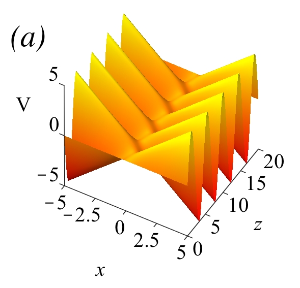
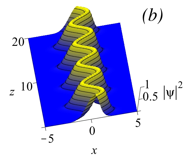
Figure 1: (Color online) (a) Linear coefficient (potential) and (b) modulated solution for the case 1. We have used $G=-1$, $\epsilon=-G$, and $\omega=\sqrt{2}$.

Case #2 - Next, we assume a nonlinear coefficient with an oscillatory amplitude. As an example, we use $\alpha=\left[1+\cos^{2}(\omega z)\right]/2$, $\beta=0$, and $\gamma$ with a specific choice such that $\delta_{3}=0$. In this case, one gets

$$\zeta=\left[0.5+0.5\cos^{2}(\omega z)\right]x$$ (20)

and

$$\tau=\left\{\left[11\cos\left(\omega z\right)+2\left(\cos\left(\omega z\right)\right)\right]\sin\left(\omega z\right)+19\omega z\right\}/32\omega.$$ (21)

Additionally, we have

$$V = \frac{1-5\cos^{2}\left(\omega z\right)+2\cos^{4}\left(\omega z\right)}{2\left[1+\cos^{2}\left(\omega z\right)\right]^{2}}\omega^{2}x^{2},$$ (22)

$$g = \frac{G}{4}\left[1+\cos^{2}\left(\omega z\right)\right]^{2}.$$ (23)

Also, the amplitude and phase of the solution are given by

$$\rho=\sqrt{1+\cos^{2}(\omega z)}/\sqrt{2},$$ (24)

and

$$\eta=\frac{\omega\cos\left(\omega z\right)\sin\left(\omega z\right)}{2[1+\cos^{2}\left(\omega z\right)]}x^{2}+\gamma,$$ (25)

respectively, where

$$\gamma=-\frac{1}{4}G[1+\cos^{2}(\omega z)]^{2}\ln[(1+\cos^{2}(\omega z))/2].$$ (26)

This allows us to find a new analytical solution for $\psi$. In Fig. 2 we show the profile of $|\psi|^{2}$ considering $G=-1$ (self-focusing nonlinearity), $\epsilon=-G$, and $\omega=1$. The potential assumes a flying-bird behavior that modulates the solution with a breathing pattern.

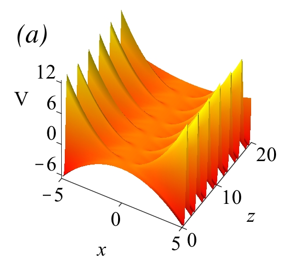
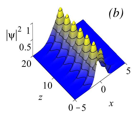
Figure 2: (Color online) (a) Linear coefficient (potential) and (b) modulated solution for the case 2. We have used $G=-1$ and $\omega=1$.

Case #3 - Another example can be introduced, after considering a linear potential with a combination of linear and quadratic terms in $x$, plus a periodic modulation in the $z$ coordinate. To this end, we can take

$$\alpha=\frac{1}{2}\left[1+\cos^{2}(\omega_{1}z)\right],$$ (27)

$$\beta=-2\sin(\omega_{2}z),$$ (28)

and $\gamma$ with a specific choice such that $\delta_{3}=0$. These choices allow us to write

$$\zeta=\frac{1}{2}\left[1+\cos^{2}(\omega_{1}z)\right]x-2\sin(\omega_{2}z),$$ (29)

$$\tau=\frac{1}{32\omega_{1}}\left\{\left[11\cos\left(\omega_{1}z\right)+2\cos^{3}\left(\omega_{1}z\right)\right]\sin\left(\omega_{1}z\right)+19\omega_{1}z\right\},$$ (30)

$$\delta_{1}=\frac{\omega_{1}^{2}\left[1-5\cos^{2}\left(\omega_{1}z\right)+2\cos^{4}\left(\omega_{1}z\right)\right]}{2\left[1+\cos^{2}\left(\omega_{1}z\right)\right]^{2}},$$ (31)

and

$$\delta_{2} = \frac{1}{\left[1+\cos^{2}\left(\omega_{1}z\right)\right]^{2}}\big{\{}2\omega_{2}\left[\omega_{2}+\omega_{2}\cos^{2}\left(\omega_{1}z\right)\right]\sin\left(\omega_{2}z\right)$$ (32)

$$- 8\omega_{2}\cos\left(\omega_{1}z\right)\omega_{1}\cos\left(\omega_{2}z\right)\sin\left(\omega_{1}z\right)\big{\}}.$$

Thus, we get the expected form $V=\delta_{1}x^{2}+\delta_{2}x$ and

$$g=\frac{G}{4}\left[1+\cos^{2}\left(\omega_{1}z\right)\right]^{2}.$$ (33)

Also, the amplitude and phase can be written in the form

$$\rho=\sqrt{\frac{1}{2}[1+\cos^{2}(\omega_{1}z)]},$$ (34)

and

$$\eta=\frac{\omega_{1}\cos\left(\omega_{1}z\right)\sin\left(\omega_{1}z\right)}{2[1+\cos^{2}\left(\omega_{1}z\right)]}x^{2}+\frac{2\omega_{2}\cos(\omega_{2}z)}{1+\cos^{2}(\omega_{1}z)}+\gamma,$$ (35)

respectively, where

$$\gamma = -\frac{1}{4}G[1+\cos^{2}(\omega_{1}z)]^{2}\ln[(1+\cos^{2}(\omega_{1}z))/2]$$ (36)

$$-\frac{4\omega_{2}^{2}\cos^{2}(\omega_{2}z)}{[1+\cos^{2}(\omega_{1}z)]^{2}}.$$

In Fig. 3 we depict the linear coefficient (potential) and the profile of the solution ($|\psi|^{2}$) , considering $G=-1$, $\epsilon=-G$, $\omega_{2}=2\omega_{1}=1$. This type of modulation makes the solution to oscillate in the $x$-direction, with a breathing profile. Also, solutions with quasiperiodic oscillation in $x$ and/or z can be found with an appropriate adjustment of the ratio $\omega_{1}/\omega_{2}$ as an irrational number.

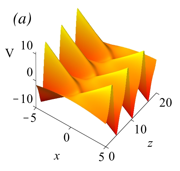
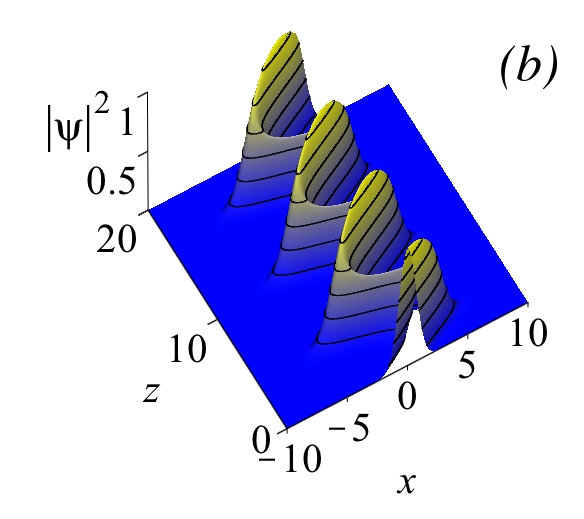
Figure 3: (Color online) (a) Linear coefficient (potential) and (b) modulated solution for the case 3. We have used $G=-1$, $\epsilon=-G$, and $\omega_{2}=2\omega_{1}=1$.

Stability analysis - The numerical method is based on the split-step Crank–Nicholson algorithm in which the evolution equation is splitted into several pieces (linear and nonlinear terms), which are integrated separately. A given trial input solution is propagated in time over small steps until a stable final solution is reached. To this end, we have used the step sizes $\mathrm{\Delta x}=0.04$ and $\mathrm{\Delta z=0.001}$ that provide a good accuracy in the final state MuruganandamCPC09 . To ensure the stability of the method we also checked the norm (power) and the energy of the solution defined by $P=\int_{-\infty}^{\infty}|\psi|^{2}\mathrm{dx}$ and

$$E=\int_{-\infty}^{\infty}\mathrm{dx}\left\{|\psi_{x}|^{2}+V|\psi|^{2}+g|\psi|^{2}\left(\log|\psi|^{2}-1\right)\right\},$$ (37)

respectively.

To study stability for the above cases we employ a random perturbation in the amplitude of the solution with the form

$$\psi=\psi_{0}[1+0.05\nu(x)],$$ (38)

where $\psi_{0}=\psi(x,0)$ is the analytical solution for the cases 1, 2, and 3, respectively, and $\nu\in[-0.5,0.5]$ is a random number with zero mean evaluated at each point of discretization grid in $x$-coordinate.

In Fig. 4 we show the numerical propagation of the input state given by Eq. (38) with $\psi(x,0)$ being the solution of the case 1 and the comparison between the input ($z=0$) and output ($z=1000$) states. Note in Fig. 4a that we have restricted the profile to the value $z=100$ due to the large number of oscillations when $z\gg 100$. In this case the norm is maintained in $P\simeq 1.76911$ with a standard deviation of $5\times 10^{-13}$ while the energy oscillates around $E\simeq 90\pm 14$.

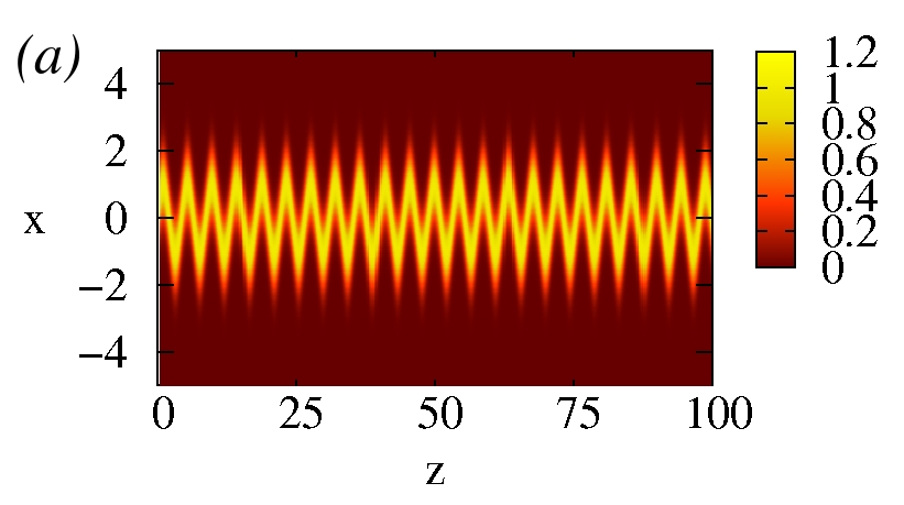
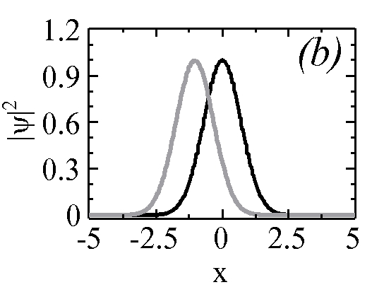
Figure 4: (Color online) Plot of the solution profile for the case 1 (a) in $x-z$ plane and (b) comparison between the input (black line) and output (grey line) solution in the $x$ dimension. The input state is taken at $z=0$ while the output state is in $z=1000$. Note in (b) that the input and output present the same profile with different peak positions due to the oscillations in the modulated snake-like solution. This implies the stability of the solution, at least until the observed $z$ value.

The numerical simulation of case 2 is displayed in Fig. 5. Here the breathing pattern is preserved even when the input state feels a small perturbation of the type shown in (38). Note that the Fig. 5b presents a difference in the amplitude of the input ($z=0$) and output ($z=1000$) states. This is due to the oscillatory pattern of the solution, but we stress that it is stable. We have obtained $P\simeq 1.76911$ with a standard deviation $\sim 10^{-13}$ and with a respective energy given approximately by $E\simeq 49\pm 12$ (with an oscillatory pattern).

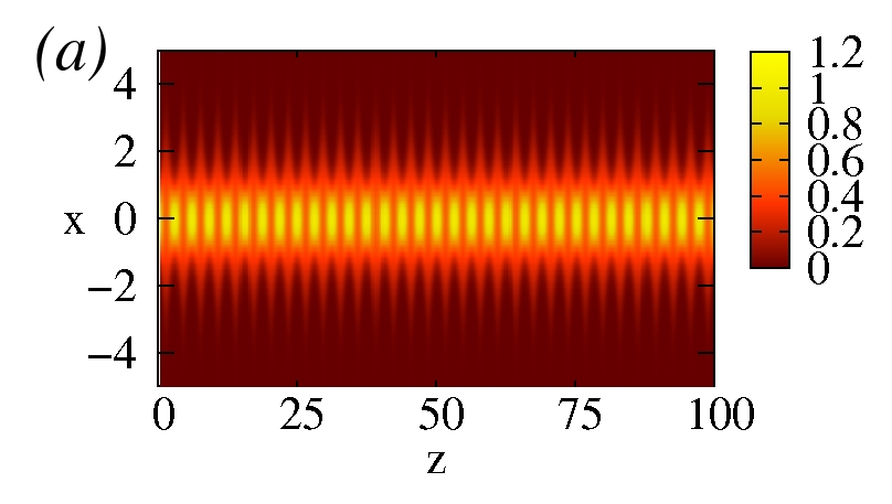
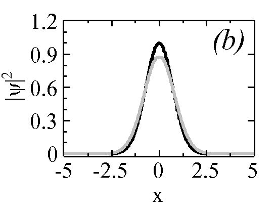
Figure 5: (Color online) Plot of the solution profile for the case 2 (a) in $x-z$ plane and (b) comparison between the input (black line) and output (grey line) solution in the $x$ dimension. The input state is taken at $z=0$ while the output state is at $z=1000$. Note in (b) that the input and output present different peak amplitudes due to the oscillations in the modulated solution.

In the last simulation we have checked the instability for the case 3. In Fig. 6 one can see the unstable behavior in the decay of the solution. The norm is given by $P\simeq 1.77096$ with a standard deviation $\sim 10^{-14}$ and the energy $E\simeq 186\pm 184$ (with a random pattern due to the instability).

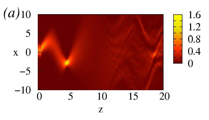
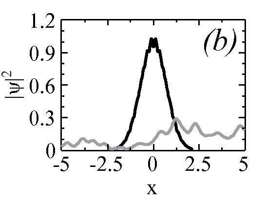
Figure 6: (Color online) Plot of the solution profile (a) in $x-z$ plane and (b) comparison between the input (black line) and output (grey line) solution in the $x$ dimension for the case 3. The input state is taken at $z=0$ while the output state is in $z=20$. Note that in this case the modulation induces an unstable behavior.

Conclusion - In this work we investigated the presence of analytical localized solutions to the LSE. We used similarity transformation to deal with inhomogeneous nonlinearity and potential. The inhomogeneities allowed us to modulate the pattern of the localized solution presenting a snake-like, breathing, and mixed oscillatory and breathing forms. The stability of the solutions was numerically checked and we have shown some stable solutions for the model investigated.

Acknowledgement - This work was supported by CAPES, CNPq, FAPESP and INCT-IQ (Instituto Nacional de Ciência e Tecnologia de Informação Quântica).

References

- (1) I. Bialynicki-Birula and J. Mycielski, Ann. Phys. 100, 62 (1976).
- (2) J. J. Bollinger, D. J. Heinzen, W. M. Itano, S. L. Gilbert, and D. J. Wineland, Proc. 12th Intl. Conf. on Atomic Physics, 461 (1990).
- (3) E. S. Hernandez and B. Remaud, Physica A 105, 130 (1980).
- (4) E. F. Hefter, Phys. Rev. A 32, 1201 (1985).
- (5) W. Krolikowski, D. Edmundson, and O. Bang, Phys. Rev. E 61, 3122 (2000).
- (6) H. Buljan, A. Siber, M. Soljacic, T. Schwartz, M. Segev, and D. N. Christodoulides, Phys. Rev. E 68, 036607 (2003).
- (7) S. De Martino and G. Lauro, Proceedings of the 12th Conference on WASCOM (2003).
- (8) S. De Martino, M. Falanga, C. Godano, and G. Lauro, EPL 63, 472 (2003).
- (9) T. Cazenave, Nonlinear Anal. 7, 1127 (1983).
- (10) T. Cazenave and A. Haraux, Ann. Fac. Sci. Univ. Toulouse 2, 21 (1980).
- (11) P. Guerrero, J. L. Lopez, J. Nieto, Nonlinear Anal. Real World Appl. 11, 79 (2010).
- (12) C. M. Khalique and A. Biswas, Int. J. Phys. Sci. 5, 280 (2010).
- (13) A. Biswas and D. Milović, Commun. Nonlin. Sci. Numerical Simulation 15, 3763 (2010).
- (14) A. Biswas, D. Milovic, and E. Zerrad, Opt. Photonic Lett. 03, 1 (2010).
- (15) A. Biswas, J. E. Watson Jr., C. Cleary, and D. Milovic, J. Infrared. Milli. Terahz. Waves 31, 1057 (2010).
- (16) Y. V. Kartashov, B. A. Malomed, and L. Torner, Rev. Mod. Phys. 83, 247 (2011).
- (17) J. Hukriede, D. Runde, and D. Kip, J. Phys. D 36, R1 (2003).
- (18) A. Biswas, C. Cleary, J. E. Watson Jr., and D. Milovic, Appl. Math. Comput. 217, 2891 (2010), and references therein.
- (19) J. Belmonte-Beitia, V. M. Perez-Garcia, V. Vekslerchik, and V. V. Konotop, Phys. Rev. Lett. 100, 164102 (2008); W. B. Cardoso, A. T. Avelar, and D. Bazeia, Nonlinear Anal.: Real World Appl. 11, 4269 (2010).
- (20) A. T. Avelar, D. Bazeia, and W. B. Cardoso, Phys. Rev. E 79, 025602(R) (2009); J. Belmonte-Beitia, and J. Cuevas, J. Phys. A: Math. Theor. 42, 165201 (2009).
- (21) J. Belmonte-Beitia and G. F. Calvo, Phys. Lett. A 373, 448 (2009).
- (22) W. B. Cardoso, A. T. Avelar, D. Bazeia, and M. S. Hussein, Phys. Lett. A 374, 2356 (2010); W. B. Cardoso, A. T. Avelar, and D. Bazeia, Phys. Rev. E 86, 027601 (2012).
- (23) W. B. Cardoso, A. T. Avelar, and D. Bazeia, Phys. Lett. A 374, 2640 (2010); A. T. Avelar, D. Bazeia, and W. B. Cardoso, Phys. Rev. E 82, 057601 (2010).
- (24) P. Muruganandam and S.K. Adhikari, Comp. Phys. Commun. 180, 1888 (2009).